Exponential Inflation with Gravity
Abstract
In this paper we shall consider an exponential inflationary model in the context of vacuum gravity. By using well-known reconstruction techniques, we shall investigate which gravity can realize the exponential inflation scenario at leading order in terms of the scalar curvature, and we shall calculate the slow-roll indices and the corresponding observational indices, in the context of slow-roll inflation. We also provide some general formulas of the slow-roll and the corresponding observational indices in terms of the -foldings number. In addition, for the calculation of the slow-roll and of the observational indices, we shall consider quite general formulas for which the assumption that all the slow-roll indices are much smaller than unity, is not necessary to hold true. Finally, we investigate the phenomenological viability of the model by comparing it with the latest Planck and BICEP2/Keck-Array observational data. As we demonstrate, the model is compatible with the current observational data for a wide range of the free parameters of the model.
pacs
04.50.Kd, 95.36.+x, 98.80.-k, 98.80.Cq,11.25.-wI Introduction
In modern theoretical cosmology there are two widely popular scenarios that describe in a consistent way the primordial evolution, the inflationary scenario [1, 2, 3] and bouncing cosmology [4, 5, 6, 7, 8, 9, 10, 11, 12, 13, 14]. Both scenarios are quite appealing, solving most of the shortcomings of the standard Big Bang cosmology, however there are still many theoretical challenges to address. In all cases, the theoretical models have to be eventually confronted with the current observational data coming from the Planck collaboration [15] and the BICEP2/Keck-Array [16]. Many models of modified gravity [4, 17, 18, 19] that describe inflation or bouncing cosmology, in various theoretical contexts, remain valid, since the confrontation with the observational data validates their consistency. For example, in the context of gravity and modified gravity in general, it is possible to provide a viable cosmological evolution for various inflationary scenarios [20, 21, 22, 23, 24, 25, 26, 27, 28, 29, 30, 31, 32, 33, 34, 36, 35], and also for bouncing cosmology [37, 38]. With regard to the inflationary scenario, the standard approach is to use a slow-rolling scalar field, and an epitome of a large class of viable scalar-tensor cosmological models is offered by the -attractor models [39, 40, 41], see also [42, 43], for an gravity description of the -attractors. As was demonstrated in Refs. [42, 43], gravity offers a fertile ground for the development of viable inflationary theories, even in the vacuum case. In this line of research, in this paper we shall consider an exponential model of inflation, in which the Hubble rate and the corresponding scale factor have the following form,
| (1) |
where and are real and positive constants. The model (1) is not so popular in the context of scalar-tensor inflationary theories, however it is very similar to the phantom Little Rip inflationary scenario [44, 45], in which case the Hubble rate is . We need to note that similar models of inflation were studied in Ref. [46]. Our first intention was to investigate if the phantom Little Rip inflationary scenario can be realized by gravity, and if the resulting inflationary cosmology is viable. It turns out that only when is negative, the gravity inflationary solution is viable. It is conceivable that the effective equation of state parameter is not phantom for the evolution (1), and actually it is . In the following sections we shall investigate which gravity can realize the cosmological evolution (1) at leading order in the large curvature limit, which corresponds to the inflationary era. By using the resulting gravity, we shall perform a detailed analysis of the inflationary dynamics, by assuming a slow-roll era evolution. Finally, we shall confront the resulting inflationary model with the current observational data and we shall analyze the parameter space in order to see the range of values of the parameters for which the viability can be achieved. As we demonstrate, the viability of the model comes for a wide range of parameters.
This paper is organized as follows: In section II we shall briefly present some essential features of vacuum gravity, which are necessary for the following sections. In section III we present the inflationary dynamics formalism and we express the slow-roll indices as functions of the -foldings number . We present in detail the formulas of the slow-roll indices and of the corresponding observational indices in terms of , and we consider the most general case for the approximate functional form of the observational indices. In section III, we employ a well-known reconstruction technique, in order to find the which realizes the exponential inflationary cosmology. In section IV we analyze in depth the parameter space and we investigate for which values of the free parameters, the exponential inflationary model in the context of gravity, can be viable. Finally, the conclusions follow in the end of this paper.
Before we proceed to the presentation of our results, we briefly present the geometric conventions we shall use in this paper. We shall consider a flat Friedmann-Robertson-Walker (FRW) spacetime, with the line element being,
| (2) |
and denotes the Universe’s scale factor. Moreover, we shall assume that the metric connection is a metric compatible affine connection, which is torsion-less and symmetric, the Levi-Civita connection.
II Basic Features of Gravity
In this section we shall briefly present some basic features of vacuum gravity, and for more details on this topic, the reader is referred to Refs. [4, 17, 18]. The 4-dimensional gravity gravitational action is equal to,
| (3) |
with being , being the determinant of the background metric, and also stands for the Planck mass. We shall employ the metric formalism, and upon variation of the action (3) with respect to the metric tensor , the gravitational equations of motion become,
| (4) |
which can be rewritten in the following way,
| (5) |
where stands for . By using the FRW metric of Eq. (2), the gravitational equations of motion take the following form,
| (6) | ||||
| (7) |
where and stand for and respectively, and also denotes the Hubble rate . In addition, the “dot” indicates differentiation with respect to the cosmic time, and in addition the Ricci scalar for the FRW metric (2) is equal to .
III Inflationary Dynamics of Gravity: Formalism
In this section we shall present the formalism of the gravity slow-roll inflationary dynamics. Details on the inflationary dynamics for gravity can be found in Refs. [20, 23, 24], see also Refs. [34, 35] for some recent literature on the subject. The slow-roll indices , for a general vacuum slow-roll gravity are,
| (8) |
with the function appearing in Eq. (20) being equal to,
| (9) |
Also, a very useful quantity related to the calculation of the scalar-to-tensor ratio, is , which is defined as follows,
| (10) |
The calculation of the observational indices for the model at hand may vary, depending on the values that the slow-roll indices take during the slow-roll era. In the general case, and if the slow-roll indices satisfy the spectral index of the primordial curvature perturbation is [20, 23, 24],
| (11) |
with the quantity being equal to,
| (12) |
In the particular case that , the spectral index is approximately equal to,
| (13) |
The scalar to tensor ration for a vacuum gravity is defined as follows [4],
| (14) |
where we defined in Eq. (10). After some algebra, in the case at hand, the scalar-to-tensor ratio reads,
| (15) |
In the particular case that , the scalar-to-tensor is greatly simplified, since and the above relation is simplified as follows,
| (16) |
In the rest of this section we shall investigate the behavior of the slow-roll indices during the slow-roll era, and in principle one can use the most appropriate definition of the observational indices we described above. However, regardless of the choice of the approximation one can use, with regard to the observational indices, namely Eqs. (11) and (13) for the spectral index, or Eqs. (14) and (15) for the scalar-to-tensor ratio, the viability of the theory is independent of the choice if the slow-roll indices satisfy the condition , . So in order to be as accurate as possible, we shall choose the formally more rigid approach, in which the spectral index is given by Eq. (11) and the scalar-to-tensor ratio is given by Eq. (15).
Before proceeding, let us further simplify the slow-roll indices appearing in Eq. (20), and after some algebra we obtain,
| (17) |
with and . For the purposes of our analysis, we shall express the above quantities in terms of the -foldings number , so by using the following differentiation rules,
| (18) |
| (19) |
the slow-roll indices become,
| (20) | ||||
Thus if the Hubble rate is known, and also the gravity which generates the evolution , then, the slow-roll indices and the corresponding observational indices can be found.
In order to proceed, let us express the exponential Hubble rate of Eq. (1), as a function of the -foldings number , so by solving the equation with respect to the cosmic time and by substituting the result in Eq. (1), the resulting expression for the Hubble rate is,
| (21) |
where is the integration constant appearing in the scale factor (1). Substituting the resulting Hubble rate of Eq. (21), in the slow-roll indices of Eq. (20), we obtain,
| (22) | ||||
Accordingly, the spectral index of the primordial curvature perturbations appearing in Eq. (11) reads,
| (23) |
where the function stands for,
| (24) |
Accordingly, the scalar-to-tensor ratio reads,
| (25) |
Thus what remains now to complete the study, is to find the gravity that generates the evolution (21). Then by expressing the Ricci scalar as a function of the -foldings number , we can find the the term appearing above, and the resulting expressions of the slow-roll indices and therefore also the observational indices can also be found. This is the subject of the next section.
IV Reconstruction of the Gravity Realizing the Exponential Inflationary Era
Let us now proceed to find the functional form of the gravity which realizes the evolution (21). To this end, we shall employ the reconstruction technique which was developed in Ref. [47]. The cosmological equation (6), can be cast in the following form,
| (26) |
By using the -foldings number , and also the differentiation rules of Eqs. (18) and (19), the Eq. (26) is written as follows,
| (27) | ||||
where the primes this time stand for and . We introduce the function , and by writing the differential equation (27) in terms of , we obtain,
| (28) |
with and . We can also express the Ricci scalar as a function of and it reads,
| (29) |
Hence, the gravity which realizes the Hubble rate can be found by solving the differential equation (28). Accordingly, we can find the quantity in terms of and by expressing as a function of by using Eq. (29), we can find the exact form of the slow-roll indices (22), and the observational indices can easily be obtained. In the case at hand, the function is,
| (30) |
and in effect, the algebraic equation (29) is equal to,
| (31) |
By solving the above with respect to the -foldings number , we obtain the following solution,
| (32) |
In order to obtain the gravity in a closed form, we shall focus on the large curvature limit, which corresponds to the slow-roll inflationary era, and thus, by using Eqs. (30) and (32), the differential equation appearing in Eq. (28), in the large limit becomes,
| (33) |
The differential equation (33) can be solved analytically, and the solution is,
| (34) |
where and are integration constants, and also the parameters and are defined as follows,
| (35) | ||||
The inflationary gravities of this type were also studied in Ref. [48]. Having the resulting form of the gravity at hand, enables us to calculate the spectral index of the primordial curvature perturbations and the scalar-to-tensor ratio, and we shall investigate the behavior of the observational indices in the next section.
V Inflationary Phenomenology and Confrontation with the Observational Data
Let us now turn our focus on the viability of the gravity model (34), which realizes the cosmological evolution (1), in the large curvature limit. So by using the functional form of the gravity (34) and also by substituting the Ricci scalar as a function of the -foldings number from Eq. (31), the observational indices (23) and (25) can be obtained in closed form. The parameter space is rich, and it consists of , , and , so the viability with the Planck and BICEP2/Keck-Array data can be obtained easily for a wide range of parameters. Before proceeding to the analysis of the parameter space, let us recall the observational constraints on the spectral index and the scalar-to-tensor ratio , coming from the Planck data [15], which are
| (36) |
while the BICEP2/Keck-Array data [16] further constrain the scalar-to-tensor ratio as follows,
| (37) |
at confidence level. Also, from Eq. (36) it is obvious that the spectral index can be considered as compatible with the Planck observations, when it takes values in the interval , so we shall take this into account in our analysis. Let us use some characteristic examples in order to see the viability of the model, so for , , and , the observational indices become,
| (38) |
and both are compatible with the Planck and BICEP2/Keck-Array data.
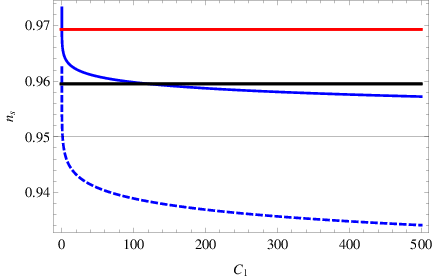
There is a large range of the parameters for which the viability of the model can be achieved, and in order to see this, in Fig. 1 we plotted the behavior of the spectral index as a function of for (blue thick curve) and for (dashed blue curve), and with the rest of the parameters being , . In the plots of Fig. 1, the upper red line corresponds to the value and the lower black curve corresponds to , which is the allowed range of . As it can be seen in Fig. 1, the viability is achieved for a large range of values of the parameter .
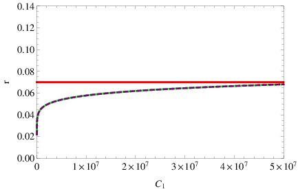
For the same range and values of the parameters, in Fig. 2 we plot the behavior of the scalar-to-tensor ratio, as a function of the parameter , with the green curve corresponding to and the dashed purple corresponding to . The upper red line corresponds the the BICEP2/Keck-Array upper limit . As it can be seen Fig. 2, the viability can be achieved for a large range of the parameter , as in the case of the spectral index. The same applies if other parameters are used, but we omit for brevity.
Before closing it is worth discussing the limiting values of the parameters and appearing in Eq. (35), as functions of . Particularly, in order for these parameters to be real, the parameter must be chosen in the following ranges,
| (39) |
Then it is easy to see how the resulting gravity behaves for the limiting values of the parameter . For example if is chosen to be very small, say , then the parameter is approximately equal to , while takes large values, that is , so the resulting gravity is,
| (40) |
so the subdominant term of the resulting gravity in this case resembles the Starobinsky model [62], however this is just the subdominant term. For , the gravity becomes approximately,
| (41) |
so the two terms have similar behavior. The viability of the resulting gravity can also be checked, and of course it is a different model from the Starobinsky model. Indeed, for , and , if the parameters and satisfy , the spectral index is equal to and the scalar-to-tensor ratio is . Now when is equal to , the gravity tends to,
| (42) |
and in this case if , , and , we get . Finally, for large values of , the parameter tends to while the parameter tends to . In this case the viability of the theory is questionable though, and can be achieved if the parameters and take abnormally large values. We omit this case since it is not so physically appealing. In conclusion, apart from the case that is extremely large, when the parameter satisfies the constraints (39), the resulting theory can be compatible with the observational data.
VI Conclusions
In this paper we studied an exponential inflationary evolution in the context of slow-roll vacuum gravity, and we analyzed the inflationary dynamics in some detail. Particularly, we expressed the slow-roll indices in terms of the -foldings number , and we calculated the spectral index of the primordial curvature perturbations and also the scalar-to-tensor ratio. For the calculation, the gravity which realizes the exponential inflationary scenario was needed, so by using well-know reconstruction techniques, we found the leading order functional form of the gravity, in the large curvature limit, which characterizes the inflationary era. As we demonstrated, the resulting inflationary theory is compatible with both the latest Planck and BICEP2/Keck-Array data, and the compatibility may be achieved for a large range of parameter values. Also we need to mention that exponential inflation theories of this type, may be the key element also for the construction of unified models of inflation with dark energy in various frames of gravity [49, 50].
An issue which we did not addressed is the graceful exit issue. In this theory, this may be achieved due to possible growing curvature perturbations, but this task is not easy to tackle in the context of the exponential inflationary theory. However, due to the fact that the Hubble rate is a quasi-de Sitter evolution, at leading order in the cosmic time, then the exit comes as an effect of growing curvature perturbations, as in Refs. [51]. Due to the complexity of this issue, and in order not to fall into inconsistencies, we hope to formally address this in a future work.
References
- [1] A. D. Linde, Lect. Notes Phys. 738 (2008) 1 doi:10.1007/978-3-540-74353-8_1 [arXiv:0705.0164 [hep-th]].
- [2] D. S. Gorbunov and V. A. Rubakov,“Introduction to the theory of the early universe: Cosmological perturbations and inflationary theory,” Hackensack, USA: World Scientific (2011) 489 p
- [3] D. H. Lyth and A. Riotto, Phys. Rept. 314 (1999) 1 doi:10.1016/S0370-1573(98)00128-8 [hep-ph/9807278].
- [4] S. Nojiri, S. D. Odintsov and V. K. Oikonomou, Phys. Rept. 692 (2017) 1 doi:10.1016/j.physrep.2017.06.001 [arXiv:1705.11098 [gr-qc]].
- [5] R. H. Brandenberger, arXiv:1206.4196 [astro-ph.CO].
- [6] R. Brandenberger and P. Peter, arXiv:1603.05834 [hep-th].
- [7] D. Battefeld and P. Peter, Phys. Rept. 571 (2015) 1 [arXiv:1406.2790 [astro-ph.CO]].
- [8] M. Novello and S. E. P. Bergliaffa, Phys. Rept. 463 (2008) 127 [arXiv:0802.1634 [astro-ph]].
- [9] Y. F. Cai, Sci. China Phys. Mech. Astron. 57 (2014) 1414 doi:10.1007/s11433-014-5512-3 [arXiv:1405.1369 [hep-th]].
- [10] J. de Haro and Y. F. Cai, Gen. Rel. Grav. 47 (2015) no.8, 95 [arXiv:1502.03230 [gr-qc]].
- [11] J. L. Lehners, Class. Quant. Grav. 28 (2011) 204004 [arXiv:1106.0172 [hep-th]].
- [12] J. L. Lehners, Phys. Rept. 465 (2008) 223 [arXiv:0806.1245 [astro-ph]].
- [13] Y. K. E. Cheung, C. Li and J. D. Vergados, arXiv:1611.04027 [astro-ph.CO].
- [14] Y. F. Cai, A. Marciano, D. G. Wang and E. Wilson-Ewing, Universe 3 (2016) no.1, 1 doi:10.3390/universe3010001 [arXiv:1610.00938 [astro-ph.CO]].
- [15] P. A. R. Ade et al. [Planck Collaboration], Astron. Astrophys. 594 (2016) A20 doi:10.1051/0004-6361/201525898 [arXiv:1502.02114 [astro-ph.CO]].
- [16] P. A. R. Ade et al. [BICEP2 and Keck Array Collaborations], Phys. Rev. Lett. 116 (2016) 031302 doi:10.1103/PhysRevLett.116.031302 [arXiv:1510.09217 [astro-ph.CO]].
- [17]
S. Nojiri, S.D. Odintsov,
Phys. Rept. 505, 59 (2011);
S. Nojiri, S.D. Odintsov, eConf C0602061, 06 (2006) [Int. J. Geom. Meth. Mod. Phys. 4, 115 (2007)]. - [18] S. Capozziello, M. De Laurentis, Phys. Rept. 509, 167 (2011);
- [19] A. de la Cruz-Dombriz and D. Saez-Gomez, Entropy 14 (2012) 1717 [arXiv:1207.2663 [gr-qc]].
- [20] H. Noh and J. c. Hwang, Phys. Lett. B 515 (2001) 231 [astro-ph/0107069].
- [21] J. D. Barrow and S. Cotsakis, Phys. Lett. B 214 (1988) 515. doi:10.1016/0370-2693(88)90110-4
- [22] A. R. Liddle, P. Parsons and J. D. Barrow, Phys. Rev. D 50 (1994) 7222 doi:10.1103/PhysRevD.50.7222 [astro-ph/9408015].
- [23] J. c. Hwang and H. r. Noh, Phys. Rev. D 65 (2002) 023512 doi:10.1103/PhysRevD.65.023512 [astro-ph/0102005].
- [24] J. c. Hwang and H. Noh, Phys. Lett. B 506 (2001) 13 doi:10.1016/S0370-2693(01)00404-X [astro-ph/0102423].
- [25] J. C. Hwang, Class. Quant. Grav. 7 (1990) 1613. doi:10.1088/0264-9381/7/9/013
- [26] S. Nojiri and S. D. Odintsov, Phys. Rev. D 68 (2003) 123512 doi:10.1103/PhysRevD.68.123512 [hep-th/0307288].
- [27] R. Ferraro and F. Fiorini, Phys. Rev. D 75 (2007) 084031 doi:10.1103/PhysRevD.75.084031 [gr-qc/0610067].
- [28] S. Nojiri and S. D. Odintsov, Phys. Rev. D 77 (2008) 026007 doi:10.1103/PhysRevD.77.026007 [arXiv:0710.1738 [hep-th]].
- [29] Q. G. Huang, JCAP 1402 (2014) 035 doi:10.1088/1475-7516/2014/02/035 [arXiv:1309.3514 [hep-th]].
- [30] J. c. Hwang, Phys. Rev. D 53 (1996) 762 doi:10.1103/PhysRevD.53.762 [gr-qc/9509044].
- [31] M. Artymowski and Z. Lalak, JCAP 1409 (2014) 036 doi:10.1088/1475-7516/2014/09/036 [arXiv:1405.7818 [hep-th]].
- [32] D. J. Brooker, S. D. Odintsov and R. P. Woodard, Nucl. Phys. B 911 (2016) 318 doi:10.1016/j.nuclphysb.2016.08.010 [arXiv:1606.05879 [gr-qc]].
- [33] L. Sebastiani and R. Myrzakulov, Int. J. Geom. Meth. Mod. Phys. 12 (2015) no.9, 1530003 doi:10.1142/S0219887815300032 [arXiv:1506.05330 [gr-qc]].
- [34] S. D. Odintsov and V. K. Oikonomou, Class. Quant. Grav. 33 (2016) no.12, 125029 doi:10.1088/0264-9381/33/12/125029 [arXiv:1602.03309 [gr-qc]].
- [35] S. D. Odintsov and V. K. Oikonomou, Phys. Rev. D 92 (2015) no.12, 124024 doi:10.1103/PhysRevD.92.124024 [arXiv:1510.04333 [gr-qc]].
- [36] V. K. Oikonomou, Int. J. Geom. Meth. Mod. Phys. 13 (2016) no.03, 1650033 doi:10.1142/S021988781650033X [arXiv:1512.04095 [gr-qc]].
- [37] S. D. Odintsov and V. K. Oikonomou, Phys. Rev. D 92 (2015) no.2, 024016 doi:10.1103/PhysRevD.92.024016 [arXiv:1504.06866 [gr-qc]].
- [38] S. D. Odintsov and V. K. Oikonomou, Int. J. Mod. Phys. D 26 (2017) no.08, 1750085 doi:10.1142/S0218271817500857 [arXiv:1512.04787 [gr-qc]].
- [39] R. Kallosh and A. Linde, JCAP 1307 (2013) 002 doi:10.1088/1475-7516/2013/07/002 [arXiv:1306.5220 [hep-th]].
- [40] S. Ferrara, R. Kallosh, A. Linde and M. Porrati, Phys. Rev. D 88 (2013) no.8, 085038 doi:10.1103/PhysRevD.88.085038 [arXiv:1307.7696 [hep-th]].
- [41] R. Kallosh, A. Linde and D. Roest, JHEP 1311 (2013) 198 doi:10.1007/JHEP11(2013)198 [arXiv:1311.0472 [hep-th]].
- [42] S. D. Odintsov and V. K. Oikonomou, Phys. Rev. D 94 (2016) no.12, 124026 doi:10.1103/PhysRevD.94.124026 [arXiv:1612.01126 [gr-qc]].
- [43] S. D. Odintsov and V. K. Oikonomou, arXiv:1611.00738 [gr-qc].
- [44] Z. G. Liu and Y. S. Piao, Phys. Lett. B 713 (2012) 53 doi:10.1016/j.physletb.2012.05.027 [arXiv:1203.4901 [gr-qc]].
- [45] P. H. Frampton, K. J. Ludwick, S. Nojiri, S. D. Odintsov and R. J. Scherrer, Phys. Lett. B 708 (2012) 204 doi:10.1016/j.physletb.2012.01.048 [arXiv:1108.0067 [hep-th]].
- [46] K. Bamba, S. Nojiri, S. D. Odintsov and D. Sáez-Gómez, Phys. Rev. D 90 (2014) 124061 doi:10.1103/PhysRevD.90.124061 [arXiv:1410.3993 [hep-th]].
- [47] S. Nojiri, S. D. Odintsov and D. Saez-Gomez, Phys. Lett. B 681 (2009) 74 doi:10.1016/j.physletb.2009.09.045 [arXiv:0908.1269 [hep-th]].
- [48] L. Sebastiani, G. Cognola, R. Myrzakulov, S. D. Odintsov and S. Zerbini, Phys. Rev. D 89 (2014) no.2, 023518 doi:10.1103/PhysRevD.89.023518 [arXiv:1311.0744 [gr-qc]].
- [49] S. Nojiri and S. D. Odintsov, Phys. Rev. D 68 (2003) 123512 doi:10.1103/PhysRevD.68.123512 [hep-th/0307288].
- [50] S. Nojiri and S. D. Odintsov, Phys. Lett. B 657 (2007) 238 doi:10.1016/j.physletb.2007.10.027 [arXiv:0707.1941 [hep-th]].
- [51] K. Bamba, R. Myrzakulov, S. D. Odintsov and L. Sebastiani, Phys. Rev. D 90 (2014) no.4, 043505 doi:10.1103/PhysRevD.90.043505 [arXiv:1403.6649 [hep-th]].
- [52] K. Bamba, A. N. Makarenko, A. N. Myagky and S. D. Odintsov, Phys. Lett. B 732 (2014) 349 doi:10.1016/j.physletb.2014.04.004 [arXiv:1403.3242 [hep-th]].
- [53] K. Bamba, S. D. Odintsov, L. Sebastiani and S. Zerbini, Eur. Phys. J. C 67 (2010) 295 doi:10.1140/epjc/s10052-010-1292-8 [arXiv:0911.4390 [hep-th]].
- [54] G. Cognola, E. Elizalde, S. Nojiri, S. D. Odintsov and S. Zerbini, Phys. Rev. D 73 (2006) 084007 doi:10.1103/PhysRevD.73.084007 [hep-th/0601008].
- [55] V. K. Oikonomou, Phys. Rev. D 92 (2015) no.12, 124027 doi:10.1103/PhysRevD.92.124027 [arXiv:1509.05827 [gr-qc]].
- [56] A. N. Makarenko, Int. J. Geom. Meth. Mod. Phys. 13 (2016) no.05, 1630006. doi:10.1142/S0219887816300063
- [57] Y. F. Cai, S. Capozziello, M. De Laurentis and E. N. Saridakis, Rept. Prog. Phys. 79 (2016) no.10, 106901 doi:10.1088/0034-4885/79/10/106901 [arXiv:1511.07586 [gr-qc]].
- [58] Y. F. Cai, S. H. Chen, J. B. Dent, S. Dutta and E. N. Saridakis, Class. Quant. Grav. 28 (2011) 215011 doi:10.1088/0264-9381/28/21/215011 [arXiv:1104.4349 [astro-ph.CO]].
- [59] S. Capozziello, M. De Laurentis and M. Francaviglia, Astropart. Phys. 29 (2008) 125 doi:10.1016/j.astropartphys.2007.12.001 [arXiv:0712.2980 [gr-qc]].
- [60] T. Clifton and J. D. Barrow, Class. Quant. Grav. 23 (2006) 2951 doi:10.1088/0264-9381/23/9/011 [gr-qc/0601118].
- [61] S. Chakraborty and S. SenGupta, Eur. Phys. J. C 76 (2016) no.10, 552 doi:10.1140/epjc/s10052-016-4394-0 [arXiv:1604.05301 [gr-qc]].
- [62] A. A. Starobinsky, Phys. Lett. B 91 (1980) 99. doi:10.1016/0370-2693(80)90670-X