Permutation glass

In statistical physics, spin glasses exist as archetypical models of disorder due both to their solubility and to the fact that they lend intuition to systems outside of physics which nonetheless exhibit properties common to many spin glasses. Soon after the first spin glass models were solved, physicists sought to apply the lessons of frustration, quenched disorder, and multiple equilibria to biological systems like neural networks [1, 2] and proteins [3]. But because biological systems integrate structure, function, and dynamics in ways not mirrored by any canonical model of physics, the utility of these spin glass models existed not in providing detailed predictions about biology but in supplying a quantitative framework in which to develop new ways of understanding and describing biological problems [4] .

In a previous work [5], we moved in the opposite direction: Rather than using our understanding of physics to develop new questions about biology, we used a biological question to motivate the inquiry into a physical system. Motivated by a computational examination of the protein design problem [6], we considered a statistical physics model of permutations in which the state space was isomorphic to the symmetric group. Significantly, the model’s motivation came, not from a physical system, but from a Monte Carlo study of a problem of biochemistry, and to establish intuition for it we considered lattice models where the energy costs were uniform across the system. But even with this simple assumption, the resulting permutation model had interesting thermal behavior because the non-factorizable nature of the state space conferred entropic disorder to a system which was nominally non-interacting. Thus the system exhibited thermal transitions among units which were coupled through state space even though they were not coupled in the Hamiltonian.

In this paper, we connect our study of the statistical physics of the symmetric group to disordered systems by considering the properties of a system with a state space of permutations and a quenched distribution of energy parameters. Given the unique nature of the state space and the solubility of the non-disordered analog, such a permutation glass [7] offers opportunities to explore the relationship between equilibria and disorder in simple exactly soluble physical systems.

In Sec. II of this paper, we discuss the original permutation model, provide schematic depictions of the systems to which it applies, and derive equations defining the thermal equilibrium of the permutation glass. In Sec. III we consider the permutation glass for various distributions of energy costs and derive transition temperatures for each case noting their overall consistency with the general result that $k_{B}T_{c}\leq\overline{\lambda}/\ln N$, where $\overline{\lambda}$ is the mean of the energy-cost distribution and $N$ is the number of components in the system. That is, the transition temperature of a permutation glass is always less than the transition temperature of the non-disordered system with energy cost given by $\overline{\lambda}$. In Sec. IV we compare the computed transition temperatures and a general expression for the order parameter of the permutation glass to results from simulations. In Sec. V we derive a distribution-independent result requiring that the “completely correct” state can only be a thermodynamic equilibrium of the system if $P_{\lambda<0}<1/N$ where $P_{\lambda<0}$ is the probability that an incorrectly-ordered component is energetically favored. In Sec. VI we use our derived results to define a glassy regime (which although not representing a distinct phase) cannot be found in the non-disordered system. In Sec. VII we conclude by discussing ways to extend this simple model of a permutation glass to more complicated models that could exhibit replica symmetry breaking, and we present an analogy between this system and a system of fermions.

In the statistical physics of permutations presented in [5], we considered a state space defined by a list of $N$ unique components $(\omega_{1},\omega_{2},\ldots,\omega_{N})$. Taking the states of the system to be the various $N!$ orderings of the components, and defining the zero-energy state as the state where the components are in the order $(\omega_{1},\omega_{2},\ldots,\omega_{N})$, we can postulate a simple Hamiltonian in which there is an energy cost $\lambda_{k}$ for each state where $\omega_{k}$ is not in the position given by its zero-energy ordering:

where $I_{A}=1$ if $A$ is true and $I_{A}$ = 0 otherwise, and $(\theta_{1},\theta_{2},\ldots,\theta_{N})\in\text{perm}(\omega_{1},\omega_{2},\ldots,\omega_{N})$. We term the state $\vec{\theta}=\vec{\omega}$ the “completely correct state,” and we say component $k$ of $\vec{\theta}$ is “incorrectly ordered” if it is not equal to $\omega_{k}$. The order parameter of our system is $\sum_{i=1}^{N}\langle I_{\theta_{i}\neq\omega_{i}}\rangle$, the average number of incorrectly ordered components of $\vec{\theta}$. We denote this average more succinctly as $\langle j\rangle$.

We can depict the various microstates of this system as a permutation graph, shown in Figure 1 for the case $N=15$. In each graph, whenever there is not a line connecting a lattice site $k$ to its vertical complement, the system gains a Boltzmann factor $e^{-\beta\lambda_{k}}$. The parameter $j$ is defined as the number of diagonal lines, and when $j=0$ we say the system is in the completely correct state.

Beyond a straightforward permutation interpretation of this model, there is an alternative (but formally equivalent) system which is defined by the Hamiltonian Eq.(1). Consider a collection of $2N$ subunits which only exist in $N$ labeled pairs where each pair consists of a black subunit and a white subunit, e.g., $(B_{1},W_{1}),(B_{2},W_{2}),\ldots(B_{2N},W_{2N})$. The various microstates of the system (an example of which is shown in Figure 2) are defined as the various ways the pairings could be arranged while ensuring that each pair has one black and one white subunit. If we associate an energy cost $\lambda_{k}$ with any pairing where $B_{k}$ is not paired with its associated $W_{k}$, then the statistical physics of the system would be identical to the statistical physics of the permutation model governed by Eq.(1). This amounts to the statistical physics of the “matching hat” problem [8].

In [5], we found that the statistical physics of such simple systems was quite interesting because even though their properties were governed by the Hamiltonian Eq.(1) in which distinct lattice sites did not interact, we could still have qualitative thermodynamically-driven changes in the properties of our system due to the nature of the state space. More quantitatively, for the system defined by the non-interacting Hamiltonian Eq.(1) with the global energy cost $\lambda_{i}=\lambda_{0}$ for all $i$, we can show (Appendix A) that the correlation between the incorrectness of two sites $i$ and $k$ (with $i\neq k$) is

for $\beta\lambda_{0}<\ln N$. Thus, as the temperature of our system decreases, the likelihood that component $i$ is incorrectly ordered given that $k$ is incorrectly ordered increases. Therefore, the sites are correlated in spite of the non-interacting Hamiltonian. For systems with correlated degrees of freedom, introducing disorder results in qualitative changes in the system’s thermal properties. So we can naturally wonder how disorder would affect a model in which the correlation arises at the level of the state space rather than the Hamiltonian.

We explore these ideas in a simple model of a permutation glass. We define a permutation glass as a statistical physics system with a state space consisting of various permutations of a list and with a Hamiltonian defined by a quenched distribution of parameter values. In a previous model, we set $\lambda_{i}=\lambda_{0}$ for analytic simplicity, but now we will maintain our distribution of $\lambda_{i}$ values.

By [5], the partition function for the system with Hamiltonian Eq.(1) is

Applying Laplace’s method to Eq.(3), we can define the approximate free energy ${\cal F}(s_{0})$ (modulo a thermodynamically irrelevant factor) according to

where

and where $s_{0}=s_{0}(\beta\lambda_{1},\cdots,\beta\lambda_{N})$ is defined by the critical point condition

We note that the second derivative of the argument of Eq.(5) yields

which is always greater than zero. Thus any critical point solution of Eq.(6) is also a stable thermal equilibrium.

Also, although Eq.(5) is in fact an approximation of the true free energy $\beta F=-\ln Z_{N}(\{\beta\lambda_{i}\})$, henceforth, we will work within our approximation and take Eq.(5) to be the free energy from which all thermodynamic quantities are computed. The validity of this approximation is coarsely constrained by parameter regimes over which $s_{0}$ yields a stable equilibrium for ${\cal F}$, and, by Eq.(7), this stability is itself only constrained by the physical relevance of the solutions to Eq.(6).

We can write Eq.(6) in a more physically transparent form. Noting that the average number of incorrect components $\langle j\rangle$ is the sum of $\langle I_{\theta_{i}\neq\omega_{i}}\rangle$ over all components, we have

Thus, we find

$\langle j\rangle=s_{0}-1$, and so Eq.(6) becomes

where $\langle j\rangle$ is the order parameter of our permutation system. Therefore, Eq.(9) defines the equilibrium of our system given the set of energy costs $\{\lambda_{k}\}$.

In order to find the equilibrium behavior governed by Eq.(9), it is useful to introduce a specific distribution of $\lambda_{\ell}$ values and convert Eq.(9) into an integral. For a sum over a general function $f(\lambda_{\ell})$, where the $\lambda_{\ell}$ are drawn from a normalized distribution $\rho_{0}(\lambda)$, we can write

Thus, with each $\lambda_{j}$ being drawn from the distribution $\rho_{0}(\lambda)$, Eq.(9) can be written as

This is not the typical way we start an analysis of glassy systems. Motivated by [9], the typical approach is to use the replica formalism to simplify the partition function and then use a stability analysis to check the validity of the simplification. Fortunately, as shown in Appendix B, the result Eq.(11) is consistent with the condition for the existence of the replica symmetric ansatz of the quenched free energy. More encouragingly, as our distribution $\rho_{0}(\lambda)$ becomes more centered around a single value $\lambda=\lambda_{1}$, we have $\rho_{0}(\lambda)\to\delta(\lambda-\lambda_{1})$, which leads to Eq.(11) reproducing the non-disordered behavior $\langle j\rangle\simeq N-e^{\beta\lambda_{1}}$ found in [5].

Eq.(11) does not appear any more soluble than Eq.(9), but we can use it to derive a general result characterizing one type of temperature-dependent behavior in this system: the thermal transition from $\langle j\rangle\neq 0$ to $\langle j\rangle=0$. Setting $\langle j\rangle=0$ in Eq.(11) for some $\beta_{c}$, we have

For a given distribution $\rho_{0}(\lambda)$, Eq.(12) can be computed and then inverted to find the temperature $k_{B}T_{c}=1/\beta_{c}$ at which the permutation glass achieves the $\langle j\rangle=0$ state. But even without detailed knowledge of the distribution, we can use Jensen’s inequality [10] to find an upper limit on this temperature. Given that $e^{x}$ is convex, and defining $\overline{f(\lambda)}\equiv\int d\lambda\rho_{0}(\lambda)f(\lambda)$ we have $\overline{e^{-\beta_{c}\lambda}}\geq e^{-\beta_{c}\overline{\lambda}}$, and thus by Eq.(12) we find

Eq.(13) states that the temperature at which the permutation glass achieves the completely correct $\langle j\rangle=0$ state is always less than the corresponding temperature predicted from the permutation system in which all interaction terms have the value $\lambda_{i}=\overline{\lambda}$. In essence, incorporating disorder into the interaction terms leads to a reduced tolerance for thermal disorder in achieving the $\langle j\rangle=0$ state. Moreover, Eq.(13) indicates that the $\langle j\rangle=0$ state is achievable only if the mean of the $\lambda$ distribution is positive.

We can derive an approximate expression for this transition temperature in the limit of small disorder. By the fact that the Fourier transform of $\rho_{0}(\lambda)$ is the exponential of the cumulant generating function [11], we find that Eq.(12) implies

where $\overline{\lambda^{n}}_{c}$ is the $n$th cumulant of the distribution $\rho_{0}(\lambda)$. Eq.(14) does not allow us to exactly solve for $\beta_{c}$ in terms of the cumulants, but it does allow us to solve for $\beta_{c}$ perturbatively assuming the series is dominated by the first and second cumulant. Noting the first cumulant is the mean $\overline{\lambda}$, the second cumulant is the variance $\sigma_{\lambda}^{2}$, and assuming $(\beta_{c}\sigma_{\lambda})^{2}\gg\beta_{c}^{k}\langle\lambda^{k}\rangle_{c}$ for $k>2$, we can approximately solve Eq.(14) to obtain

where we dropped the extraneous solution which yields $\beta_{c}\to\infty$ as $\sigma_{\lambda}\to 0$. Eq.(15) is a general result giving the temperature at which $\langle j\rangle=0$ transitions to $\langle j\rangle\neq 0$ (or vice-versa) for any distribution $\rho_{0}(\lambda)$, contingent on the assumption that the cumulants of order higher order than $2$ are subdominant. In spite of its limited validity, this result affords us some intuition into how small amounts of disorder affect the transition temperature of our system. If we take our distribution of energy costs to be highly peaked at $\overline{\lambda}$ with a small width $\sigma_{\lambda}\sqrt{2\ln N}\ll\overline{\lambda}$, we can expand Eq.(15) to find

where $T_{c}(0)\equiv T_{c}(\sigma_{\lambda}=0)=\overline{\lambda}/\ln N$ is the transition temperature for the non-disordered system. Consistent with Eq.(13), Eq.(16) shows that the effect of making our permutation system slightly glassy (i.e., imbuing it with nonzero $\sigma_{\lambda}$) is to lower the temperature at which the system transitions from $\langle j\rangle\neq 0$ to $\langle j\rangle=0$.

The qualitative explanation for this result is straightforward. Introducing disorder at the level of interactions effectively increases the entropy of our system, and the system then compensates for this additional entropy by making the thermal disorder limit for achieving the $\langle j\rangle=0$ state more stringent. In a sense, because of the interaction disorder, the free energy equilibrium of the system becomes less tolerant of thermal disorder. Thus, the transition temperature, a proxy for limiting thermal disorder, is reduced. A heuristic derivation employing this intuition and reproducing an order of magnitude estimate of Eq.(16) is provided in Appendix C.

To generalize this result, we cannot make direct use of the expansion Eq.(14): Since Eq.(15) and Eq.(16) do not apply when higher-order cumulants cannot be neglected, a perturbative analysis is not generally useful. Therefore when higher order cumulants are relevant, we have to calculate Eq.(11) analytically or numerically and then determine how the value and existence of $\beta_{c}$ depend on the properties of the chosen $\rho_{0}(\lambda)$. In the next section, we discuss how such properties affect $\beta_{c}$ by calculating the transition temperature for different energy-cost distributions.

We seek to affirm the theoretical transition temperatures of the previous section by comparing them to simulation results. Doing so requires us to simulate how $\langle j\rangle$ varies as a function of temperature when the $\{\lambda_{i}\}$ are drawn from the Gaussian, uniform, and symmetric Bernoulli distributions.

First, we derive a more general theoretical prediction to which we will compare the simulations. For the statistical physics of the non-disordered model where the Hamiltonian is ${\cal H}=\lambda_{0}\sum_{i}I_{\theta_{i}\neq\omega_{i}}$, we know the order parameter has the simple form

We would like to find analogous results for our permutation glasses defined by various distributions of energy costs. This would amount to computing Eq.(12) for a given distribution and inverting it to find $\langle j\rangle$ as a function of temperature and the parameters of the distribution. This procedure can be implemented exactly for the symmetric Bernoulli distribution, but there seems to be no analytic solution for the Gaussian or the uniform distribution. So, we will instead use a more general expression for $\langle j\rangle$ which allows us to reduce all the distribution-dependent order parameters to a common form.

Given the Hamiltonian Eq.(1) and that $\langle j\rangle$ is the sum of $\langle I_{\theta_{i}\neq\omega_{i}}\rangle$ across all components, we have

Then, using Eq.(3), yields the general result

where $Z_{N-1}(\{\beta\lambda_{i}\}_{i\neq k})$ is defined by Eq.(3) with the product taken over the $N-1$ elements of $\{\lambda_{i}\}$ not including $\lambda_{k}$. The utility of Eq.(34) is that it gives us the exact temperature dependence of the order parameter contingent on a particular distribution of energy costs. The caveat is that, rather than being a function of distribution parameters like means and variances, Eq.(34) requires us to draw the explicit set of $\{\lambda_{i}\}$ from the given distribution.

With Eq.(34), we have our theoretical prediction and can now discuss the simulation. The simulation was set up as follows: First, the vector $\vec{\omega}=(1,2,\ldots,N)$ was defined to be the completely correct permutation. This was the initial state in the simulation. Single-step state transitions were enacted by exchanging two randomly chosen elements of the current vector contingent on the Metropolis acceptance criterion, i.e., that $e^{-(E_{f}-E_{i})/T}<u$ where $E_{f}$ and $E_{i}$ were the final and initial state energies, respectively, $T$ was the temperature, and $u$ was a number drawn uniformly from $[0,1)$. The initial and final state energies were computed from Eq.(1) where the $\{\lambda_{i}\}$ were drawn from the given distribution defined by a mean $\lambda_{0}$ and variance $\sigma_{0}^{2}$. The simulation was run for $5\times 10^{4}$ steps of which the last $10^{3}$ steps were used to define the ensemble of states. From this ensemble of states, we computed $j$ (the number of elements in the state which did not match the corresponding element in $\vec{\omega}$) for each state and then averaged this value of $j$ across all states in the ensemble to find the simulation prediction of $\langle j\rangle$ at a specific temperature. We chose $30$ temperature values between $0.1$ and $1.3$. Finally, for a given distribution, the drawn set of $\{\lambda_{i}\}$ was used in Eq.(34) to obtain the corresponding theoretical prediction.

In Figures 4a, 4b, and 4c, we show simulation results for the parameter values $(N,\lambda_{0},\sigma_{0})=(50,1.0,0.35)$; respectively, these figures correspond to the Gaussian, uniform, and symmetric Bernoulli distribution of energy costs. As theory comparisons, for each distribution, we also plotted Eq.(34) for the same parameter values as in the simulation. We note that in all three cases, the theory curves well match the simulated results. As zero-disorder and high-disorder comparisons, we included theory curves of the order parameter for the standard deviation values $\sigma_{0}=0.0$ and $1.5$ with $N$ and $\lambda_{0}$ the same in all cases. From the differences in the curves among the plots, we see that at high disorder, the temperature behavior of Eq.(34) is greatly dependent on the distribution from which the $\{\lambda_{i}\}$ are drawn.

Finally, for Figure 4(a) and Figure 4(b), we computed the transition temperatures obtained from Eq.(19) and Eq.(23), respectively, and displayed the predictions as vertical dashed lines. Consistent with the simulation results, these lines correspond to the temperature values at which $\langle j\rangle$ transitions from zero to non-zero values or vice versa. Moreover, we note that, consistent with Figure 3, a disorder of $\sigma_{0}/\lambda_{0}=0.35$ allows the order parameter for the Gaussian and uniform distributions to reach $\langle j\rangle=0$ at sufficiently low temperatures, but, at this level of disorder, the order parameter for the symmetric Bernoulli distribution remains non-zero over its entire temperature range because its $k_{B}T_{c}$ does not exist.

The similarity between the theoretical and the simulation results is reassuring, but what still remains is the task of finding a unified interpretation for the constraints Eq.(20), Eq.(24), and Eq.(30). We turn to developing such an interpretation in the following section.

What is strange about the parameter conditions given by Eq.(20), Eq.(24), and Eq.(30) is their variety. Although each represents the conditions the mean and variance of the respective distribution must satisfy in order for the $\langle j\rangle=0$ state to be an equilibrium, they all have quite different scaling behaviors as functions of $N$. Perhaps most interestingly, the condition Eq.(24) becomes independent of $N$ in the $N\gg 1$ limit, thus suggesting that at large $N$ the amount of interaction disorder a system with a uniform distribution of energy costs can tolerate is independent of the number of microstates available to it.

However, underlying this variety in parameter conditions is a unity of the situations giving rise to them. Specifically, the conditions Eq.(20), Eq.(24), and Eq.(30) are the translations into distribution-parameter language of something which bears a common form when written as a probability. We can understand this by determining how the derived conditions place upper limits on the probability of obtaining an energy benefit, i.e., of drawing $\lambda<0$ from the distribution.

We begin with our previous constraint which must be satisfied in order for $\beta_{c}$ to exist:

Next, we define

which represents the probability that a $\lambda_{k}$ in Eq.(1) is less than zero (i.e., yields an energy benefit for an incorrectly ordered component rather than an energy cost). With the fact that $f(x)<e^{x}f(x)$ for $0<x$ and from Eq.(35), we can infer that in order for $\beta_{c}$ to exist (and, in turn, for the completely correct equilibrium $\langle j\rangle=0$ to be a physical state) we must have

Thus as $N\to\infty$, the probability of each lattice site having $\lambda<0$ must go to zero. Physically, we can interpret this result with the same intuition used to interpret Eq.(28). As the number of sites $N$ in our system increases, the number of potential incorrectly ordered microstates also increases, and thus to combat the entropic disorder from these microstates and to ensure the existence of the $\langle j\rangle=0$ equilibrium, the system must be ever more likely to have an energy cost (rather than an energy benefit) for incorrectly occupying a single site. Thus as $N$ increases, the system must become less tolerant of $\lambda<0$ values, and $P_{\lambda<0}$ goes to zero. Finally, the probability limit Eq.(37) is consistent with temperature limit Eq.(13) since both inequalities are derived from the same equilibrium condition.

Eq.(37) is a general result which must be true regardless of the distribution we choose, but what we find is that our previously derived mean-variance conditions are simply representations of Eq.(37) in the language of the parameters which define each specific distribution. To better understand how our mean-variance conditions Eq.(20), Eq.(24), and Eq.(30) are related to Eq.(37), we interpret them as placing upper limits on how much variance $\sigma_{0}^{2}$ the system can tolerate before the $\langle j\rangle=0$ state is no longer an equilibrium. Given that the $\langle j\rangle=0$ state is only achieved through the positive $\lambda$ domain of the distribution $\rho_{0}(\lambda)$, the upper limit on $\sigma_{0}$ must be tantamount to a lower limit on $\int^{\infty}_{0}d\lambda\,\rho_{0}(\lambda)$, or, equivalently an upper limit on $\int_{-\infty}^{0}d\lambda\,\rho_{0}(\lambda)$. Such an upper limit implies that if too much of the distribution is contained within the negative $\lambda$ domain, then the $\langle j\rangle=0$ state is not accessible. Thus interpreting Eq.(20), Eq.(24), and Eq.(30) as upper limits on the variances of their respective distributions, we can compute corresponding upper limits on the probability of obtaining a negative value of $\lambda$. For the relevant distributions we find (Appendix E)

The above expressions represent the maximum probability of having an energy benefit in the system and still being able to achieve the $\langle j\rangle=0$ state at a certain temperature. All of these results are unified by their inverse scaling with $N$ and, as shown in Figure 5, their consistency with the limit established by Eq.(37).

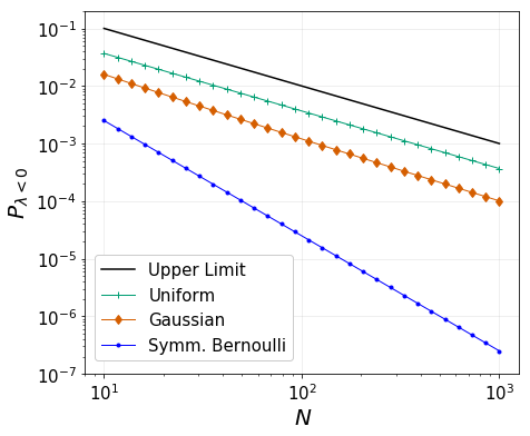
The results Eq.(38), Eq.(39), and Eq.(40) afford us a new interpretation of the results in Figure 3. We previously noted that the uniform distribution admitted the most amount of disorder before the $\langle j\rangle=0$ state was inaccessible and that the symmetric Bernoulli distribution admitted the least amount of disorder. From Figure 5 we see why: The uniform distribution allows the most amount of disorder because it admits the largest probability of energy benefits for incorrectly ordered components. By admitting a larger probability of energetically beneficial incorrect components, the distribution need not be tightly concentrated about the mean and can therefore have a higher standard deviation. Conversely, the symmetric Bernoulli distribution allows the least amount of disorder because it admits the smallest probability of energy benefits for incorrectly ordered components. The Gaussian distribution admits an intermediate value of disorder because its limiting probability exists between the limiting probabilities of the two other distributions.

Arguably, this explanation simply translates the old question into a new one: Why, conceptually, do the various distributions have the limiting probabilities shown in Figure 5? Their relative ordering could be understood by considering the $\lambda<0$ tails of each distribution. In order for the $\langle j\rangle=0$ state to be accessible, the distribution needs to be dominated by positive values of $\lambda$. We can roughly understand this by noting that in the non-disordered result Eq.(32), $\langle j\rangle=0$ is not accessible if $\lambda_{0}<0$. For the uniform distribution Eq.(21), it is possible to completely eliminate $\lambda<0$ values by simply increasing the ratio $\lambda_{0}/\sigma_{0}$ with $\sigma_{0}$ finite; thus for the uniform distribution, $\sigma_{0}$ can be finite and possibly large while the $\langle j\rangle=0$ state is still accessible. However, the long tail of the Gaussian Eq.(17) implies there will always be $\lambda<0$ values for non-zero $\sigma_{0}$. This is even more so for the symmetric Bernoulli distribution Eq.(25) since its probability density is not defined by an exponential fall off. Thus, in order to limit the $\lambda<0$ values, the Gaussian distribution needs to be less tolerant of large spreads than the uniform distribution, and the symmetric Bernoulli distribution must be even less tolerant than the Gaussian distribution. This relative tolerance of disorder leads to the sequence shown in Figure 5.

Lastly, noting that the results Eq.(38), Eq.(39), and Eq.(40) all scale at least as $\sim 1/N$ with corrections to the power of $N$ contingent on the distribution, we could guess there exists a stronger limit than Eq.(37) which any distribution must satisfy in order for $\beta_{c}$ to exist. Namely, in order for the $\langle j\rangle=0$ state to be achieved, we could conjecture that the probability of obtaining an energy benefit must satisfy, in the $N\gg 1$ limit,

where $\alpha(N)>0$ is dependent on the properties of the distribution.

In summary, the variety of results in the conditions placing limits on the distribution parameters is somewhat misleading because what is important is not the parameters themselves but the probabilities (specifically the probability of an energy benefit) they are associated with.

In the previous sections, we considered the conditions defining a permutations glass which allow for the existence of the $\langle j\rangle=0$ equilibrium. We pursued this analysis in analogy to the non-disordered system where the $\langle j\rangle=0$ state (found at temperatures below $\lambda_{0}/\ln N$) defined the only thermal transition in the system. From the discussion in Sec. V, we see that the permutation glass differs from the non-disordered system in that, for the permutation glass, it is possible to have a positive mean energy cost $\overline{\lambda}$ with the system still not transitioning to $\langle j\rangle=0$ at a physical temperature. The $\langle j\rangle=0$ macrostate is significant because it is the only macrostate for which the system has a single microstate and hence an entropy of zero. The number of microstates associated with a general $j$ is given by [5]

where $d_{j}$ is the number of derangements of a list with $j$ elements. We only find $\Omega_{N}=1$, when $j=0$ and thus if Eq.(35) cannot be satisfied at a physical temperature $k_{B}T_{c}$, the system always has a non-zero entropy.

Using Eq.(35), there are two results which are important in defining a glassy regime for this system. First, we recall the derived inequality

Eq.(43) requires that any temperature at which $\langle j\rangle=0$ is achieved to fall below ${\overline{\lambda}}/{\ln N}$ and, importantly, a necessary condition for such a temperature to exist is for $\overline{\lambda}>0$. For the case without quenched disorder (i.e., $\rho_{0}(\lambda)=\delta(\lambda-\overline{\lambda})$), the inequality in Eq.(43) becomes an equality, and the system always assumes the $\langle j\rangle=0$ macrostate when $k_{B}T$ falls below the stated value.

However, for quenched distributions an additional constraint must be satisfied. For the Gaussian, symmetric Bernoulli, and uniform two-parameter distributions analyzed in Sec III.1, the critical temperature takes on the general schematic form of $k_{B}T_{c}(\lambda_{0},\sigma_{0},N),$ where $\lambda_{0}$ and $\sigma_{0}$ are the mean and standard deviation of the distributions. For all of these analyzed distributions, we found that there was a minimum value of $\lambda_{0}/\sigma_{0}$ below which $k_{B}T_{c}(\lambda_{0},\sigma_{0},N)$ was no-longer physical. Namely, Eq.(35) has a real solution for $\beta_{c}$, if and only if

for some function $f(N)$ that depends on the properties of the distribution. In other words, even if $\overline{\lambda}>0$ and there are temperatures $k_{B}T$ that exist below $\overline{\lambda}/\ln N$, none of these temperatures would yield the $\langle j\rangle=0$ equilibrium unless Eq.(44) is satisfied as well. If Eq.(44) is violated, then even at zero-temperature we would have $\langle j\rangle\neq 0$ and, by Eq.(42), the entropy of the system would be non-zero. Therefore, when Eq.(44) is violated the system exhibits a zero-temperature residual entropy typical of glassy systems [13] and we can take a violation of Eq.(44) together with a positive $\overline{\lambda}$ to be definitive of the ”glassy regime” of the system.

These ideas become clearer with a concrete example and a figure. For a quenched distribution of energy-costs drawn from a Gaussian distribution, we found the critical temperature.

The phase diagram associated with this result is shown in Figure 6(a). The figure depicts the fact that, for $\lambda_{0}/\sigma_{0}<\sqrt{2\ln N}$, Eq.(45) becomes imaginary and the system enters the glassy regime and that although both the non-glassy and glassy regime have $\langle j\rangle\neq 0$ macrostates, unlike the non-glassy regime, the glassy regime never achieves $\langle j\rangle=0$ at a physical temperature.

We have already derived a more general condition for establishing the existence of the glassy regime. We found that a necessary, but not sufficient, condition for the $\langle j\rangle=0$ macrostate to exist is that $P_{\lambda<0}<1/N$. Therefore, a sufficient, but not necessary, condition for the system to exist in a glassy regime is for this inequality to be violated.

Looking beyond this result, we might expect the introduction of disorder into our permutation system to come with the multiple equilibria and ultrametricity of SK spin glasses [14]. However, for the class of permutation glasses considered here, this is not the case. We can see this by computing the Landau free energy for this disordered system. By Eq.(5), Eq.(10), and the substitution $s-1\to j$, we find

In Figure 6(b), we schematically plot this free energy, noting that it exhibits all of the functional forms of the free energy for the non-disordered case $\rho_{0}(\lambda)=\delta(\lambda-\lambda_{0})$. Mathematically, this arises due to its stability conditions: Because the free energy for the glassy system is always convex, it can have at most one minimum and, by the constraints of this system, this minimum must occur somewhere in the range of $0\leq j\leq N$. However, not all forms of this free energy are accessible for all parameter values in the system. In particular, for the glassy regime in which Eq.(35) has no solution, the free-energy curve with a global minimum at $\langle j\rangle=0$ cannot be achieved and the system has $\langle j\rangle\neq 0$ for all temperatures.

Thus, for the simple permutation glass considered in this paper, we say the system exists in the ”glassy regime” if and only if Eq.(35) does not admit a solution for $\beta_{c}$ even when the mean energy costs $\overline{\lambda}$ is greater than zero. This simplest version of a permutation glass does not exhibit the replica symmetry breaking and ultrametricity characteristic of SK glasses, but we argue for the labeling of a particular regime as ”glassy” due to its differing properties from the non-glassy regime: In the non-glassy regime, the disorder is not large enough to lead to thermal behavior different from that for the non-disordered system. However, in the glassy regime, the disorder is so large that at zero-temperature the system can exist in multiple microstates even if there is only a single free energy minima as a function of $j$.

Motivated by the importance of the orderings of amino acid sequences in the structure and function of proteins, a model was previously proposed to study the equilibrium thermodynamics of a system where particular permutations of an ordered list defined various energy states of the system. In that model, for simplicity and solubility, it was imposed that all lattice sites had the same energy cost for an incorrectly ordered component. However, more generally, it would have been useful to consider a system of permutations where the energy cost for each lattice site was drawn from a quenched distribution of energy costs.

We considered such permutation glasses here. The replica symmetric ansatz of such glasses yielded a result consistent with the thermodynamically stable state computed by applying Laplace’s method to the partition function. We found that this simplest permutation glass does not exhibit the replica symmetry breaking of spin glasses. However, it does exhibit a glassy regime–characterized by $\langle j\rangle\neq 0$ for all temperatures–if Eq.(35) cannot be satisfied even when $\overline{\lambda}>0$. In the non-glassy regime, the $\langle j\rangle=0$ state can be achieved but the transition temperature satisfies $k_{B}T_{c}\leq\overline{\lambda}/\ln N$, and thus the system is less tolerant of thermal disorder than is the non-disordered system in moving to the $\langle j\rangle=0$ state.

From this analysis we found that we must have $P_{\lambda<0}<1/N$ in order for $\langle j\rangle=0$ to be a possible macrostate, that is, in order for the completely correct ordering to be an achievable thermal equilibrium and for the system to be in the non-glassy regime, the probability of having an energy benefit for an incorrectly ordered component must be less than the inverse of the number of components in the system.

But having considered the permutation glass defined by the “non-interacting” Hamiltonian Eq.(1), a natural extension would be to consider a permutation glass with the typical spin glass-like Hamiltonian

where $\mu_{ij}$ is drawn from a distribution of interaction energies. Such a Hamiltonian associates an energy cost $\mu_{ij}$ with a permutation where both component $i$ and component $j$ are in an incorrect position. When the global analog of Eq.(47) was studied in [5], we found non-trivial regime behavior including multiple metastable states, multiple transition temperatures, and quadruple and triple points. Thus, considering the disordered behavior of a system with Hamiltonian Eq.(47), should yield some novel results (such as replica symmetry breaking) over the simpler phase behavior depicted in Figure 6(a).

Also, it is well known that spin glasses and other disordered systems often exhibit non-exponential relaxation behavior and memory effects [14], thus an interesting question would be whether such properties exist in kinetic permutation glasses. Answering such a question would likely require studying glasses defined by Eq.(47) rather than Eq.(1). In spin glass models, the glass transition temperature is important in defining the onset of such non-exponential relaxations. However, the analog of such a temperature does not seem to exist in the model defined by Eq.(1). Thus, before a kinetic analysis of permutation glasses can yield additional insights into the non-equilibrium properties of disordered systems, it would likely prove necessary to consider more complex glass models than the one considered in this paper.

Finally, we note that our free energy Eq.(46) is reminiscent of the thermodynamic potential of a familiar system in statistical mechanics. For a fermion system with a countably finite (but large) number of energy levels $N_{\text{lvl}}$ where each level is labeled $\varepsilon_{k}$ for some integer $k$, the grand canonical potential of the system is [15]

where $\mu$ is the chemical potential, $g(\varepsilon)$ is an energy density, and we used the heuristic Eq.(10) to replace the discrete sum with an integral. Comparing Eq.(46) for $j=\langle j\rangle$ to Eq.(48), we see that we can transform the former into the latter by making the substitutions $\beta F-1-\langle j\rangle\to\beta\Omega_{\text{Fermi}}$, $\rho_{0}(\lambda)\to g(\varepsilon)$, $N\to N_{\text{lvl.}}$, and $\langle j\rangle\to e^{\beta\mu}$.

With these substitutions, we find that for the fermion system the condition analogous to Eq.(11) is

We recall that for fermion gases in the grand canonical ensemble, the average number of fermions is given by

a result which is reproduced by Eq.(49) if we use the additional grand canonical ensemble constraint $\langle n_{\text{Fermi}}\rangle=e^{\beta\mu}$.

Given the transformation $\langle j\rangle\to e^{\beta\mu}$, we then see that Eq.(49) and Eq.(50) imply that in translating from a permutation glass to a fermion gas, we should interpret the order parameter $\langle j\rangle$ as the average number of fermions $\langle n_{\text{Fermi}}\rangle$. Therefore, the permutation glass inequalities $0\leq\langle j\rangle/N\leq 1$ correctly imply the fermion gas inequalities $0\leq\langle n_{\text{Fermi}}\rangle/N_{\text{lvl.}}\leq 1$. Thus, the canonical ensemble of a simple permutation glass seems to be dual to the grand canonical ensemble of a fermion system with a large number of energy levels and where the chemical potential is given by $\beta\mu=\ln\langle n_{\text{Fermi}}\rangle$.

Perhaps such a correspondence is not so surprising since permutations are central to the formalisms of both systems. Still, it is worth asking whether this duality can allow the understanding of one system to yield insights into the other.

The code for creating Figure 3, Figure 4, and Figure 5 can be found at: https://github.com/mowillia/permutation_code.

References

- [1] J. J. Hopfield, “Neural networks and physical systems with emergent collective computational abilities,” Proceedings of the national academy of sciences, vol. 79, no. 8, pp. 2554–2558, 1982.
- [2] J. J. Hopfield, “Neurons with graded response have collective computational properties like those of two-state neurons,” Proceedings of the national academy of sciences, vol. 81, no. 10, pp. 3088–3092, 1984.
- [3] J. D. Bryngelson and P. G. Wolynes, “Spin glasses and the statistical mechanics of protein folding,” Proceedings of the National Academy of Sciences, vol. 84, no. 21, pp. 7524–7528, 1987.
- [4] D. L. Stein, Spin glasses and biology, vol. 6. World scientific, 1992.
- [5] M. Williams, “Statistical physics of the symmetric group,” Physical Review E, vol. 95, no. 4, p. 042126, 2017.
- [6] E. I. Shakhnovich, “Protein design: a perspective from simple tractable models,” Folding and Design, vol. 3, no. 3, pp. R45–R58, 1998.
- [7] The phrase “permutation glass” was first used in [16] in reference to a self-assembly model with a single ground state and with degenerate low-energy microstates. In the current paper, the phrase refers to a system with a quenched disorder Hamiltonian and a state space consisting of not necessarily degenerate permutations.
- [8] J. K. Blitzstein and J. Hwang, Introduction to probability. CRC Press, 2014.
- [9] D. Sherrington and S. Kirkpatrick, “Solvable model of a spin-glass,” Physical review letters, vol. 35, no. 26, p. 1792, 1975.
- [10] D. Chandler, Introduction to modern statistical mechanics. Oxford University Press, 1987.
- [11] M. Kardar, Statistical physics of particles. Cambridge University Press, 2007.
- [12] E. W. Weisstein, “Lambert w-function,” Wolfram Mathworld, 2002.
- [13] S. V. Nemilov, “Zero-point entropy of glasses as physical reality,” Journal of Non-Crystalline Solids, vol. 355, no. 10-12, pp. 607–616, 2009.
- [14] K. Binder and A. P. Young, “Spin glasses: Experimental facts, theoretical concepts, and open questions,” Reviews of Modern physics, vol. 58, no. 4, p. 801, 1986.
- [15] L. D. Landau, E. Lifshitz, and L. Pitaevskii, Statistical Physics (Course of Theoretical Physics, Volume 5). Pergamon Oxford, 1980.
- [16] J. W. Collins, Self-assembly of colloidal spheres with specific interactions. Harvard University, 2014.