Development of -inverse model by using generalized polynomial chaos
Abstract
We present a -inverse model to estimate a smooth, non-negative source function from a limited number of observations for a two-dimensional linear source inversion problem. A standard least-square inverse model is formulated by using a set of Gaussian radial basis functions (GRBF) on a rectangular mesh system with a uniform grid space. Here, the choice of the mesh system is modeled as a random variable and the generalized polynomial chaos (gPC) expansion is used to represent the random mesh system. It is shown that the convolution of gPC and GRBF provides hierarchical basis functions for the linear source inverse model with the -refinement capability. We propose a mixed and regularization to exploit the hierarchical nature of the basis functions to find a sparse solution. The -inverse model has an advantage over the standard least-square inverse model when the number of data is limited. It is shown that the -inverse model provides a good estimate of the source function even when the number of unknown parameters () is much larger the number of data (), e.g., .
Keywords:
Inverse model, Advection-diffusion equation, Source estimation, Stochastic programming, Generalized polynomial chaos, Uncertainty quantification1 Introduction
Air pollution, generated by either anthropogenic or natural causes, poses a major public health threat. Not only long-term (Hoek et al., 2013), but also acute exposure (Phalen and Phalen, 2011) over a certain threshold can cause health problems. Due to its immense importance, there have been substantial development in the computational modeling of the transport of air-borne pollution over the past decade (Byun and Schere, 2006; El-Harbawl, 2013; Fast et al., 2006). However, prediction of air pollution by using these computational models requires extensive prior information on the distribution and magnitudes of pollution emission sources, which in most cases is incomplete or has high uncertainty (Thunis et al., 2016). Moreover, in many cases, it is of greater interest to identify the source of pollution when abnormally high pollution is observed in the air quality monitoring network to mitigate a possible public health hazard. This atmospheric inverse problem to find the pollution emission source using a set of measurements from a sensor network, has attracted significant attention in the atmospheric science community.
One of the fundamental building blocks of the inverse model is the atmospheric dispersion process, which is modeled by an advection-diffusion equation (Stockie, 2011). Deterministic approaches, adopted from the field of atmospheric data assimilation, have been used widely for the source inverse problem (Eckhardt et al., 2008; Issartel et al., 2007; Martinez-Camara et al., 2014; Pudykiewicz, 1998). In the deterministic approaches, typically a partial-differential-equation constrained optimization problem is solved to minimize a convex loss function, e.g., -distance between the computational model prediction and the observations. Since the optimization formulation for an inverse model usually leads to underdetermined or ill-conditioned system, much research effort is focused on regularizing the solution. Recently, inverse models exploiting Bayesian inference have become popular (Chow et al., 2008; Keats et al., 2007; Rajaona et al., 2015), due to the strength of the Bayesian methods in dealing with noisy and incomplete data. In Keats et al. (2007), the adjoint advection-diffusion operator is used to reduce the computational cost. Hwang et al. (2019) proposed an efficient Bayesian source inversion model to estimate the two-dimensional source function by exploiting the adjoint advection-diffusion operator. More general approaches to mitigate the high computational cost have been proposed by either accelerating the convergence of a Monte Carlo simulation (Marzouk et al., 2007), constructing surrogate models (Li and Marzouk, 2014), or developing a low-dimensional representation (Lieberman et al., 2010; Roosta-Khorasani et al., 2014).
Most of the previous inverse models consider either estimating the magnitudes of the source at each computational grid points by combining a large volume of heterogenous data (de Foy et al., 2015; Hwang et al., 2018; Issartel et al., 2007), or finding the locations and magnitudes of one or a few point sources from a limited number of data (Keats et al., 2007; Marzouk et al., 2007). In this paper, we propose an inverse model based on a regularized optimization formulation to estimate a smooth source function from a small number of observations. First, we follow the conventional approach of approximating a smooth function by a set of Gaussian radial basis functions centered at the collocation points of a rectangular mesh system. Obviously, the solution of the inverse models is strongly dependent on the choice of the mesh system. To relax the dependency on the mesh system, we introduce a random mesh system, in which the choice of the mesh system is modeled as a random variable. A stochastic inverse model is formulated on this random mesh system and the generalized Polynomial Chaos expansion (gPC) (Xiu, 2007) is employed to tackle the stochastic inverse problem. It is shown that the stochastic formulation leads to a -inverse model, in which the unknown smooth function is approximated by hierarchical basis functions. The -inverse model has an advantage over the standard least-square inverse model, particularly when the number of data is limited, due to its capability of -refinement (Karniadakis and Sherwin, 2005).
This paper is organized as follows. Section 2 describes a least-square formulation of the advection-diffusion problem by using an adjoint operator. In section 3, we reformulate the deterministic least-square problem as a stochastic problem by using gPC. In section 4, a mixed - and -regularization is introduced to exploit the hierarchical nature of the basis functions and an algorithm based on the alternating direction method of multipliers is presented to solve the optimization problem. The proposed inverse model is tested in section 5. Finally, the concluding remarks are given in section 6.
2 Least-square inverse model
2.1 Forward model
We consider the following advection-diffusion problem,
| (1) |
Here, is a rectangular domain , in which is the coordinate of the lower left corner of the domain and and are the lengths in the and directions, respectively, with the boundary , and denotes an outward normal vector on . The outflow and inflow boundaries are defined in terms of the fluid velocity as and . The fluid velocity is assumed to be given by a measurement or a computational fluid dynamics model. The advection-diffusion operator is defined as
| (2) |
in which is a symmetric second-order tensor of the diffusivity. We assume that the elements of and are smooth functions with uniformly bounded derivatives of all orders. The source strength is the unknown function, but assumed to be smooth. Furthermore, we consider a non-negative source, i.e., for every .
Contrary to the usual computational prediction problem, where equation (1) is solved for known to estimate at the sensor locations, the inverse model aims to estimate from the given observations at the observation time . Here, instead of estimating directly by solving an infinite dimensional optimization problem, is approximated by the sum of a set of basis functions to reduce the dimensionality of the problem. Let be a finite-dimensional approximation,
| (3) |
Here, is a set of basis functions, is the total number of the basis functions and denotes the coefficients. The problem of estimating a continuous surface is reduced to a problem of finding coefficients, . There are many possible choices for the basis functions as long as satisfies the non-negativity condition: . Here, a set of Gaussian radial basis functions (GRBF) located at the collocation points of a rectangular mesh is used as the basis functions;
| (4) |
in which is the distance between the neighboring collocation points, is the location of -th collocation point and is an parameter.
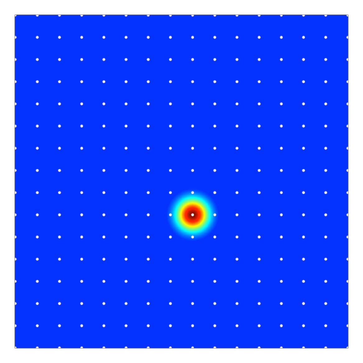
The rectangular mesh system is defined by a tensor product of two one-dimensional collocation sets,
| (5) |
Here, and denote the sets of collocation points in the - and -directions, respectively;
in which is the left and is the bottom end of the mesh system, and is the number of the collocation points in the -direction, . An example of and GRBF is shown in figure 1. Obviously, in the limit of , converges to the Dirac delta function and, hence, converges uniformly to . Using GRBF, the non-negativity condition can be satisfied by for .
Now, the advection-diffusion equation can be written as
| (6) |
Since is a linear operator, we can exploit the superposition of the solutions. Let be the solution for the -th GRBF;
Then, clearly,
Moreover, from the linearity of ,
| (7) |
Here, is the solution for with a unit strength, i.e., .
The computational model output is related to the observation by an inner product with respect to a sensor function () as
| (8) |
in which is the observation at the -th sensor, is the location of the -th sensor, is the time of the measurement, is the total number of the sensors, and is a Gaussian white noise representing the errors in the measurement as well as the computational model. The angle bracket denotes an inner product
The sensor function depends on the types of the sensor or the data used in the analysis. In this study, the sensor function is defined as
| (9) |
Here is a Heaviside function, which is zero for and one otherwise, and is an time-average window of the sensor.
By comparing (7) and (8), can be related to the measurement by
| (10) |
Here, and
| (11) |
The dispersion matrix relates to the observation . Since can be computed by solving exactly the same partial differential equation (2) for each GRBF (), the same numerical solver can be recycled.
The source strength can be obtained by finding from the following least-square minimization problem
| (12) |
in which is a regularization. Since we consider the case , is a rank-deficient matrix and a regularization is required to guarantee the uniqueness of the solution. We refer to (12) as a least-square (LS) inverse model.
2.2 Adjoint model
It is important to note that computing requires to solve the advection-diffusion equation for times, which makes it computationally impractical as becomes large. Moreover, as will be discussed in section 3, when the model uncertainty is considered, the total number of computation easily blows up to . To circumvent these difficulties, an adjoint model is employed in this study. Reducing the number of repetitive computations from the number of GRBFs, , to the number of observations, , an adjoint model is computationally more tractable (Keats et al., 2007).
Here, the adjoint model is briefly described. Define a conjugate field () as
| (13) |
Then, the adjoint operator is obtained from the Lagrangian duality relation;
| (14) |
which gives
| (15) |
for . The adjoint model (15) is solved backward in time from . For more details, see Pudykiewicz (1998).
Once the -th conjugate field is computed by solving (15) with appropriate boundary conditions (Hourdin et al., 2006), at the -th sensor is computed as
| (16) |
Repeating the process for conjugate fields, the observation vector is
| (17) |
in which
It is trivial to show that . The coefficients can be computed by solving the same least-square minimization problem (12).
3 Generalized polynomial chaos for model uncertainty
The Gaussian radial basis function, , distributes the source strength computed from (12) in the space centered on the collocation points of . Obviously, the solution of a LS inverse model depends on the choice of . For example, if a local peak of does not coincide with one of the collocation points, the LS inverse model will result in a poor accuracy. In general, there is no standard rule of choosing . In this study, we propose to represent the uncertainty in the choice of as a random variable.
Let be a random variable with a uniform distribution;
| (18) |
Here, and are real random variables defined over a probability space , in which is the sample space, is the -algebra, is the probability measure, and is an element of . Both and are defined over with the probability density functions, , , i.e. for , 2. Note that corresponds to a random translation of , which uniformly covers the entire computational domain. In the absence of prior information on the source location, a natural choice would be to give an equal probability to every possible .
On the random collocation system, , (17) becomes
| (19) |
in which
and
Here, we aim to model by the first moment of the stochastic system. Although it is possible to develop a model matching higher moments, it will lead to a complex non-convex optimization problem. Taking an expectation over , (19) becomes
| (20) |
Then, a least-square inverse model can be formulated as
| (21) |
in which
Note that, since we consider only the first moment, the non-negative condition is imposed only on the expectation of . Hereafter, the obvious dependence on is omitted in the expectation, i.e., .
Following Xiu (2007); Xiu and Karniadakis (2002), the generalized polynomial chaos (gPC) expansion is employed to approximate the stochastic functions;
| (22) | ||||
| (23) |
Here, is an orthonormal polynomial basis in a bivariate polynomial space () constructed by a tensor product of one-dimensional polynomial spaces
in which
As is a uniform random variable, the Legendre polynomial is chosen as the basis polynomial (Xiu and Karniadakis, 2002).


From the gPC approximation,
| (24) |
in which , , and denotes the total number of the basis functions excluding the mean (zero-th order) component, . Here,
| (25) |
And, the source function is
| (26) |
The gPC mode of GRBF, , is
| (27) |
The coefficients can be easily computed by using a numerical integration such as the Gaussian quadrature. For low order modes, can be even computed analytically. For example, the first mode of the expansion is
| (28) | ||||
Figure 2 shows the first four modes of . It is shown that constitutes spatial hierarchical basis functions to approximate . The advantage of using the hierarchical basis functions over increasing the number of GRBF () is discussed in section 4.
4 Regularized optimization formulation
Using the gPC expansion, the minimization problem (21) becomes,
| (29) |
In the minimization problem, the number of parameters to estimate is . Note that, if we use the forward simulation approach shown in section 2.1, even for and , the total number of numerical simulations to compute becomes . On the other hand, using the adjoint model, the total number of the numerical simulations remains as , which is and can be computed efficiently by evaluating the inner product with a numerical integration.
In (29), should satisfy the non-negativity constraint, for every . Because it is difficult to directly impose the non-negativity condition for every , we propose an indirect constraint based on the stochastic collocation approximation (Xiu and Hesthaven, 2005). In the stochastic collocation method, the stochastic functions are approximated by the Lagrange polynomials as
| (30) | ||||
| (31) |
Here, is the -th Lagrange polynomial, which is for the th collocation points in , . Again, is constructed by the tensor product of two one-dimensional Lagrange polynomials in and . The stochastic collocation method corresponds to a deterministic sampling and the coefficients are easily computed by the function evaluations at each collocation points in , i.e., and . Since GRBF is positivie, for all , the non-negativity condition implies for . In other words, in the stochastic collocation approach, it is sufficient to impose the non-negativity constraint only on the parameters, not on the field. The stochastic collocation coefficients, , are related to the modal gPC coefficients, , as
Then, the constraint on the smooth function surface for every can be approximated by the following linear constraint
| (32) |
Or,
| (33) |
in which is a block diagonal matrix for . In this study, we choose and (32) is evaluated at the Chebyshev node.
As an analogy to the finite element analysis (Karniadakis and Sherwin, 2005), either - or -type refinement can be used to increase the resolution of the proposed inverse model. Let be the number of GRBFs for a reference case, i.e., the number of collocation points of . In the -type refinement, the grid space is decreased as for , which makes the total number of unknown parameters . In the -type refinement, is fixed and the maximum order of is increased, which results in for . Because of this quadratic dependence, in both - and -type refinements, the number of unknown parameters can easily overwhelm the number of observations upon a refinement. For example, in the numerical experiments in section 5, the number of unknown parameters, i.e. the dimension of , is , while the number of data . As a result, the optimization formulation results in a highly ill-posed system, of which solution heavily relies on the choice of the regularization. To alleviate the difficulty, we develop a regularization strategy, which exploits the hierarchical nature of the GRBF-gPC coefficients, ,
As shown in (28), the zero-th gPC mode of GRBF, , represents the average source strength in centered at . Because , the non-negativity constraint implies that
| (34) |
At the same time, when the mean source strength, , is zero, the variation around the mean, represented by the higher-order gPC modes, should also be zero, i.e.,
| (35) |
Therefore, in the -type refinement, the number of unknown parameters can be effectively reduced by identifying non-zero elements in .
From these observations, we propose the following mixed - and -regularizations,
| (36) |
in which . The Least Absolute Shrinkage and Selection Operator (LASSO), or -regularization, is one of the most widely used regularization methods to find such a “sparse” solution for the so-called “large , small ” problem (large number of parameters and small number of data) (Tibshirani, 1996). As discussed above, for the -type refinement, applying LASSO only for is enough to guarantee a sparse solution. Hence, LASSO is applied only to the zeroth mode, , and the higher-order terms are regularized by the standard Tikhonov regularization.
From the non-negativity constraint, we know that . Then, the regularized optimization problem can be written as
| (37) | ||||
The first tuning parameter controls the sparsity in the solution, , and the second one prevents the overfitting by regularizing the total variation around the mean.
Furthermore, to consider the spatial smoothness of , the fused LASSO is used (Tibshirani et al., 2005). In the fused LASSO, -norm is imposed on the difference between a directly connected parameters. For example, in the -direction, the fused LASSO regularization is
| (38) |
in which is an index set for directly connected in the -direction, i.e.,
In other words, the fused LASSO is equivalent to imposing -penalty in the gradient of . We can define the difference matrix in the -direction, , similar to . Then, the regularization can be written as a mixed generalized LASSO (Tibshirani. and Taylor, 2011) and Tikhonov regularization,
| (39) |
in which
The coefficient determines the relative weight of the standard LASSO to the fused LASSO.
Finally, the optimization problem for the -type source reconstruction is
| (40) |
Note that the coupling between the modes shown in (35) is not explicitly imposed in the regularization. However, the sparsity in the modal domain is implicitly imposed through the linear constraint. This optimization problem is solved by using the Alternating Direction Method of Multipliers (ADMM). ADMM is one of the most widely used method for a large-scale optimization (Boyd et al., 2010).
Rewriting (40) as a constraint optimization problem,
| (41) |
where , , , and . Note that is padded with a null matrix , because the generalized LASSO, , is applied only to . The subscript indicates a projection onto a positive set , i.e., . The augmented Lagrangian form is
| (42) | ||||
in which is a constant. Then, the solution procedure for the minimization problem is as follows;
- 1.
Set initial conditions for and other variables.
Here, is an identity matrix of the dimension of , whose first elements are zero, which imposes the Tikhonov regularization on . Then,
- 2.
For , update by
- 3.
Next, update , i.e., and by
Here, is a vector of dimension , i.e., the number of GRBFs and the number of the quadrature points for the evaluation of the non-negativity condition. The operator takes only the upper elements of the vector for the generalized LASSO and subsets the lower elements of the vector for the non-negativity constraint.
- 4.
Finally, update ,
- 5.
Repeat steps 2 4, until the improvement
for a pre-specified tolerance level .
The Tikhonov regularization is imposed in Step 2. In Step 3, the fused LASSO is imposed on and the non-negativity constraint is imposed by a projection on the non-negative set in .
5 Numerical experiments
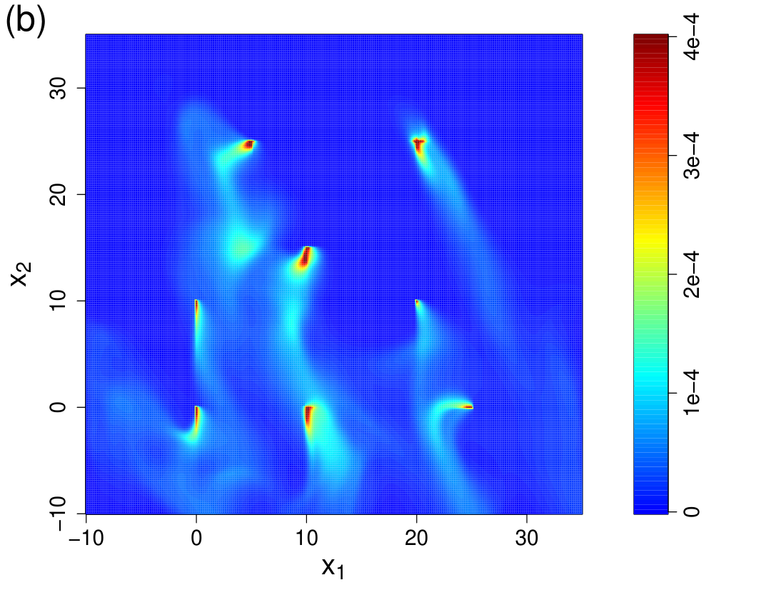
We use numerical simulations to study the behavior of the -inverse model and the results are compared with the standard least-square inverse models (12) with LASSO and fused-LASSO regularizations (Tibshirani et al., 2005; Tibshirani, 1996). The computational domain for this case study is . The adjoint equation (15) is numerically integrated for by using a third-order low-storage Runge-Kutta method and an upwind finite volume method. The computational grid and time step sizes are chosen as and .
Figure 3 (a) shows the computational domain as well as the locations of the sensors. The total number of observations is . The sensors are located at a rectangular mesh of which grid size is . The time averaging window of the sensor in equation (9) is and the time of observation is . The computational parameters are chosen similar to real operational air pollution measurement conditions. In an operational air pollution measurement, usually a high frequency sensor measurement is averaged over one to three hours to remove measurement noise.

A few adjoint functions are shown in figure 3 (b). To mimic the atmospheric dispersion process, the wind field is generated by a Fourier transform of a set of Ornstein-Uhlenbeck processes. The velocity in the -direction is
| (43) |
in which is the maximum number of the Fourier modes and is the wavenumber. The Fourier coefficients are computed by solving the following Langevin equation;
| (44) |
in which is a relaxation timescale, S is a scale parameter, and denotes the Wiener process . In this study, and are used (Pope, 2000). The velocity in the -direction is computed from the divergence-free condition;
| (45) |
In other words,
| (46) |
The mean components are also obtained by solving the same Langevin equation, but with . The diffusivity is computed by an isotropic Smagorinsky model, which is typically used in the atmospheric dynamics models (Byun and Schere, 2006):
Here, is the Kronecker delta, is the Smagorinsky coefficient, and the length scale . The velocity field is generated by one realization of the Ornstein-Uhlenbeck process and assumed to be known. Note that the velocity field is required only when computing .
5.1 Case study 1
5.1.1 Effects of refinement
Figure 4 (a) shows the true source surface, . The data is a snapshot of the concentration observation from the sensor network, shown in figure 4 (b). The goal is to estimate the source surface from the snapshot observation, of which size is .


Figure 5 shows the estimated source surface, , by the proposed -GRBF inverse model (gPC-LASSO) and the LS inverse models with fused LASSO, and LASSO regularizations. Hereafter, we use F-LASSO and LASSO to refer the LS inverse models with fused LASSO and LASSO regularizations, respectively. In gPC-LASSO, the grid space of the collocation set is and the scale parameter of GRBF, , is set to . The maximum order of the Legendre polynomial is in each direction. For F-LASSO and LASSO, and are used. The penalty parameter for regularization is set to for the all three models. For gPC-LASSO, the penalty parameter for regularization is . In gPC-LASSO and F-LASSO, is used. It is shown that gPC-LASSO provides a better approximation to the true source surface even with a lower resolution GRBF.
| 5 | 3 | 2 | 1 | |
|---|---|---|---|---|
| gPC-LASSO () | 0.034 | - | - | - |
| F-LASSO | 0.563 | 0.532 | 0.167 | 0.288 |
| LASSO | 0.576 | 0.505 | 0.449 | 1.713 |
For a quantitative comparison, we define a normalized error,
| (47) |
Table 1 shows for a range of . It is clearly shown that gPC-LASSO outperforms the other two standard LS models. By using -type refinement, i.e., reducing , of LASSO and F-LASSO decreases at first. Then, when is reduced from 2 to 1, starts to grow. This result demonstrates a shortcoming of the -type refinement of the LS inverse model, when only a limited number of observations is available. Refining the grid resolution of GRBF, the ratio of the number of unknown parameters to the number of observations of LASSO and F-LASSO increases from at to at . Hence, the solution of the LS inverse model becomes more strongly dependent on the regularization as the grid is refined. It is worthwhile to note that gPC-LASSO also has a large number of unknown parameters; . However, due to the hierarchical nature of the basis functions shown in (35), the number of unknown parameters to estimate is effectively reduced to , in which is the number of non-zero elements in . In this example, it is found that is 8.
In gPC-LASSO, although the grid space of is bigger than the size of the true emission source, the estimated source surface is very close to the true surface. Since gPC-LASSO uses a modal method to approximate the sub-grid scale variations, gPC-LASSO can provide a good estimate of the source surface even when the local maximum of is located in the middle of the GRBF collocation points. While F-LASSO correctly identifies the spatial pattern and the magnitude of the source (5 b), depends strongly on the choice of the collocation set . LASSO identifies the locations of large , but fails to provide a good approximation of the function surface. The ratio of maximum value of the source surface, , is 0.99 and 0.93 for gPC-LASSO () and F-LASSO (), respectively, while that of LASSO () is 1.46, as LASSO tries to fit the data with a fewer number of stronger sources.
Figure 6 shows the values of the modal coefficient . Among the total 1,764 parameters, there are only about 280 non-zero coefficients. It is shown that the magnitude of decreases as the order of polynomial increases, i.e. going right on the horizontal axis. The magnitudes of of the highest order polynomials are very small, indicating that the maximum order of Legendre polynomial used in this case study is enough to resolve .


In figure 7, gPC-LASSO is tested for two different collocation sets. From used in figure 5 (a), in figure 7 (a), is shifted in the -direction by and, in figure 7 (b), by in the -direction. As expected, it is shown that gPC-LASSO is not sensitive to the choice of the basis collocation set. The errors for the two new collocation sets are roughly the same, , which is very similar to the error of the reference case (figure 5 a), .


| 2 | 4 | 6 | 8 | 10 | |
|---|---|---|---|---|---|
| 0.437 | 0.231 | 0.145 | 0.077 | 0.069 |
Figure 8 shows from gPC-LASSO at a coarser grid resolution, . The same penalty parameters are used and , while the scale parameter is changed, . Figure 8 (a, b) shows the estimated source surfaces for two different maximum order of gPC expansion; and 8. For , gPC-LASSO under-resolves the source surface. When is increased to 8 (fig. 8 b), even with the large grid space, gPC-LASSO is able to approximate fairly well.
Table 2 shows as a function of . This corresponds to the -type refinement, where the grid resolution of GBRF is fixed and the maximum order of gPC expansion is increased to increase the fidelity of the estimation. Unlike the -type refinement of the LS inverse model in Table 1, monotonically decreases as increases in the range of tested. For a comparison, the ratio of the unknown parameters to the number of observations changes from at to at .
5.1.2 Effects of model parameters
In gPC-LASSO, there are two penalty parameters; and . As discussed in section 4, the penalty parameter controls the sparsity of the mean , while is related with the spectral decay of the variance, . To show the effects of these penalty parameters on the solution, is computed for a wide range of ad . In figure 9 (a), is shown as a function of for a fixed . The model resolutions of gPC-LASSO are and . In general, is not very sensitive to as long as is sufficiently small . For , seems to have a local minimum around , which then increases rapidly for a larger . It is worthwhile to note that decreasing does not have a significant effect on the solution, implying that the LASSO regularization does not play an important role in imposing sparsity in the solution. It is well known that, in a least-square regression problem, non-negativity constraint alone, without LASSO, is enough to recover sparsity (Buckstein et al., 2008; Slawski and Hein, 2011; Wang et al., 2011). In gPC-LASSO, although non-negativity constraint is not directly imposed on , the linear constraint () effectively imposes the non-negativity constraint on the mean components, , which explains why the generalized LASSO regularization for the mean component, , does not have a significant effect on the solution.
The effect of is shown in figure 9 (b). Again, is not sensitive to . However, when becomes larger than , the higher-order modes of are significantly suppressed, which results in the rapid increase of .
Another important parameter of gPC-LASSO is the lengthscale of the basis Gaussian envelope, . The scale parameter, , essentially controls the smoothness of the estimated source surface. Figure 10 shows the effects of on the square loss function,
together with the changes in . It is shown that has a local minimum around , while is almost constant up to , which starts to increase rapidly afterward. As is changed from 0.25 to 0.28, is increased by more than two orders of magnitude. For small , gPC-LASSO tries to approximate with sharp, peaked polynomials, resulting in a highly oscillatory surface. Hence, although gPC-LASSO is able to find a solution to faithfully fit , becomes large due to the high oscillation. On the other hand, for larger , the basis polynomials become too smooth to approximate , which makes both and grow. The optimal choice of seems to be related with both and the lengthscale of . It is challenging to decide the optimal a priori. However, figure 10 provides a guidance on how to select the scale parameter by performing a set of numerical tests, e.g., find the maximum which satisfies for a threshold level .
5.1.3 Noisy observations
To show the effects of the observation error on gPC-LASSO, the 36 observations are perturbed by an additive noise;
| (48) |
in which is a Gaussian random variable,
The parameter, , decides the signal-to-noise ratio. For a quantitative comparison, an ensemble error is computed from a Monte Carlo simulation with 200 samples;
Figure 11 shows the effects of the noise on the estimation error. Two resolutions are used for the comparison, and .
In figure 11 (a), the effects of the noise level are shown. The penalty parameters are fixed at , , and . Because we consider the problem of estimating the source surface from a small number of observations (), it is not surprising to see that the inverse model is sensitive to the noise. For , at , the ensemble error is about 0.22. while that of is 0.16. It is found that using a low resolution GRBF with a higher-order gPC mode makes gPC-LASSO less susceptible to the noise in the data.
The effect of LASSO for the noisy observation is shown in figure 11 (b). In this set of experiments, the noise level and the other penalty parameters are fixed at , , and . It is shown that, for , the -penalty does not play an important role. Similar to the noiseless case (figure 9), the ensemble error is insensitive to for smaller values of , and starts to grow when . On the other hand, for a finer resolution (), the -penalty makes gPC-LASSO more resistant to the noise. The ensemble error is shown to be a monotonically decreasing function of for .
5.2 Case study 2


| gPC-LASSO | F-LASSO | LASSO | |
| 0.04 | 0.13 | 0.14 |
In the second case study, the emission surface, , has a larger lengthscale than the grid space (figure 12 a), and the emission surface extends to the area not covered by the sensors. In figure 12 (b–d), from gPC-LASSO is compared with the solutions of F-LASSO and LASSO. The parameters of gPC-LASSO are chosen the same with the first case study, , , , and , except for the scaling parameter . For LASSO and F-LASSO, the model parameters are , , , and . It is again shown that gPC-LASSO provides a better approximation of . For a quantitative comparison, the normalized -error is listed in Table 3.
Figure 13 shows the behavior of with respect to the penalty parameters, and . Similar to the previous results (figure 9), it is shown that is not sensitive to and . Although the normalized error, , shows a local minimum around , the difference between the local minimum and at smaller is only 0.01.
Figure 14 (a) shows the effects of the -penalty parameter () on for the noisy observation, (48). The noise level is and is fixed, . The expectation and standard deviation of is computed by a Monte Carlo simulation with 200 samples. For the noisy observations, it is clearly shown that the -penalty has a significant impact on the accuracy of gPC-LASSO. When is very small, gPC-LASSO finds a solution which overfits the noisy data. In other words, gPC-LASSO results in a solution with a highly oscillatory surface to minimize the square loss function, , for the noisy observation. For a larger , the smoothness of the solution is recovered by the generalized LASSO regularization, which makes smaller. It is shown that, as increases, the standard deviation of is also reduced, implying that the generalized LASSO regularization also makes the estimation more robust to the noise.
The effects of the fused-LASSO parameter, , are shown in figure 14 (b). For this test, and are used. It is shown that using a higher value of results in a smaller error. However, the effects of on are not as significant as . There is about 10% reduction in the error as is increased from 0.1 to 0.8.
6 Summary
In this study, we present a -inverse model to estimate a source function from a limited number of data for an advection-diffusion problem. One of the standard methods of approximating a smooth source function, ), is to discretize the computational domain by a mesh system () and compute the coefficients, , of a basis function, such as GRBF. However, in such a mesh-based inverse model, the estimated function surface, , strongly depends on the choice of . To remove the dependence on the fixed mesh system, we formulate a stochastic least-square inverse model on a random mesh system, . The generalized polynomial chaos expansion (gPC) is employed to approximate the resulting stochastic functions; the source-receptor relation and the source strength .
By using gPC, a -inverse model is formulated, where is approximated by hierarchical polynomials. The -refinement approach has advantages over the conventional mesh-based method in that is not as strongly dependent on , and the spatial sparsity in can be more effectively recovered. The non-negativity constraint of , is replaced by a linear constraint, , by comparing the modal coefficients of gPC with the nodal coefficients of a stochastic collocation method. Finally, a mixed and regularization is proposed based on the hierarchical nature of the basis polynomials. An ADMM algorithm is presented to solve the regularized optimization problem.
The solution behavior of the proposed method (gPC-LASSO) is investigated for two case studies and the model error is compared with the mesh-based least square inverse methods with two most widely used regularization methods, LASSO and fused LASSO. It is confirmed that gPC-LASSO is not sensitive to the choice of and provides a very good approximation to the source surface even when the number of unknown parameters is more than 40 times larger than the number of data. It is shown that gPC-LASSO outperforms both LASSO and fused LASSO. For the noise-free data, the regularization does not play an important role for gPC-LASSO because the non-negativity constraint alone is enough to explore the sparsity in the solution. However, when noisy is added to the observations, the regularization provides a more robust approximation by enforcing the smoothness in the solution.
In summary, we show that a -inverse model can be developed by converting the deterministic problem to a stochastic problem and the -refinement capability has an advantage in exploring the sparsity structure in the data. We expect that the proposed framework can be applied to a broader class of problems, such as a general data-driven function estimation problem for a smooth, non-negative function. It should be noted that we limited our focus on a two-dimensional source inverse model for a steady emission in this study. It is a subject of the follow-up study how to generalize the framework to consider a much more complex problem of nonlinear inversion or estimation of unsteady emission sources.
References
- Boyd et al. (2010) Boyd S, Parikh N, Chu E, Peleato B, Eckstein J. Distributed optimization and statistical learning via the alternating direction method of multipliers. Foundations and Trends in Machine Learning 2010;3(1):1–122.
- Buckstein et al. (2008) Buckstein A, Elad M, Zibulevsky M. On the uniqueness of nonnegative sparse solutions to underdetermined systems of equations. IEEE Trans Inf Theory 2008;54:4813–20.
- Byun and Schere (2006) Byun D, Schere KL. Review of the governing equations, computational algorithms, and other components of the models-3 community multiscale air quality (CMAQ) modeling system. Appl Mech Rev 2006;59:51–77.
- Chow et al. (2008) Chow FK, Kosovic B, Chan S. Source inversion for contaminant plume dispersion in urban environments using building-resolving simulations. J Appl Meteor Climatol 2008;47:1553–72.
- de Foy et al. (2015) de Foy B, Cui YY, Schauer JJ, Janssen M, Turner JR, Wiedinmyer C. Estimating sources of elemental and organic carbon and their temporal emission patterns using a least square inverse model and hourly measurements from the St. Louis-Midwest supersite. Atmos Chem Phys 2015;15:2405–27.
- Eckhardt et al. (2008) Eckhardt S, Prata AJ, Seibert P, Stebel K, Stohl A. Estimation of the vertical profile of sulfur dioxide injection into the atmosphere by a volcanic eruption using satellite column measurements and inverse transport modeling. Atmos Chem Phys 2008;8:3881–97.
- El-Harbawl (2013) El-Harbawl M. Air quality modelling, simulation, and computational methods: a review. Environ Reviews 2013;21:149–79.
- Fast et al. (2006) Fast J, Jr. WIG, Easter RC, Zaveri RA, Barnard JC, E. G C, Grell GA. Evolution of ozone, particulates, and aerosol direct forcing in an urban area using a new fully-coupled meteorology, chemistry, and aerosol model. J Geophys Res 2006;111:D21305.
- Hoek et al. (2013) Hoek G, Krishnan RM, Beelen R, Peters A, Ostro B, Brunekreef B, Kaufman JD. Long-term air pollution exposure and cardio-respiratory mortality: a review. Environ Health 2013;12:43.
- Hourdin et al. (2006) Hourdin F, Talagrand O, Idelkadi A. Eulerian backtracking of atmospheric tracers. II: Numerical aspects. Q J Roy Meteor Soc 2006;132(615):585–603.
- Hwang et al. (2018) Hwang Y, Barut E, Yeo K. Statistical-physical estimation of pollution emission. Statistica Sinica 2018;28.
- Hwang et al. (2019) Hwang Y, Kim HJ, Chang W, Yeo K, Kim Y. Bayesian pollution source identification via an inverse physics model. Comput Stat Data Anal 2019;in press.
- Issartel et al. (2007) Issartel JP, Sharan M, Modani M. An inversion technique to retrieve the source of a tracer with an application to synthetic satellite measurements. Proc R Soc A 2007;463:2863.
- Karniadakis and Sherwin (2005) Karniadakis GE, Sherwin SJ. Spectral/ Element Methods for Computational Fluid Dynamics. Oxford University Press, New York, 2005.
- Keats et al. (2007) Keats A, Yee E, Lien FS. Bayesian inference for source determination with applications to a complex urban environment. Atmos Environ 2007;41(3):465 –79.
- Li and Marzouk (2014) Li J, Marzouk YM. Adaptive construction of surrogates for the Bayesian solution of inverse problems. SIAM J Sci Comput 2014;36:A1163 –86.
- Lieberman et al. (2010) Lieberman C, Willcox K, Ghattas O. Parameter and state model reduction for large-scale statistical inverse problems. SIAM J Sci Comput 2010;32:2523–42.
- Martinez-Camara et al. (2014) Martinez-Camara M, Bejar Haro B, Stohl A, Vetterli M. A robust method for inverse transport modeling of atmospheric emissions using blind outlier detection. Geosci Model Dev 2014;7:2303–11.
- Marzouk et al. (2007) Marzouk YM, Najm HN, Rahn LA. Stochastic spectral methods for efficient Bayesian solution of inverse problems. J Comput Phys 2007;224:560–86.
- Phalen and Phalen (2011) Phalen RF, Phalen RN. Introduction to Air Pollution Science. Jones & Bartlett Learning, 2011.
- Pope (2000) Pope SB. Turbulent flows. Cambridge University Press, 2000.
- Pudykiewicz (1998) Pudykiewicz J. Application of adjoint tracer transport equations for evaluating source parameters. Atmos Environ 1998;32:3039–50.
- Rajaona et al. (2015) Rajaona H, Septier F, Armand P, Delignon Y, Olry C, Albergel A, Moussafir J. An adaptive bayesian inference algorithm to estimate the parameters of a hazardous atmospheric release. Atmos Environ 2015;122:748 –62.
- Roosta-Khorasani et al. (2014) Roosta-Khorasani F, van den Doel K, Ascher U. Stochastic algorithms for inverse problems involving PDEs and many measurements. SIAM J Sci Comput 2014;36:3 – 22.
- Slawski and Hein (2011) Slawski M, Hein M. Sparse recovery by thresholded non-negative least squares. In: NIPS 2011. 2011. p. 1926–34.
- Stockie (2011) Stockie JM. The mathematics of atmospheric dispersion modeling. SIAM Review 2011;53:349–72.
- Thunis et al. (2016) Thunis P, Miranda A, Baldasano J, Blond N, Douros J, Graff A, Janssen S, Juda-Rezler K, Karvosenoja N, Maffeis G, Martilli A, Rasoloharimahefa M, Real E, Viaene P, Volta M, White L. Overview of current regional and local scale air quality modelling practices: Assessment and planning tools in the EU. Environ Sci Policy 2016;65:13–21.
- Tibshirani (1996) Tibshirani R. Regression shrinkage and selection via the lasso. J Royal Statist Soc B 1996;58:267–88.
- Tibshirani et al. (2005) Tibshirani R, Saunders M, Rosset S, Zhu J, Knight K. Sparsity and smoothness via the fused lasso. J Royal Statist Soc B 2005;67(1):91–108.
- Tibshirani. and Taylor (2011) Tibshirani. RJ, Taylor J. The solution path of the generalized lasso. Ann Statist 2011;39(3):1335–71.
- Wang et al. (2011) Wang M, Xu W, Tang A. A unique nonnegative solution to an underdetermined system: from vectors to matrices. IEEE Trans Signal Process 2011;59:1007–16.
- Xiu (2007) Xiu D. Efficient collocational approach for parametric uncertainty analysis. Commun Comput Phys 2007;2:293–309.
- Xiu and Hesthaven (2005) Xiu D, Hesthaven JS. High-order collocation methods for differential equations with random inputs. SIAM J Sci Comput 2005;27:1118–39.
- Xiu and Karniadakis (2002) Xiu D, Karniadakis G. The Wiener-Askey polynomial chaos for stochastic differential equations. SIAM J Sci Comput 2002;24:619–44.