Symmetry, chaos and temperature in the one-dimensional lattice theory
Abstract
The symmetries of the minimal theory on the lattice are systematically analyzed. We find that symmetry can restrict trajectories to subspaces, while their motions are still chaotic. The chaotic dynamics of autonomous Hamiltonian systems are discussed, in relation to the thermodynamic laws. Possibilities of configurations with non-equal ideal gas temperatures in the steady state, in Hamiltonian systems, are investigated, and examples of small systems in which the ideal gas temperatures are different within the system are found. The pairing of local (finite-time) Lyapunov exponents are analyzed, and their dependence on various factors, such as the energy of the system, the characteristics of the initial conditions are studied, and discussed. We find that for the theory, higher energies lead to faster pairing times. We also find that symmetries can impede the pairing of local Lyapunov exponents, and the convergence of Lyapunov exponents.
I Introduction
Chaotic properties of Hamiltonian systems have been studied for some time, and a general picture of the dynamics seems to be emerging[2, 3]. Yet interesting questions from the physics point of view still remain. Some of these issues were raised in [4], which we address in this work. In a dynamical system with chaos, trajectories with different initial conditions diverge exponentially from each other in the phase space, so that it may seem difficult to control its region of motion. The domain within the phase space in which it travels in can be restricted for energetic reasons. The possibilities of the symmetries of the dynamical system limiting the allowed region of motion is investigated in this work. The symmetries of the minimal theory, which has no additional symmetries, is investigated systematically. It is found that symmetries can indeed restrict the trajectories of the dynamical system in the phase space to its lower dimensional subspace. This property is not restricted to small systems.
Contrast to regular motions, where the trajectories are confined to specific regions in the phase space, chaotic trajectories can travel freely within the constant energy subspace of the phase space. Therefore, chaotic motions are sometimes used for simulations of finite temperature systems. Indeed, apart from quantum effects, this should be able to describe a real physics system, given enough degrees of freedom. The temperature for such systems can be well defined, but it is unclear whether the properties of finite temperature systems are reproduced, in general. In this work, Hamiltonian systems are used to simulate the dynamics of finite temperature lattice systems, and the physical properties of the system is investigated from the point of view of the basic thermodynamic laws. It is found that the basic law that the temperature within a thermally equilibriated system is uniform, can be violated in certain cases. We demonstrate this with a few examples, and analyze why it can occur.
Chaoticity of a system can be analyzed quantitatively through its Lyapunov exponents. For this purpose, the time averaged Lyapunov exponents over trajectories are usually studied. For autonomous Hamiltonian systems, these exponents are composed of pairs, which each sum to zero. One can also study the local, or the finite time, Lyapunov exponents, which have not been averaged over time. Interestingly, the local Lyapunov exponents are in general not paired, even in autonomous Hamiltonian systems, but seem to become paired after some time. This pairing property is studied in this work for the theory. It is found that the pairing time is faster at higher energies, and that the symmetries of the system can affect the pairing time, along with the convergence properties of the Lyapunov exponents. For concreteness and consistency, we shall work mostly with the one dimensional lattice theory in this work, while explaining the differences and similarities with other models, when appropriate.
The symmetric properties of the dynamical system, and its effects of the chaotic trajectories is analyzed in Sec. II. The chaotic properties of the dynamical systems in relation to thermodynamics relations are studied in Sec. III. The pairing properties of local Lyapunov exponents are discussed in Sec. IV.
II Symmetries and chaos
Dynamical systems, in general, have various symmetries that can constrain some of its dynamics. These symmetries depend strongly on the structure of the model considered. For concreteness, we use the theory in one dimension with lattice sites[5, 6]. The Hamiltonian for the model is
| (1) |
The potential terms at the ends, , depend on the boundary conditions, and are
| (2) |
The non-linearity of the model is contained solely in the local on-site potentials. The intersite couplings of ’s induce energy transfer across the sites. The model can be chaotic when . The equations of motion for the model are
| (3) |
with the boundary conditions, which can be interpreted as the following, by adding a site at each end.
| (4) |
We can consider more exotic boundary conditions, , (: constant) which we shall call twisted boundary conditions. This corresponds to adding the potential,
| (5) |
An useful example is the antiperiodic boundary condition, , with the notation used in Eq. (4). Antiperiodic boundary condition can appear naturally within even within other boundary conditions, as will be seen below. Antiperiodic boundary conditions are also used in fermionic theories.
The minimal theory, explained above, has a symmetry, . The symmetry can be enlarged by letting belong to a representation of a group. The simplest example would be to let be complex, and let the potential be a function of the complex norm of . In this case, there is an additional U(1) symmetry, which rotates the phase of . Such boundary conditions are used in the theories of parastatistics[7], anyons[8], theories on orbifolds[9], and higher dimensional representations can lead to to other interesting twisted boundary conditions[10]. Here, we shall not enlarge the symmetry, but work with the simplest minimal theory.
In addition to the symmetry, there are other spatial symmetries in the lattice model, which depend on the boundary conditions. Here, we consider the model with the periodic boundary conditions, so that the system is essentially on a ring. When the boundary condition is periodic, for any factor of , the system has a translational symmetry, the symmetry under the transformation, , that shifts all the sites by , . This reduces the model to the theory with sites. When is not a factor of , the symmetry is incompatible with the boundary conditions. Here, for the model with periodic boundary conditions, we use the convention of identifying the site labeled by with that labeled by . There is another symmetry, , which is essentially the parity symmetry, for any . This reduces the model to that of sites when is even, and sites when odd. When is even, there is also an inequivalent symmetry, , , which effectively reduces the number of sites to . In fact, , for any integer is a symmetry of the model, for any . However, by shifting the labels of the sites, it reduces to the symmetries explained above. The model with other boundary conditions can also be considered, with their corresponding symmetries.


In theories with chaos, generic trajectories thread through the allowed region, and since the different trajectories generically diverge from each other, it seems difficult to restrict the chaotic trajectories within a subspace. Here, we use the theory example to show how a symmetry of a model can restrict the trajectories to a subspace of a dynamical system, while still being chaotic. First, let us use the translational symmetry, , where is a factor of : When the initial conditions also respect this symmetry, the equations of motion reduce to the model on the one dimensional lattice with sites. The solutions to the equations of motion is restricted to the subspace, , for the initial conditions respecting this symmetry. The equations of motion can be seen to be consistent with the reduction to this subspace. Here, we used the convention, . Excluding the trivial case , the motion within this subspace is in general chaotic, since it is identical to that of the one-dimensional model for sites, which can be chaotic, as mentioned previously. An example of this symmetry for , , , is shown in Fig. 1. In this example, the maximal Lyapunov exponent, . Lyapunov exponents are discussed systematically in Sec. IV.


A different, and slightly less obvious symmetry can be imposed when is even, with being a non-trivial factor of . Using the symmetry of the theory, we can restrict the orbits to the subspace, . The equations of motion are consistent with this restriction, provided that is even. In this case, the dynamics of the sites reduce to the theory with antiperiodic boundary conditions. In Fig. 2, an example of this symmetry for the case is shown. For this trajectory, . For comparison, in Fig. 3, an example for the case, with initial conditions similar to those used for , is shown, which has . This case breaks the symmetry, so that the trajectories are no longer confined to a lower dimensional subspace within the constant energy subspace. The trajectories that do and do not respect symmetry properties are contrasted in Fig. 4.


Another interesting, and somewhat obscure symmetry that can restrict the chaotic trajectory to a subspace is the parity symmetry mentioned above. Here, when is even, we can restrict the dynamics to a subspace, . In this case, the phase space coordinates are not restricted at all. A simple interesting example for , and an example for are shown in Fig. 5, and Fig. 6. , for these trajectories, respectively, and the chaoticity of the former trajectory is revisited in Sec. IV. It should be noted that in all the cases, the dynamics preserves the symmetries of the model, only provided that the initial conditions respect them.
Above, the explicit examples used to illustrate the analysis were relatively small systems (). However, clearly, the symmetry properties apply to theories with arbitrarily large lattice sizes, . For instance, for an arbitrarily large , a translational symmetry with being any factor of (which can also be large) exists. In this case, the non-trivial dynamics of the system reduces to that of the theory with lattice sites. This also almost guarantees that the motion restricted to a lower dimensional subspace within the phase space can be chaotic, since it is the dynamics of the theory which can have an arbitrarily large number of sites. While we adopted the model for concreteness, it should be noted that this symmetry argument applies straightforwardly to a one-dimensional lattice models with any on-site potential, that is even under the reflection . The translational symmetry can still be used even when the potential is not even. The symmetry can also be generalized to higher dimensional lattice theories.
III Chaos, ideal gas temperature, and thermodynamic laws
In theories governed by autonomous Hamiltonians, if we follow trajectories over time, they are constrained in a constant energy subspace. If the dynamical system has chaos, we might wonder if it goes “everywhere” within this subspace, or travel densely within it. Clearly, there are cases where the motion is restricted: First, there is a trivial possibility that the system might be decoupled into subsystems with no interaction amongst them. In this case, there might be chaos within each dynamical system, but trajectories are restricted within product spaces. These cases include systems which might seem coupled, but whose phase space coordinates can be decoupled by canonical transformations. Second, even in theories with chaos, there are non-chaotic orbits, such as periodic orbits[12, 14, 15, 16, 17, 18]. Then, as we have seen above, symmetries can constrain a trajectory to a subspace. Relatedly, conservation laws, often associated with symmetries, can also constrain the dynamics. In a dynamical system not reducible to decoupled subsystems, when we consider a initial condition that respect no symmetries, a question naturally arises as to whether the trajectory ultimately travels densely, or arbitrarily close to any point, within the constant energy subspace. If such is the case, there is an unique chaotic “sea”, and the system is ergodic. Then, averaging over a chaotic trajectory within the sea, we may obtain the unique statistical average of any physical quantity. In an microcanonical average, the probability distribution within the phase space is uniform over the constant energy surface. However, it should be noted that even in this idealized case, the time required to sample broadly enough within the phase space to evaluate the physical quantity might be prohibitively long, for computational purposes. Also, even if the trajectory travels densely within the constant energy subspace, the corresponding probability distribution might not be uniform, so that the averaging is not microcanonical.
We now investigate these issues in conjunction with the notion of temperature in Hamiltonian dynamics. While we will not reach a simple conclusion, we obtain results that are interesting and deserve further study. In classical theories, it is possible to theoretically apply Nosé–Hoover thermostats and analyze its dynamics from first principles[19, 20, 3]. Deterministic thermostats, such as Nosé-Hoover thermostats, add additional degrees of freedom to the system, that are not described by Hamiltonian dynamics. When the equations of motion is integrated, the thermostats induce thermal distributions for the degrees of freedom coupled to the thermostats, as an ensemble when the trajectory is sampled over time. The temperature, in this context, can be measured by the ideal gas temperature, which is defined as for the site in the lattice model, with denoting the time averaged value over the trajectories, which is also the statistical ensemble average when the system is ergodic. This ideal gas temperature is identical to any temperature definition, provided the site is thermalized. In Hamiltonian dynamics, without thermostats, one can similarly define the ideal gas temperature locally, for any site. We shall use this definition of the temperature in this work. A natural question remains as to whether its behavior is such that it can be interpreted as a thermodynamical temperature. It should be mentioned that a combination of the coordinates, , may also be considered the definition of the temperature. However, in lattice models such as the theory, are coupled across sites, and it has a non-linear potential. For these reasons it difficult to use coordinates in a simple unambiguous definition of the local temperature.
In this work, we consider closed autonomous lattice Hamiltonian systems. There are no thermostats in the system, and naively, the “temperature” of all the sites should be identical, in the steady state. If thermodynamic laws apply, the temperature of any matter that is able to exchange energy with each other would be all at the same temperature, in a thermal equilibrium. One objection might be that thermodynamics only applies to systems with many degrees of freedom and small systems need not satisfy the law. However, when the averaging is performed over large number of configurations, typically by integrating over a trajectory, the local temperatures are well defined and the ensemble average should satisfy the thermodynamic laws. In fact, in thermostatted systems, thermodynamic laws apply well to systems with small degrees of freedom[3]. Another issue, which is more essential here, is the assumption of thermalization. Here, thermalization means that the basic statistical properties of the finite temperature systems are obeyed, so that the thermodynamics laws apply[21]. If the system is not thermalized, while the ideal gas temperature itself is well defined, the definition of the temperature is no longer unique[22]. For instance, we can define the temperature as or as , and these values are in general not equal. If the system is thermalized, the canonical distribution dictates a Gaussian distribution for since the momenta are quadratic and decoupled amongst the sites in , Eq. (1). Therefore, using any even moment of leads to the same temperature. When the system is large, the system is expected to be essentially thermalized, after a sufficient time. After all, when the quantum behavior is not essential, physical systems are governed by classical dynamics and respect the thermodynamic laws. The microcanonical, constant energy dynamics for the whole system should result in the canonical ensemble for its subsystems. However, for small systems, there is no rigorous reasoning that the system should be thermalized. It should be noted that even if the ideal gas temperatures are different, it does not mean there is a way to extract energy in a manner that violates the second law of thermodynamics, since the law does not apply without thermalization.
The above logic leaves the possibility that in small Hamiltonian systems, the ideal gas temperature is not identical within the whole system, even with chaotic dynamics, in principle. However, even if this is logically possible, it still remains to find examples of such behavior, if it exists. To our knowledge, no such system has been found to date. Here, we investigate this issue explicitly in the model. First, we note that the ideal gas temperatures might be identical due to symmetry reasons. Such is the case for the model with periodic boundary conditions. The ideal gas temperature is
| (6) |
where is the chaotic sea for the given energy, over which it is averaged. By using the symmetry transformation in the previous section, we find
| (7) |
The first equality is simply the fact that shifting the site indices is equivalent to relabeling sites. The second equality holds due to the property , for any which is a factor of , which always includes the case used above. Given any trajectory , , which is the solution just shifted by , is also a solution, which leads to this relation. This relation shows that all sites have the same ideal gas temperature. This assumes the uniqueness of the chaotic sea, for generic initial conditions. One should be careful even in this case, since for a particular non-generic initial condition, ideal gas temperatures for the sites need not be the same. For instance, periodic orbits, which are non-generic and clearly non-chaotic exist. In some cases, some sites are stationary so that in this case, some sites are at zero ideal gas temperature, while others are not[18]. Also, as studied in the previous section, we can construct dynamics with chaotic behavior, yet restricted within a subspace.


A concrete, and interesting question is whether, in a microcanonical ensemble average of a lattice Hamiltonian system, all the sites have the same ideal gas temperature. Here, we provide evidence of a few examples where the temperatures are not the same. Ideally we would like to find the simplest examples, with generic parameters. Let us first consider the model. Here, the symmetry would prevent us from having different temperatures in the two sites, if the boundary conditions are identical, so we choose the model with the fixed and free boundary conditions on the two ends. We pick , so that the parameters are of order one. Here, is the total energy of the system, which is the value of the Hamiltonian, Eq. (1). This is, of course, constant along the trajectory, in theory. In practice, the relative error in when integrated along the whole trajectory is less than , relatively, in this work. The ensemble averaged ideal gas temperatures are shown in Fig. 7, along with the change in their values over the simulation times. The simulations are performed with randomized initial conditions with the same energies, and averaging over the trajectories, and over the initial conditions. We see that are unequal for the two sites, considering the statistical errors. We add that when the boundary conditions are the same, periodic, fixed, or free, at both ends, the ideal gas temperatures are identical at both ends. The momentum distribution for site is also shown in Fig. 7, which can be seen to be far from the Gaussian distribution, which is required for a thermalized system. To investigate as much as possible that we have sampled in the constant energy subspace, we have changed the lengths of each trajectory (number of steps ), time step size, , number of samples, , and also have performed the computation with the fixed and free boundary conditions reversed. Also, we have studied the trajectories within the phase space, which seem to basically fill out the allowed region. In Fig. 8, the Poincaré sections in the plane when , and plane when are shown. In the simulations, we found that when a single trajectory is used, it tends to visibly leave regions of the phase space unvisited. On the other hand, for simulations which seem to fill out the phase space, the temperature profiles are consistent with the results obtained above. We have studied the projections of the trajectories on the other coordinate planes, which also seem to fill out the allowed region. To study if the trajectories are chaotic, as we expect, we have computed the averaged maximal Lyapunov exponent, whose time dependence is shown in Fig. 9. This is seen to be stable and non-zero.


Next, we consider the model. In this case, as long as the boundary conditions are not periodic, there is no symmetry between the middle site and the sites at the ends, and we choose fixed boundary conditions at both ends. As above, the temperature profile and the dependence of the local temperatures on the simulation time, as well as the momentum distribution at site is shown. at both ends agree, as they should, due to the symmetry of the Hamiltonian, . However, is not governed by symmetry, so it can be different, and is. When the boundary conditions are periodic, the ideal gas temperatures for all the sites are the same, as they should be. In the above simulations, we used fourth order Runge-Kutta algorithm[23] to integrate, with random initial conditions generated for for a given total energy, . Mersenne twister[24] was mainly used for random number generation, with some simulations using Knuth’s pseudo random number generation algorithm[23].
We have argued why thermodynamic laws do not necessarily preclude different ideal gas temperatures, in a simulation of a Hamiltonian system, due to the lack of thermalization. We have performed some simulations, which suggests that this indeed does occur in some instances. However, this is not the last word on this interesting subject, and the subject should studied more deeply to establish whether such a difference indeed persists. While a mathematical proof of the uniqueness of the chaotic sea is undoubtedly difficult, we can examine its validity within this example. Here, we performed simulations within a set of initial conditions, which seem to lead to a consistent result. This is consistent with an unique chaotic sea. However, for the single trajectories that were studied, obvious lacunae in the phase space often remained, within the limited simulation times. Whether more simulation time will change this situation, within a realistic simulation time, needs investigation.
IV Pairing of local Lyapunov exponents
The chaotic properties of dynamical systems can be characterized by their Lyapunov exponents, which shows how the neighboring trajectories diverge exponentially from each other. Lyapunov exponents are obtained by averaging local (or finite time) Lyapunov exponents over the phase space trajectories[25, 26, 27, 1, 2, 3]. In autonomous Hamiltonian systems, the (averaged) Lyapunov exponents are paired in sets of , due to the time-reversal symmetry. Furthermore, due to energy conservation, and this pairing property, there is always at least a pair of zero exponents.
The local Lyapunov exponents are not necessarily paired, but when a trajectory is followed in phase space, the exponents become paired, in sets of two exponents with sum zero, after some time[4, 3]. We call this time the pairing time, below. Since different exponents become paired at different times, the pairing time refers to the time when all the exponents are paired. We investigate what controls the pairing time below. The pairing time will depend on the dynamics, so a specific model is required for comparison, for which we use the theory, to make use of some of the results in the previous sections. For this study, we choose with periodic boundary conditions, to elucidate some of the properties pointed out in [4]. First, we expect the pairing time depend on the physics parameters, such as the energy of the system, and the initial conditions. There are more technical aspects, such as the type of integrator used, the ordering of the coordinates, which hopefully do not play an essential role.
The pairing time clearly depends on the initial conditions, even at the same energy, for the following reason. Since the local Lyapunov exponents become paired after some time, the coordinates, including the tangent vectors at that instant can be used as initial conditions, which essentially means that the pairing time can be made small as desired. For practical considerations, however, this is not useful, since finding these asymptotic coordinates and vectors itself requires computation. So a more realistic problem is to start from a set of initial coordinates, without requiring the integration of the equations of motion, and to measure the pairing time.
| 0.1 | 0 | 0 | 1 |
|---|---|---|---|
| 1 | 0 | 0.45 | 0.55 |
| 2 | 0 | 0.8 | 0.2 |
| 10 | 0.8 | 0.1 | 0.1 |
Before we investigate the issue of initial conditions more thoroughly, let us look at the dependence on energy. Intuitively, we expect that larger total energies () lead to shorter time scales and shorter pairing time. This, however, is not obvious, since the oscillatory frequency of the quadratic part of the Hamiltonian, Eq. (1), does not depend on the energy of the system. When the system has a higher energy, the non-linearity plays a larger role, so energy essentially plays the role of the coupling constant[5]. This means that the energy transfer between the different modes becomes faster, which should lead to quicker pairing11 1 We thank the referee for insight on this point.. The time scale for the anharmonic oscillator becomes smaller at higher energies, which may also lead to shorter pairing times. To study the energy dependence of the pairing time, we prepared twenty random initial conditions at various values of , since the pairing times depend on the initial conditions. The behavior of pairing times, , is shown in Table 1, and it can clearly be seen that the pairing times tend to become shorter for larger values of . It can also be seen that there is a significant dependence on the initial condition. InFig. 11, typical pairing behavior is shown for energies in Table 1. Here, only the last exponent pair to sum to zero is shown for each value of . The local Lyapunov exponents are ordered from the exponent with the largest to the smallest averaged value. In almost all the cases we studied, the pairing time is smallest for the local Lyapunov exponents that correspond to the Lyapunov exponents with the largest absolute values, and vice versa. In the exceptional cases when this ordering is not followed, the time differences of the “wrongly” ordered pairing times are small.


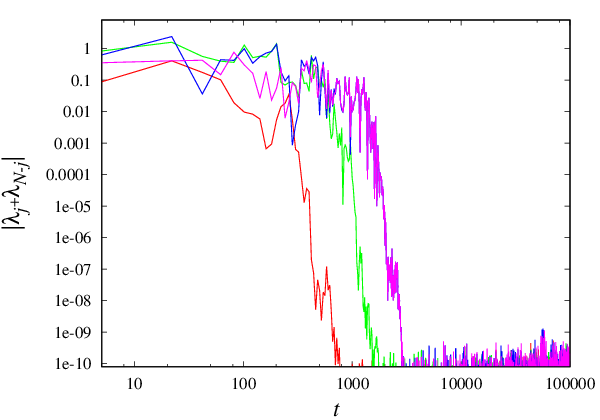
Let us now investigate the initial conditions for the theory, with periodic boundary conditions, at . In Fig. 12, the pairing behavior of the exponents are shown for the initial condition used in [4], , and for a typical random initial condition at the same value of , for comparison. We see that the specific initial condition, Fig. 12 (left), leads to a much longer pairing time, , as compared to few for a random initial condition, which is typical, as can be seen from Table 1. Another apparent feature is that the pairing times for all the pairs are essentially the same in this case, whereas in Fig. 12 (right), they are distinctly ordered in the decreasing order of the absolute value of the Lyapunov exponents.


The reason for the above behavior can be understood as follows. The initial condition leads to a chaotic trajectory, that is restricted to the subspace , as already discussed in Sec. II (Fig. 5). When the trajectory is restricted to this subspace, pairing does not occur. For the fourth order Runge-Kutta integrator with , with the algorithm computing the Lyapunov spectrum, starts to break down visibly at , as seen in Fig. 13 (left). Then the trajectory becomes unrestricted, and within the additional time of few times , the pairing occurs, which is the typical time for pairing seen in Fig. 12 (right). The pairing times in Fig. 12 (left) seem similar for all the pairs, since the difference is roughly an order of magnitude smaller than the time relation breaks down. Once the trajectory is not restricted to the subspace, the pairing occurs, and the Lyapunov exponents converge, as seen in Fig. 13 (right). Computations of the maximal Lyapunov exponent for the trajectory respecting the symmetry results in for [28], which has also been confirmed by our independent calculations. This would conflict with the results in [4], and Fig. 13(right) if the symmetry is unbroken, further adding evidence to the strong possibility that the symmetry was broken in the previous computation[4].
The above consideration brings up another interesting issue: The Lyapunov exponents for the initial conditions , should be those for the trajectory in the subspace . This is the Lyapunov spectrum that is being measured up to in Fig. 13 (right). The Lyapunov exponents averaged over subspaces have been computed for periodic orbits in theory, for example[18]. However, those spectra exhibit pairing behavior. This is intuitively satisfying, since the periodic orbits are symmetric under time reversal. It is unclear if the exponents in the subspace in this case is unpaired, or not converged enough. For the random initial condition in Fig. 12 (right), the Lyapunov exponents start converging from earlier times, as seen in Fig. 13 (right).


Considerations of some technical aspects are in order: The pairing time can depend on the integrator, or its precision, but in an indirect way. To obtain Lyapunov exponents, a trajectory (or trajectories) are integrated over a relatively long time. The numerical accuracy of tracking the trajectory has limitations, especially in a dynamical system with chaos. Since the local Lyapunov exponent depends on the trajectory within the phase space, its pairing behavior is also affected. By varying the time step size in the integrator, , we can control its precision. We studied how the pairing times depends on in Fig. 14. Another technical issue is the ordering of the coordinates within the computation. This affects the local Lyapunov exponents, but does not substantially change the (averaged) Lyapunov exponents, or the pairing time. In Fig. 14 (right), local Lyapunov exponents are shown for the same initial conditions, but with different ordering of the coordinates. The local Lyapunov exponents are similar, but differ in their behavior. The averaged behaviors are compared in Fig. 13 and are shown to be quite similar. So, the technical aspects, as far as we have studied, do not influence the pairing phenomena in an essential way. Considering the results above, when computing Lyapunov exponents, it seems practical to start from a few initial conditions, some perhaps random, since the pairing times, and consequently the convergence time for the Lyapunov exponents can vary significantly.
For the properties of Lyapunov exponents, such as pairing, covariant Lyapunov vectors[29, 30, 31] can potentially provide powerful mathematical tools for their analysis. Their relation to the orthogonal Gram-Schmidt vectors used in this work are known. While outside the scope of this paper, it would be interesting to use these relations to help understand how the pairing times behave. It should be noted, however, that the covariant Lyapunov vectors themselves require computation to obtain, so that it is unclear that it provides an advantage from a practical standpoint.
In this work, we studied symmetry properties, thermodynamic concepts, and the behavior of local Lyapunov exponents in the theory. While seemingly unrelated on the surface, these topics are, as we have seen, closely intertwined. While clarifying some of the issues, questions remain, which we feel attests to the depth and the breadth of the subject.
Acknowledgements.
We would like to thank William Hoover for his encouragement, and discussions. K.A. was supported in part by the Grant–in–Aid for Scientific Research (#15K05217) from the Japan Society for the Promotion of Science (JSPS), and a grant from Keio University.References
- [1] R.C. Hilborn, “Chaos and nonlinear dynamics”, Oxford University Press (New York, 1994).
- [2] M. Tabor, “Chaos and Integrability in Nonlinear Dynamics”, John Wiley & Sons (New York, 1989).
- [3] W.G. Hoover, C.G. Hoover, “Simulation and Control of Chaotic Nonequilibrium Systems”, World Scientific Publishing Company (Singapore, 2015), and references therein.
- [4] Wm. G. Hoover, C. G. Hoover, CMST 23, 73 (2017).
- [5] K. Aoki and D. Kusnezov, Phys. Lett. A 265, 250 (2000); K. Aoki, D. Kusnezov, Ann. Phys. 295, 50 (2002).
- [6] B. Hu, B. Li, and H. Zhao, Phys. Rev. E 61, 3828 (2000).
- [7] Y. Ohnuki and S. Kamefuchi, Phys. Rev. 170, 1279 (1968).
- [8] F. Wilczek, Phys. Rev. Lett. 49, 957 (1982).
- [9] L.Dixon, J.A.Harvey, C.Vafa, E.Witten, Nuc. Phys. B 261, 678 (1985).
- [10] G. ’t Hooft, Nucl. Phys. B 153, 141 (1979).
- [11] W.G. Hoover and K. Aoki, CMST 49, 192 (2017).
- [12] R. Rosenberg, Adv. Appl. Mech., 9, 156 (1966).
- [13] S.W. Shaw, C. Pierre, Journal of Sound and Vibration 150, 170 (1991), ibid. 164 85 (1993).
- [14] K.W. Sandusky and J.B. Page, Phys. Rev. B 50, 866 (1994).
- [15] S. Flach, Physica D 91, 223 (1996).
- [16] A.F. Vakakis, Mech. Sys. Sig. Proc. 11, 3 (1997); Y.V. Mikhlin and K.V. Avramov Appl. Mech. Rev 63, 060802 (2011).
- [17] T. Bountis, G. Chechin and V. Sakhnenko, Int. J. Bif. Chaos 21, 1539 (2011).
- [18] K. Aoki, Phys. Rev. E94, 042209 (2016).
- [19] S. Nosé, J. Chem. Phys. 81, 511 (1984); Mol. Phys. 52, 255 (1984).
- [20] W. G. Hoover, Phys. Rev. A 31,1695 (1985).
- [21] F. Reif, ”Fundamentals of Statistical and Thermal Physics”, Waveland Press (Long Grove, 2009).
- [22] K. Aoki, D. Kusnezov, Phys. Lett. A309, 377 (2003).
- [23] W.H. Press,, S.A. Teukolsky, W.T. Vetterling, B.P. Flannery, “Numerical Recipes: The Art of Scientific Computing, 3rd Edition”, Cambridge University Press (New York, 2007).
- [24] Boost libraries, http://www.boost.org/.
- [25] I. Shimada, T. Nagashima, Prog. Theor. Phys. 61, 1605 (1979).
- [26] G. Benettin, L. Galgani, A. Giorgilli and J. Strelcyn, Meccanica 15, 9 (1980); ibid. 15, 21 (1980).
- [27] H.A. Posch, W.G. Hoover, Phys. Rev. A38, 473 (1988).
- [28] W.G. Hoover, private communication.
- [29] V. Oseledets, Tr. Mosk. Mat. Obs. 19, 179 (1968).
- [30] D. Ruelle,Publ. Math. IHES 50, 275 (1979).
- [31] F. Ginelli, H. Chaté, R. Livi, A. Politi, J. Phys. A: Math. Theor. 46, 254005 (2013).