Channel Estimation with
Systematic Polar Codes
Abstract
Study of polar codes in fading channels is of great importance when applying polar codes in wireless communications. Channel estimation is a fundamental step for communication to be possible in fading channels. For both systematic and non-systematic polar codes, construction of them is based on an information set and the known frozen bits. Efficient implementation of systematic and non-systematic polar codes exists. When it comes to channel estimation or channel tracking, additional pilot symbols are inserted in the codeword traditionally. In this paper, to improve the performance of polar codes in the finite domain, pilot symbols are selected from the coded symbols themselves. In order to keep the existing efficient structure of polar code encoding, pilot selection is critical since not all selections can reuse the existing structure. In this paper, two pilot selections denoted as Uneven Pilot Selection (UEPS) and Even Pilot Selection (EPS) are proposed, which do not change the efficient polar encoding structure. The proposed UEPS and EPS is proven to satisfy the efficient construction condition. The performance of EPS is shown in this paper to outperform both the UEPS and the traditional pilot insertion scheme. Simulation results are provided which verify the performance of the proposed pilot selection schemes.
I Introduction
Polar codes [1], due to the low encoding and decoding complexity of and the capability to realize the capacity of binary-input discrete memoryless channels, are of great potential for future communication applications. The construction of polar code is to select the best bit channels among bit channels to convey information. Besides the binary erasure channel (BEC), polar code construction in all other channel types do not have iterative equations and therefore has a high computation complexity [1, 2, 3, 4, 5].
To improve the error performance of polar codes in the finite domain, successive cancellation list (SCL) decoding is proposed in [6][7] and belief propagation (BP) decoding is applied to polar codes in [8][9][10]. Another direction in improving the error performance of polar codes is to encode systematically instead of the original non-systematic encoding [11]. Systematic polar codes are shown to outperform the non-systematic polar codes in terms of the BER performance with almost no extra cost in the decoding process. Therefore, systematic polar codes are the focus of this paper.
When employing polar codes in a wireless communication scenario, channel state information (CSI) needs to be estimated before further communication is possible. In OFDM and MIMO systems, pilot-aided channel estimation and tracking is studied [12, 13, 14, 15, 16, 17]. Least square (LS) and minimum mean square error (MMSE) channel estimators are commonly used in these works, which are also the estimators in this paper. Pilots are inserted either in the frequency domain or the time domain or in both domains as the LTE systems [18].
In this paper, pilots are not inserted as traditionally done. Instead, pilots are selected from the coded symbols. The motivation behind this pilot selection is to improve the performance of polar codes in the finite domain. The selected pilots not only serve the purpose of channel estimation or tracking, but also provide stronger protection to the information bits during the decoding processing. However, as systematic polar codes can be constructed or implemented efficiently [19][20], the pilot selection scheme in principle should not alter the existing efficient encoding structure. Note that binary phase shift keying (BPSK) is the modulation scheme in this work. Therefore, we interchangeably use pilot symbols, pilot bits, or coded symbols without further noticing.
Let be the generator matrix of the polar code with the block length , and be the set containing the indices of the information bit channels. The submatrix is taken from the matrix with rows and columns both specified by the the set . In this paper, the efficient encoding condition is presented both in our matrix form [19]: and in the domination contiguous form in [20]: the set being domination contiguous (defined in (18)). We prove that the matrix form is equivalent to the set being domination contiguous.
Based on the efficient encoding condition, two pilot selection schemes are proposed: the uneven pilot selection (UEPS) and the even pilot selection (EPS). With pilots selected from the coded symbols, the new encoding set is , where is the set containing pilot symbols selected from the frozen set . The two proposed selections UEPS and EPS are proven to still meet the efficient encoding condition of and the set is proven to be still domination contiguous. The efficiency and decoding performance of the proposed pilot selections are analyzed in the paper. The decoding performance of EPS is analyzed and shown by simulations to be better than the traditional pilot insertion scheme.
The contributions of the paper can be summarized as: 1) The existing two efficient encoding conditions for systematic polar codes [19][20] are proven to be equivalent; 2) Pilots are selected from the coded symbols instead of being inserted additionally. Two pilot selection schemes are proposed which meet the efficient encoding conditions; 3) Theoretical and numerical results are provided which show that the proposed pilot selection scheme outperforms the traditional pilot insertion scheme.
The main notations in this paper are firstly introduced below. A row vector with elements is written as . Given a vector , the vector is a subvector with . If there is a set , then denotes a subvector with elements in .
The rest of the paper is organized as follows. Section II is on the basics of polar codes. It is proven in Section III that the two efficient encoding conditions are essentially the same. In Section IV, two pilot selection schemes are presented and proven to be efficiently encodable. The efficiency and the decoding performance is also analyzed in this section. Simulation results are provided in Section V. Concluding remarks are presented in the last section.
II Polar Code Background
The polarization of independent underlying channels is realized through two stages: channel combining and splitting. Let be the transition probability of . Let be the generator matrix of the polar code with a block length . In [1], the generator matrix is where , is a bit-reversal permutation matrix, and means the th Kronecker power of the matrix in the binary field. Denote as the alphabet set of the input . The channel combining stage produces a vector channel defined as
| (1) |
where .
This vector channel can then be split into bit channels [1]:
| (2) |
Note that the summand in (2) is conditioned on and is summed over to . The channel with the transition probability is the channel that the source bit goes through; it is called bit channel . In the following of the paper, we use to refer to bit channel . Channels are polarized after these two stages in the sense that bits transmitting in these bit channels either experience almost noiseless channels or almost completely noisy channels when is large. The idea of polar codes is to transmit information bits on those noiseless channels. The fixed bits are made known to both the transmitter and receiver.
Mathematically, the encoding is a process to obtain the encoded bits through for a given source vector . The source vector consists of the information bits and the frozen bits, denoted by and , respectively. Here the set includes the indices for the information bits and is the complimentary set. Both sets and are in for polar codes with a block length . The bit channels in are better than those in . Or in other words, the bit channels in should be stochastically degraded with respect to those in .
For two bit channels and , denote if bit channel is stochastically degraded with respect to bit channel as [3]. In mathematical terms, the information set for the underlying channel has the following property:
| (3) |
Denote the size of as . In this paper, suppose the set is found from calling any sorting algorithm such as [3]. The frozen bits in are fixed bits which are made known to the receiver.
The systematic polar code [11] is constructed by specifying a set of indices of the codeword as the indices to convey the information bits. Denote this set as and the complementary set as . The codeword is thus split as . With some manipulations, we have
| (4) |
The matrix is a submatrix of the generator matrix with elements . The vector can be obtained as the following
| (5) |
From (5), it is seen that is one-to-one if the following two conditions are met:
| (6) | |||
| (7) |
In [11], it is shown that satisfies these two conditions in order to establish the one-to-one mapping . In the rest of the paper, the systematic encoding of polar codes adopts this selection of to be . Therefore we can rewrite (4) as
| (8) |
Remark: In the context of the systematic polar codes, it is convenient to refer to the generator matrix as the one without permutation, namely . The equation (8) is established under this matrix without permutation. From now on, the matrix is in this form without the permutation matrix unless stated otherwise.
The successive cancellation (SC) decoding of polar codes is proposed in [1], which has a low complexity of . The decision statistic of the SC decoder is:
where
The bits are decoded in the order from 1 to . One bit error in will propagate to the information bit with . This results in an non-satisfactory performance of polar codes in the finite domain [9, 21, 22, 10].
III Efficient Construction of Polar Codes
The systematic mapping in (8) can be simplified as in [19] from the fact that . Here we provide another proof of which is a simplified version of the one cited from [19].
Proposition 1
For a polar code with an information set as defined in (3), the submatrix of is a zero matrix: .
Proof:
Let be the binary expansion of the index of bit channel (). The bit channel and is said to have a binary domination relation if
| (15) |
From the definition of the generator matrix , it is shown in [1] and [20] that if and only if , meaning the support of contains the support of . Let and . If , then we have . From [2] and [20], the binary domination of and indicates bit channel upgradation: . But this contradicts with the fact that bit channel is statistically degraded to all bit channels in the information set . Therefore has to be zero. ∎
As in [11], systematic encoding of polar codes adopts the selection of . Efficient implementation of systematic codes exists [19][20]. In [19], the efficient construction of systematic polar codes resides on the fact that in the binary field. In [20], this condition is reformed as information set being domination contiguous: for , and for , the following holds:
| (18) |
We now prove that the conditions in [19] and [20] are essentially the same.
To prove the equivalence of the two efficiently encodable conditions in [19] and [20], the notations in [20] are introduced below. Let the information bit channel set be an ascending ordered set. Define a matrix (with a size of by ) as
Let us first look at an example of this matrix . Suppose and . Then is
In [20], with being domination contiguous, the matrix is proven to be an involution:
| (22) |
where is the identity matrix. This is the basis for the efficient structure of systematic encoding for polar codes in [20]. The following proposition shows that the condition in (22) is essentially the same as the efficient encoding condition in [19].
Proposition 2
The condition obtained from being domination contiguous is equivalent to .
Proof:
First note that the generator matrix . The operation is then . From the definition of in (III), the result of is to take the rows in from the matrix , denoted as . Then . Similarly, the operation of is taking columns of , which indicates that . Therefore, the condition is equivalent to . ∎
From (16) and (17) and that [19], can be solved directly without going through the structure related to . What’s more important is that the non-systematic and the systematic encoding structure is essentially the same because . Such systematic selection is considered as efficiently encodable. In the sequel, we discuss pilot selections which satisfy the efficiently encodable condition:
| (23) |
IV Pilot Selection Schemes
The general pilot selection needs to meet the channel estimation requirements. In an OFDM system, channel estimation can be done by setting some of the sub-carriers to be pilots to account for the frequency variation of the channel. In the mean time, wireless channels can be time varying. Therefore, pilots in the time domain are also inserted. To make tradeoff between transmission efficiency and channel estimation accuracy, pilots are often sparsely inserted in the frequency or the time domain [18]. In this section, the transmission model of this paper is first introduced and then pilot selections are discussed.
IV-A Transmission Model
In this section, the transmission model is discussed. The encoded binary bits in is transmitted through the underlying channel . Denote a matrix as a diagonal matrix with elements taken from the codeword . The received signal is then
| (24) |
where is the channel response for each coded symbol and is the AWGN noise vector with each element having mean zero and variance . Assume there is no inter-symbol interference (ISI) in this model. In this paper, the channel is assumed to follow the Rayleigh distribution with a Doppler shift . With Jake’s spectrum, the time correlation of the channel can be described by the first kind of 0-th order Bessel function:
| (25) |
where is the autocorrelation function of the channel and is the symbol duration. In the next subsections, pilot selections are discussed in order to estimate the channel .
IV-B Efficient Selection Criterion
Denote as pilot positions in and as the pilot positions in . Then are known pilot symbols. The encoding of polar codes with pilot selections is equivalent to the following problem: for each information vector and the construction conditions: , , how to calculate in order to produce ? One can immediately observe that this problem has no solution since the linear equation behind (17) only needs a length vector . However, in the pilot selection case, there are additional known values in . Note that the known pilots are imbedded in the information bits . The new encoding problem with pilots in is therefore less constrained. Fig. 1 shows such an encoding problem with and . In Fig. 1 two pilots are selected: symbol 3 and symbol 6. Symbol 3 is from the set and symbol is in the information set . Therefore, there are 5 known values from the right-hand side while only 4 unknowns () are required in the original systematic encoding of polar codes.

To make the encoding problem render a unique solution, one has to add more constraints. Specifically, constraints are needed. This means some of the frozen bits in can not be frozen anymore. Let the union of the information set and the pilots in be . The encoding procedure can now be expressed as:
| (26) |
One important note about this new encoding with pilot selection is that the set is no longer the information set as in the original encoding in (8). Instead, it includes elements in from the definition of . Therefore, the validity of this new encoding needs to be first verified. Then the efficient encodable mapping needs to be established.
The first condition of a valid mapping in (6) is trivial: has the same elements as . The second condition (7) is that the mapping is one-to-one or is invertible. This condition can also be easily verified as in [11]: is lower triangular with 1s at the diagonal and is therefore invertible.
Now comes to the efficient construction of this new selection in (26). It is already pointed out in Section III that the efficient construction relies on the fact that . The following lemma shows that this condition is met if .
Lemma 1
Let . When , then .
Proof:
The proof is as in [19]. With , in (26) can be written as
| (27) |
which is equivalent as:
| (28) |
as is an invertible matrix (being a lower triangular matrix with ones at the diagonal). In the mean time, from the encoding process and [19], we have
| (29) |
Decompose the vector in (29) as:
| (30) |
Since is an invertible matrix, (28) and the first part of (30) is equivalent as: = in the binary field. ∎
From Lemma 1, the efficient construction condition can be checked from the submatrix . Note that this condition from Lemma 1, unlike the condition in [19] or [20], does not involve matrix inversion or matrix multiplication. Therefore is a simplified working condition to check whether a selection is efficiently encodable. In the rest of the paper, is used to check the proposed pilot selection schemes to determine whether they are efficiently encodable.
Compared with the submatrix , has less rows but more columns. With containing elements in , is not guaranteed to be an all-zero matrix. In other words, the proof in [19] is not applicable for . The set is not necessarily domination contiguous.
However, this efficient encodable problem is still promising due to the special or the sparse nature of the generator matrix . In the next two sections, we propose two pilot selections which are efficiently encodable. Before going further, the following lemma is immediately available.
Lemma 2
Let where . Compared with , all increased columns of are from .
Proof:
The complementary set of has less elements compared with : (Here is the excluding operation). The submatrix is
| (31) | |||||
| (32) |
The first part of (32): , has the same columns as . The second part of (32): contains the additional columns of . Since and , the matrix is from . Therefore, compared with , the additional columns of are from . ∎
IV-C Uneven Pilot Selection (UEPS)
The matrix is an invertible matrix: it is a lower-triangular matrix with ones at the diagonal in the binary field. A detailed observation of reveals that some of the columns are all zeros except the diagonal elements. Denote as the Hamming weight of the inside argument. The following set is defined over as:
| (33) |
where is the th column of the submatrix . Remember that, as in the proof of Proposition 2, is a submatrix formed by taking rows of . The following selection of pilots yields an efficiently encodable scheme.
Proposition 3
Uneven Pilot Selection (UEPS): Let and the pilots in the set can be any desired selections. Then yields .
Proof:
Since , the first part of (32): from Proposition 1. Now consider the second part of (32). The rows and columns of the matrix are from the set . Since the matrix is a lower triangular matrix with ones at the diagonal, the columns of possess ones at the diagonal and are zeros elsewhere. With , the non-zero elements surely only appear at the diagonal positions. However excludes these diagonal positions. Therefore . According to Lemma 2, this means . ∎
With Lemma 1, the selection in Proposition 3 meets the efficiently encodable condition in (23) and is therefore an efficiently encodable selection. Take and as an example. The encoding process selects the information set as and the frozen set is . The submatrix is provided below:
Note that the last column (column eight) of is actually column nine of . Other columns of correspond to the same columns of . Then, from the submatrix , the set can be obtained as . If , then .
Given the pilot selection as in Proposition 3, it is of interest to link it with the domination contiguous condition in [20]. The following proposition shows that the pilot selection in Proposition 3 produces a domination contiguous set .
Proposition 4
The set where is domination contiguous.
However the pilots selected according to Proposition 3 can not be evenly distributed among bit channels to . The pilot positions are dependent on the information set . For the same block length and code rate, different channel conditions produce different information sets . This makes the pilot selection inconsistent among channels and therefore can not be flexibly configured. These drawbacks motivate us to explore the structure of the encoding matrix to find controllable pilot selections which are not dependent on the information set .
IV-D Even Pilot Selection (EPS)
Before the introduction of the pilot selection in this section, a new set is defined as
| (34) |
The submatrix of is an all-zero matrix as stated in the following proposition.
Proposition 5
With defined in (34), the submatrix of is an all-zero matrix: .
Proof:
The generator matrix is where . The matrix can be decomposed as:
| (35) |
Observe the matrix :
| (36) |
The fourth column of has one non-zero element at the fourth position. Now extracting the submatrix of by selecting the columns specified by the set in (34). Denote as such a matrix. From the expression of in (35) and that only the fourth element of the fourth column of is non-zero, it can be immediately concluded that the non-zero elements of only appear in rows specified by the set . In other words, . ∎
For a given information set , let and . The following proposition states the second pilot selection which is efficiently encodable.
Proposition 6
Even Pilot Selection (EPS): Let be the set containing any desired pilots in the information set , and the pilots in the frozen set is: . Then with the set , the submatrix .
Proof:
Since in this selection, equation (32) can be rewritten as
| (37) |
With and , the first part of (37) is therefore an all-zero matrix: . The second part of (37): contains the additional columns of compared with . Since , then . With
| (38) | |||
| (39) |
it can be immediately shown that
| (40) | |||
| (41) |
Then the matrix is a submatrix from . From Proposition 6, . Therefore . Since the first part of (37) is an all-zero matrix and , the submatrix is therefore an all-zero matrix. ∎
Applying Lemma 1, the selection in Proposition 6 is also an efficiently encodable selection because it meets the condition in (23). This selection does not depend on the distribution of the set . The candidates of the pilots are always fixed () for a given block length . The only requirement of this selection is to make sure all the elements in are selected as pilots.
Fig. 2 shows the pilots selected for polar codes with and . The underlying channel is the AWGN channel with an of dB (BPSK is applied here). There are total 64 pilots selected for both UEPS and EPS. In EPS, the pilots from the information set is . From Fig. 2, the pilots selected from Proposition 3 (UEPS) are not evenly distributed while pilots from Proposition 6 (EPS) is guaranteed to be evenly distributed. For UEPS, if the number of elements of the set is less than the number of pilots to be selected, then pilots from the information set can be selected to be evenly distributed. The pilots of UEPS in Fig. 2 are selected in such a way. However, even with this optimization, there are still gaps between pilots observed for UEPS in Fig. 2. On the other hand, the integer multiples of can be selected as pilots when needed in EPS. Therefore, the channel estimation performance of EPS in general should be better than that of UEPS.

To conclude this section, we want to point out that the set is domination contiguous.
Proposition 7
The set is domination contiguous.
IV-E Efficiency Comparison with Traditional Pilot Insertion
The two pilot selections in the previous two subsections are to use the coded symbols as pilots. Traditional pilots are inserted into the existing codewords. For example, in LTE, downlink pilots are inserted every four symbols in the time domain [18]. Fig. 3 shows a comparison of EPS pilot selection and the traditional pilot insertions.


Suppose on average pilots are needed in one polar code block. For UEPS and EPS pilot selections, denote where is the number of pilots in the information set and is the number of pilots in the frozen set . The equivalent throughput of UEPS and EPS is therefore:
| (42) |
The equivalent throughput of the traditional pilot insertions is:
| (43) |
Assume the pilots are selected or inserted with an even spacing (which is the case for many practical systems). Let , where is the ratio of pilots selected or inserted in one code block. With the even spacing assumption, . With simple manipulations, the ratio of is:
| (44) |
Remark: This ratio of only works for EPS in Section IV-D relative to the traditional pilot insertion. UEPS in Section IV-C does not have an evenly distributed pilots and therefore violates the assumption of the even spacing between pilots. Also note that the ratio in (44) does not depend on the block length or the code rate . It is only dependent on the ratio : the fraction of pilots selected or inserted in one code block.
Fig. 4 shows the ratio with some values of . Pick a typical value of , the ratio , meaning that EPS in Section IV-D only has a slightly smaller throughput compared with the traditional pilot insertion. However, as analyzed in the next subsection and from the simulation results in Section V, the performance of EPS is much better than that of the traditional pilot insertion. Furthermore, the small throughput loss of UEPS and EPS can be overcome by initially setting a larger code rate than that of the traditional pilot insertion. In Section V, with the same throughput between EPS and the traditional pilot insertion, EPS still has a very clear advantage in terms of the error performance.

IV-F Decoding Processing with Pilot Selections
The error performance of the pilot selections is the main motivation of this paper. Bear in mind that, the traditional inserted pilots only facilitate the channel estimation. The proposed pilot selections UEPS and EPS not only serve the purpose of channel estimation, but also help in the decoding process. Fig. 5 shows the log likelihood ratio (LLR) values fed from the left-hand side and the right-hand side of the decoding graph. The parameters of the polar code in Fig. 5 is the same as that in Fig. 1 where , and two symbols, and , are selected as pilots. Assume pilot symbols are all zeros. Then the LLR values corresponding to the pilot symbols can be set to infinity in the decoding process.
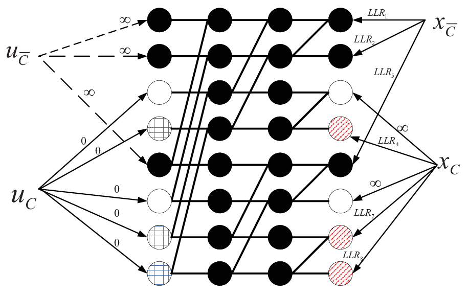
Polar code decoding, be it the original successive cancellation (SC) decoding or the belief propagation (BP) decoding, can be unified in the BP decoding frame [9]. Also bear in mind that the generator matrix is an involution: . The involution property of the matrix can be interpreted as the following: a LLR value fed from the left-hand side propagates through the same nodes and edges as that fed from the same position from the right-hand side and therefore has the same contribution to the decoding performance. For a given block length and code rate , the decoding performance of polar codes can now be characterized by the initial conditions set
| (45) | |||||
where the vector contains the received samples from the channel and is the LLR values of the inside arguments. Apparently, when no symbols are selected as pilots, there are frozen bits () and the LLRs corresponding to the information bits are .
When analyzing the effect of pilot selections to the decoding performance, the pilots in the frozen set and pilots in have to be differentiated. First let us look at the pilots in the frozen set . Without loss of generality, take EPS in Section IV-D as an example. For any , a corresponding in the left-hand side is taken from the frozen set , which results in a zero LLR value fed from the left-hand side to the decoding graph. This conversion of from the frozen bit to a non-frozen bit is a basic requirement of the new encoding process in Section IV-B. The symbol in Fig. 5 is such an example: in the decoding process, the LLR of (the received sample of ) is fixed as infinity while the LLR of is 0. The initial condition set is now:
| (46) | |||||
Comparing the set with the set in (45), the infinite LLR values feeding into the decoding diagram is the same: there are additional infinite LLR values from the right-hand side but less infinite LLR values from the left-hand side. Therefore, the decoding error performance of polar codes given the input set and should be on the same level. In this case, we consider and as equivalent.
When a symbol is selected as a pilot, the decoding performance is improved compared when symbol is a normal information bit. Since and are equivalent, here we only select as pilots. The new initial set is
| (47) |
Note that the initial is merged with as in (47). The initial condition set with pilots selected from has additional infinite LLR values compared with the set in (45). These are stronger (or absolutely definite) initial values which greatly benefit the decoding process. In this sense, the decoding performance of the EPS scheme with at least one pilot from the information set should be better than the traditional pilot insertion with the same number of pilots inserted. The simulation results in Section V verified the analysis in this section.
IV-G Channel Estimation Performance
The channel estimation performance in terms of mean square error (MSE) is analyzed in this section. Two estimators are used in this paper: least square (LS) and minimum mean square error (MMSE) estimators. Then linear interpolation is used to estimate the channel response at non-pilot positions. Let the set be the set containing all the pilot positions. For the LS estimator, the estimation of the channel response at the pilot positions are [17] [23]
| (48) |
The MSE of the LS estimator is well established to be:
| (49) |
While for the MMSE estimation, the estimation of the channel response at the pilot positions are:
| (50) |
where the matrix is the cross correlation of the vector and : and is the identity matrix. Without simplifications and approximations, the MSE of the estimation does not in general yield a closed form expression. However, as shown in [17] [23], MMSE performs better than LS in low regions. Numerical results of the MSE of EPS and UEPS with MMSE and LS are reported.
The pilot selection UEPS or EPS should have the same channel estimation performance as the traditional pilot insertion given that pilots are inserted in the same positions as UEPS or EPS. However, UEPS in general should have worse channel estimation performance than EPS due to the uneven nature of its pilots. In the next section, the MSE performance of these schemes are compared.
Remark: When the channel responses are highly correlated (for example, in a static or a slowly moving environment), the pilots (from the information set) of EPS (or UEPS) can be made more sparse to increase the throughput, while the pilots can still be (or in (33)) (these pilots do not affect the overall throughput). In a fast-moving environment (with large Doppler frequencies), although (or ), can be made as dense as needed. Actually, one pilot every four symbols of EPS is already a very dense selection which should be able to meet requirements of most applications.
V Numerical Results
In this section, the pilot selections in Section IV are simulated. The channel is assumed to be the Rayleigh fading channel. Two channel estimators are compared: Least Square (LS) and Minimum Mean Square Error (MMSE). Linear interpolation is used to estimate the channel at non-pilot positions. The polar code simulated has block length . The encoded symbols are modulated with the BPSK scheme. The SC decoding is applied in the decoding process. The following wireless scenario is selected as a test case: the carrier frequency is MHz and the symbol rate is Ksps. Two Doppler frequencies Hz and Hz are tested in this section, corresponding to two velocities of km/h and km/h, respectively. The information set is selected from the Tal-Vardy algorithm in [3] with an of dB (a further increase of the construction does not improve the error performance).
The MSE of the estimators is compared in Fig. 6 where the code rate is . As expected, for EPS, the LS estimator is not as good as the MMSE estimator. With the MMSE estimator, the EPS scheme outperforms the UEPS scheme, also as expected from the discussions in Section IV-G: the pilots in UEPS are not evenly distributed as EPS. The MSE performance of UEPS is almost the same as that of the EPS scheme with the LS estimator. In the following results, the decoding performance echoes this observation.
The frame-error-rate (FER) performance of the EPS in Section IV-D is shown in Fig. 7. The pilots selected are: and . The initial code rate of the polar code is . Remember that and contains elements (multiples of four) in the frozen and information set, respectively. From Fig. 7, it can be seen that the MMSE method with Hz has a better FER performance than that of the LS with the same Doppler shift. When goes up to Hz, the FER performance of MMSE and LS is worse than the corresponding performance at Hz.
The performance of the pilot selection UEPS in Section IV-C is compared with that of EPS in Fig. 8. Note that pilots selected for UEPS are done in two steps. First, the pilots in (33) are selected from the frozen set . Then, the remaining pilots are selected from the information set . To achieve the best interpolation results, the pilots of UEPS in are evenly selected. Both EPS and UEPS have 64 pilots with 40 of them selected from the information set. The Doppler shift in the simulation of Fig. 8 is Hz. The EPS with MMSE is better than UEPS with MMSE: at the FER of , UEPS with MMSE requires 2 dB more than EPS with MMSE. For UEPS and EPS with LS, similar phenomenon is observed. The superior performance of EPS pilot selection is due to the even distribution of pilots rather than the unevenly distributed pilots in UEPS.
The two efficient pilot selections UEPS and EPS are compared with the traditional pilot insertion in Fig. 9 where the Doppler shift is also Hz. For the pilot insertion scheme, pilots are evenly inserted: one pilot is inserted every four coded symbols. The polar code used for the pilot insertion has a block length and an initial code rate . The number of pilots in these three schemes are the same: total pilots are employed. According to the analysis in Section IV-E, the overall throughput of the traditional pilot insertion is . To maintain the same throughput of UEPS and EPS as that of the traditional pilot insertion, the initial code rate of the polar code is adjusted as . Among the pilot symbols, of them are from , resulting in a final throughput of for both UEPS and EPS schemes. It can be seen from Fig. 9 that the UEPS and the traditional pilot insertion has almost the same FER performance when MMSE is applied while EPS has a better FER performance. Thus the 2 dB advantage of EPS over UEPS at FER applies to the traditional pilot selection. However, this advantage of EPS over the traditional pilot insertion comes from the fact that all pilots inserted only serve as the channel estimation elements. For EPS pilot selection, the pilots also facilitate the decoding of polar codes as discussed in Section IV-F.


VI Conclusion
In this paper, two pilot selection schemes, uneven pilot selection (UEPS) and even pilot selection (EPS) are studied for polar codes in fading channels. By selecting coded symbols as pilots, instead of inserting pilots, the decoding performance of polar codes is greatly improved. Considering the unsatisfactory performance of polar codes in the finite domain, the proposed pilot selection scheme EPS can be employed in practical systems for channel estimation or tracking. Simulation results show that the proposed EPS scheme outperforms both the UEPS scheme and the traditional pilot insertion scheme and therefore is a promising option to improve the polar code performance in wireless communications.
Appendix A Proof of Proposition 4
Let .
- •
If , then any which satisfies and must be in since is domination contiguous [20]. In this case, .
- •
If and , when satisfying and , then . When satisfying and , then from the selection of and the definition of in (33), it can be concluded that there is no other elements in which satisfy except . Therefore .
- •
If , there is no which meets since bit channel is worse than bit channel and therefore can never occur. If , then has to be the same as in order to have .
- •
If and , to have , then has to be from . To have , has to be from . There is no to satisfy and .
From the above analysis, for all , the s which meet and are also in . This concludes that is domination contiguous.
Appendix B Proof of Proposition 7
The proof of this proposition is similar to Appendix A. Let .
- •
If , then any which satisfies and must be in since is domination contiguous [20]. In this case, .
- •
If and , when satisfying and , then . When satisfying and , then the binary expansion of can be expressed . The last two bits are ones since is a multiple of 4 and . The number with is again a multiple of 4. Therefore .
- •
If , there is no which meets since bit channel is worse than bit channel and therefore can never occur. If , then has to be a multiple of 4 in order to have . In this case .
- •
If and , to have , then has to be from . To have , has to be from . There is no to satisfy and .
From the above analysis, for all , the s which meet and are also in . This concludes that is domination contiguous.
References
- [1] E. Arikan, “Channel Polarization: A Method for Constructing Capacity-Achieving Codes for Symmetric Binary-Input Memoryless Channels,” IEEE Transactions on Information Theory, vol. 55, no. 7, pp. 3051–3073, 2009.
- [2] R. Mori and T. Tanaka, “Performance of polar codes with the construction using density evolution,” IEEE Communications Letters, vol. 13, no. 7, pp. 519–521, Jul. 2009.
- [3] I. Tal and A. Vardy, “How to Construct Polar Codes,” Information Theory, IEEE Transactions on, vol. 59, no. 10, pp. 6562–6582, Oct 2013.
- [4] P. Trifonov, “Efficient Design and Decoding of Polar Codes,” IEEE Transactions on Communications, vol. 60, no. 11, pp. 3221–3227, November 2012.
- [5] D. Wu, Y. Li, and Y. Sun, “Construction and Block Error Rate Analysis of Polar Codes Over AWGN Channel Based on Gaussian Approximation,” IEEE Communications Letters, vol. 18, no. 7, pp. 1099–1102, Jul. 2014.
- [6] K. Chen, K. Niu, and J. Lin, “Improved Successive Cancellation Decoding of Polar Codes,” IEEE Transactions on Communications, vol. 61, no. 8, pp. 3100–3107, August 2013.
- [7] I. Tal and A. Vardy, “List Decoding of Polar Codes,” Information Theory, IEEE Transactions on, vol. 61, no. 5, pp. 2213–2226, May 2015.
- [8] E. Arikan, “A Performance Comparison of Polar Codes and Reed-Muller codes,” IEEE Communications Letters, vol. 12, no. 6, pp. 447–449, 2008.
- [9] N. Hussami, S. Korada, and R. Urbanke, “Performance of Polar Codes for Channel and Source Coding,” in IEEE International Symposium on Information Theory (ISIT), June 2009, pp. 1488–1492.
- [10] J. Guo, M. Qin, A. G. i Fabregas, and P. H. Siegel, “Enhanced Belief Propagation Decoding of Polar Codes through Concatenation,” in 2014 IEEE International Symposium on Information Theory Proceedings (ISIT), 2014, pp. 2987 – 2991.
- [11] E. Arikan, “Systematic Polar Coding,” IEEE Communications Letters, vol. 15, no. 8, pp. 860–862, August 2011.
- [12] Y. Li, “Pilot-symbol-aided channel estimation for ofdm in wireless systems,” IEEE Transactions on Vehicular Technology, vol. 49, no. 4, pp. 1207–1215, Jul 2000.
- [13] M. Morelli and U. Mengali, “A Comparison of Pilot-Aided Channel Estimation Methods for OFDM Systems,” IEEE Transactions on Signal Processing, vol. 49, no. 12, pp. 3065–3073, December 2001.
- [14] Y. Li, “Simplified channel estimation for ofdm systems with multiple transmit antennas,” IEEE Transactions on Wireless Communications, vol. 1, no. 1, pp. 67–75, Jan 2002.
- [15] K. J. Kim, J. Yue, R. A. Iltis, and J. D. Gibson, “A qrd-m/kalman filter-based detection and channel estimation algorithm for mimo-ofdm systems,” IEEE Transactions on Wireless Communications, vol. 4, no. 2, pp. 710–721, March 2005.
- [16] H. Minn, N. Al-Dhahir, and Y. Li, “Optimal training signals for mimo ofdm channel estimation in the presence of frequency offset and phase noise,” IEEE Transactions on Communications, vol. 54, no. 10, pp. 1754–1759, Oct 2006.
- [17] M. Biguesh and A. B. Gershman, “Training-based mimo channel estimation: a study of estimator tradeoffs and optimal training signals,” IEEE Transactions on Signal Processing, vol. 54, no. 3, pp. 884–893, March 2006.
- [18] 3rd Generation Partnership Project (3GPP TM), “Technical Specification Group Radio Access Network; Evolved Universal Terrestrial Radio Access (E-UTRA); Physical Channels and Modulation (Release 10) ,” 3GPP TS 36.211 V10.7.0 (2013-02).
- [19] L. Li and W. Zhang, “On the Encoding Complexity of Systematic Polar Codes,” in IEEE International System-on-Chip Conference (SOCC), Sep 2015, pp. 508–513.
- [20] G. Sarkis, I. Tal, P. Giard, A. Vardy, C. Thibeault, and W. J. Gross, “Flexible and Low-Complexity Encoding and Decoding of Systematic Polar Codes,” IEEE Transactions on Communication, vol. 64, no. 7, pp. 2732–2745, June 2016.
- [21] A. Eslami and H. Pishro-Nik, “On Bit Error Rate Performance of Polar Codes in Finite Regime,” in 48th Annual Allerton Conference on Communication, Control, and Computing (Allerton), 2010, pp. 188–194.
- [22] ——, “A Practical Approach to Polar Codes,” in IEEE International Symposium on Information Theory, 2011, pp. 16–20.
- [23] Y. S. Cho, J. Kim, W. Y. Yang, and C. G. Kang, MIMO-OFDM Wireless Communications with Matlab. John Wiely & Songs (Asia) Pte Ltd, 2010.
![[Uncaptioned image]](1801.02860v1/picture_L.png) |
Liping Li (S’07-M’15) is now an associate professor of the Key Laboratory of Intelligent Computing and Signal Processing of the Ministry of Education of China, Anhui University, Hefei, China. She got her PhD in Dept. of Electrical and Computer Engineering at North Carolina State University, Raleigh, NC, USA, in 2009. Her current research interest is in channel coding, especially polar codes. Dr. Li’s research topic during her PhD studies was multiple-access interference analysis and synchronization for ultra-wideband communications. Then she worked on a LTE indoor channel sounding and modeling project in University of Colorado at Boulder, collaborating with Verizon. From 2010 to 2013, she worked at Maxlinear Inc. as a staff engineer in the communication group. At Maxlinear, she worked on SoC designs for the ISDB-T standard and the DVB-S standard, covering modules on OFDM and LDPC. In Sept. 2013, she joined Anhui University and started her research on polar codes until now. |
![[Uncaptioned image]](1801.02860v1/picture_X.png) |
Zuzheng Xu (S’17) is currently pursuing the M.S. degree in the School of Electronics and Information Engineering, Anhui University. His research interest is in polar codes. Specifically, he is interested in improving polar code performance in wireless fading channels. |
![[Uncaptioned image]](1801.02860v1/picture_H.png) |
Yanjun Hu (SM’07) is a professor of the Key Laboratory of Intelligent Computing and Signal Processing of the Ministry of Education of China, Anhui University, Hefei, China. She is a senior member of IEEE. Dr. Hu got her PhD in Communications and Information System in 1998 from University of Science and Technology of China. . She was a visiting scholar from Feb. 2005 to Aug. 2006 in University of Ottawa, Canada. Dr. Hu’s research covers wireless communications and wireless sensor networks. She’s published over one hundred research papers and holds three patents. She has funded by NSFC and other key projects in China. |