A Mixed Finite Element Method for Multi-Cavity Computation in Incompressible Nonlinear ElasticityThanks: The research was supported by the NSFC projects 11171008 and 11571022.

Weijie Huang Zhiping Li ^†^†thanks: Corresponding author, email: lizp@math.pku.edu.cn Affiliation: LMAM & School of Mathematical Sciences, Peking University, Beijing 100871, China

Abstract

A mixed finite element method combining an iso-parametric $Q_{2}$ - $P_{1}$ element and an iso-parametric $P_{2}^{+}$ - $P_{1}$ element is developed for the computation of multiple cavities in incompressible nonlinear elasticity. The method is analytically proved to be locking-free and convergent, and it is also shown to be numerically accurate and efficient by numerical experiments. Furthermore, the newly developed accurate method enables us to find an interesting new bifurcation phenomenon in multi-cavity growth.

Key words: multiple cavitation computation, incompressible nonlinear elasticity, mixed finite element method, locking-free, convergent

1 Introduction

Cavitation phenomenon, which exhibits sudden dramatic growth of pre-exist small voids under loads exceeding certain criteria, is first systematically modeled and analyzed by Gent & Lindley [1] in 1958. It is considered one of the most important failure phenomenon in nonlinear elasticity, and its better understanding is crucial to explore the properties of elastic materials.

Let $\Omega\subset\mathbb{R}^{n}\,(n=2,3)$ be a simply connected domain with sufficiently smooth boundary $\partial\Omega$ , and let $B_{\rho_{k}}(\bm{x}_{k})=\{\bm{x}\in\mathbb{R}^{n}:|\bm{x}-\bm{x}_{k}|<\rho_{k}\}$ and $\bigcup_{k=1}^{K}B_{\rho_{k}}(\bm{x}_{k})\subset\Omega$ . Let $\Omega_{\rho}=\Omega\setminus\bigcup_{k=1}^{K}B_{\rho_{k}}(\bm{x}_{k})$ be the domain occupied by an elastic body in its reference configuration, where $B_{\rho_{k}}(\bm{x}_{k})$ denotes the pre-existing defects of radii $\rho_{k}\ll 1$ centered at $\bm{x}_{k}$ , $k=1,\cdots,K$ . Then, in incompressible elastic materials, the multi-cavitation problem can be expressed as to find a deformation $\bm{u}$ to minimize the total energy

E(\bm{u})=\int_{\Omega_{\rho}}W_{0}(\nabla\bm{u}(\bm{x}))\,\mathrm{d}\bm{x},

(1.1)

in the set of admissible deformation functions

\mathcal{A}_{I}=\{\bm{u}\in W^{1,s}(\Omega_{\rho};\mathbb{R}^{n})\ \mbox{is 1-to-1 a.e.}:\bm{u}|_{\partial\Omega}=\bm{u}_{0},\;\det\nabla\bm{u}=1,\mbox{ a.e.}\},

(1.2)

where $W_{0}:M^{n\times n}_{+}\rightarrow\mathbb{R}^{+}$ is the stored energy density function of the material with $M_{+}^{n\times n}$ being the set of $n\times n$ matrices of positive determinant, and $n-1<s<n$ is a given Sobolev index, and where a displacement boundary condition $\bm{u}=\bm{u}_{0}$ is imposed on $\partial_{D}\Omega_{\rho}=\partial\Omega$ , and a traction free boundary condition is imposed on $\partial_{N}\Omega_{\rho}=\cup_{k=1}^{K}B_{\rho_{k}}(\bm{x}_{k})$ . Without loss of generality, we consider a typical energy density for nonlinear elasticity given as

\displaystyle W(F)=\mu|F|^{s}+d(\det F),\quad\forall F\in M_{+}^{n\times n},

(1.3)

where $\mu$ is material parameter, and $d(\det F)=\kappa(\det F-1)^{2}+d_{1}(\det F)$ with $\kappa>0$ and $d_{1}:\mathbb{R}_{+}\to\mathbb{R}_{+}$ being a strictly convex function satisfying

\displaystyle d_{1}(\xi)\to+\infty\ \text{as}\ \xi\to 0,\ \text{and}\ \dfrac{d_{1}(\xi)}{\xi}\to+\infty\ \text{as}\ \xi\to+\infty.

(1.4)

Notice that, even though for incompressible nonlinear elastic materials, $d(\cdot)$ is just a constant as the determinant of any admissible deformation in $\mathcal{A}_{I}$ equals 1 a.e., the term plays an important role in the proof of the convergence of the numerical cavitation solutions to the mixed formulation given below.

To relax the rather restrictive condition $\det\nabla\bm{u}=1,\mbox{ a.e.}$ appeared in $\mathcal{A}_{I}$ , a mixed formulation of the following form (see [9, 2]) is usually used in computation:

(\bm{u},p)=\arg\sup_{p\in L^{2}(\Omega_{\rho})}\inf_{\bm{u}\in\mathcal{A}}E(\bm{u},p),

(1.5)

where $p\in L^{2}(\Omega_{\rho})$ is a pressure like Lagrangian multiplier introduced to relax the constraint of incompressibility, and where the Lagrangian functional $E(\bm{u},p)$ and the set of admissible deformations $\mathcal{A}$ are defined as

\displaystyle E(\bm{u},p)=\int_{\Omega_{\rho}}\left(W(\nabla\bm{u})-p\left(\det\nabla\bm{u}-1\right)\right)\,\mathrm{d}\bm{x},

(1.6)

\mathcal{A}=\{\bm{u}\in W^{1,s}(\Omega_{\rho};\mathbb{R}^{n})\ \mbox{is 1-to-1 a.e.},\bm{u}|_{\partial_{D}\Omega_{\rho}}=\bm{u}_{0}\}.

(1.7)

The nonlinear saddle point problem (1.6)-(1.7) with energy density (1.3) leads to the mixed displacement/traction boundary value problem of the Euler-Lagrange equation:

$\displaystyle\operatorname{div}\big(D_{F}W(\nabla\bm{u})-p\operatorname{cof}\nabla\bm{u}\big)$	$\displaystyle=$	$\displaystyle 0,\ \quad\text{in}\,\,\,\Omega_{\rho},$	(1.8)
$\displaystyle\det\nabla\bm{u}$	$\displaystyle=$	$\displaystyle 1,\ \quad\text{in}\,\,\,\Omega_{\rho},$	(1.9)
$\displaystyle\big(D_{F}W(\nabla\bm{u})-p\operatorname{cof}\nabla\bm{u}\big)\bm{n}$	$\displaystyle=$	$\displaystyle\bm{0},\ \quad\text{on}\ \cup_{k=1}^{K}\partial B_{\rho_{k}}(\bm{x}_{k}),$	(1.10)
$\displaystyle\bm{u}$	$\displaystyle=$	$\displaystyle\bm{u}_{0},\quad\!\text{on}\ \partial_{D}\Omega_{\rho}.$	(1.11)

One of the main difficulties of numerical cavitation computation comes from the very large anisotropic deformation near the cavities, which, if not properly approximated, can cause mesh entanglement corresponding to nonphysical material interpenetration. In recent years, successful quadratic iso-parametric and dual-parametric finite element methods have been developed for the cavitation computation for compressible nonlinear elastic materials ([5, 6, 4, 3]). However, direct application of these methods to the case of incompressible elasticity generally encounters the barrier of the locking effect. More recently, a dual-parametric mixed finite elements (DP-Q2-P1) based on the saddle point problem (1.6)-(1.7) is established by Huang and Li [8], which is shown to be locking-free, convergent and effective.

In the present paper, we develop a mixed finite element method combining an iso-parametric $Q_{2}$ - $P_{1}$ element and an iso-parametric $P_{2}^{+}$ - $P_{1}$ element for the computation of multiple cavities in incompressible nonlinear elasticity. By extending and elaborating the techniques used in [8], we are able to analytically prove that the method is locking-free and convergent. A damped Newton method is applied to solve the discrete Euler-Lagrange equation. Our numerical experiments show that the method is numerically efficient. Furthermore, the newly developed accurate method enable us to find an interesting new bifurcation phenomenon in multi-cavity growth. It is worth mentioning here, if the displacement boundary condition (1.11) is replaced by a traction boundary condition, the results of this paper still hold, and the proof is essentially the same.

The rest of the paper is organized as follows. In § 2, we introduce the iso-parametric mixed finite element method. The locking-free and stability analysis of the method is given in § 3. The convergence analysis of the finite element solutions is given in § 4. Numerical experiments and results are presented in § 5 to show the accuracy and efficiency of the method. Some concluding remarks are given in § 6.

2 The mixed finite element method

In this section, we present an iso-parametric $P_{2}^{+}$ - $P_{1}$ curve edged triangular element and an iso-parametric $Q_{2}$ - $P_{1}$ curve edged rectangular element, and establish a mixed finite element method by introducing a specially designed mesh to couple the two elements for the computation of multiple cavities in incompressible nonlinear elasticity based on a weak form of the Euler-Lagrange equation (1.8)-(1.11).

2.1 The iso-parametric $P_{2}^{+}$ - $P_{1}$ element

The standard $P_{2}^{+}$ - $P_{1}$ mixed triangular element $(\hat{T}_{t},\hat{P},\hat{\Sigma})$ is defined as

\displaystyle\begin{cases}\hat{T}_{t}\ \text{is the reference triangular element (see Fig\penalty\ \ref{reference triangle})},\\ \hat{P}=\{P_{2}^{+}(\hat{T}_{t});\;P_{1}(\hat{T}_{t})\},\\ \hat{\Sigma}=\{\bm{\hat{u}}(\hat{\bm{a}}_{i}),0\leq i\leq 3,\ \text{and}\ \bm{\hat{u}}(\hat{\bm{a}}_{ij}),1\leq i<j\leq 3;\;\hat{p}(\hat{\bm{\bm{b}}}_{i}),1\leq i\leq 3\},\end{cases}

where $\{\hat{\bm{a}}_{i}\}_{i=1}^{3}$ are the vertices of $\hat{T}_{t}$ , $\hat{\bm{a}}_{0}=\sum_{i=1}^{3}\hat{\bm{a}}_{i}/3$ is the barycenter of $\hat{T}_{t}$ , $\{\hat{\bm{a}}_{ij}\}_{1\leq i<j\leq 3}$ represent the midpoints between $\hat{\bm{a}}_{i}$ and $\hat{\bm{a}}_{j}$ , and $\hat{\bm{b}}_{i}$ are three non-collinear interior points (say Gaussian quadrature nodes of $\hat{T}_{t}$ ), and $P_{2}^{+}(\hat{T}_{t})=\text{span}\{P_{2}(\hat{T}_{t}),\hat{\lambda}_{1}(\hat{\bm{x}})\hat{\lambda}_{2}(\hat{\bm{x}})\hat{\lambda}_{3}(\hat{\bm{x}})\}$ with $\hat{\lambda}_{i}(\hat{\bm{x}}),1\leq i\leq 3$ being the barycentric coordinates of $\hat{T}_{t}$ .

Refer to caption — Figure 1: Reference element $\hat{T}_{t}$ , $\hat{\Sigma}$ .

Given 3 non-collinear anti-clock-wisely ordered vertices $\{\bm{a}_{i}\}_{i=1}^{3}$ , denote $(r_{k}(\bm{x}),\theta_{k}(\bm{x}))$ the local polar coordinates of $\bm{x}$ with respect to the nearest defect center $\bm{x}_{k}$ , set

\displaystyle\bm{a}_{ij}=\bm{x}_{k}+(r_{ij}\cos\theta_{ij},r_{ij}\sin\theta_{ij}),

(2.1)

where

\displaystyle r_{ij}=\dfrac{r(\bm{a}_{i})+r(\bm{a}_{j})}{2},\quad\theta_{ij}=\dfrac{\theta(\bm{a}_{i})+\theta(\bm{a}_{j})}{2}.

(2.2)

Let $F_{T_{t}}:\hat{T}_{t}\rightarrow\mathbb{R}^{2}$ be defined as

\displaystyle\begin{cases}F_{T_{t}}\in(P_{2}(\hat{T}_{t}))^{2},\\ \bm{x}=F_{T_{t}}(\hat{\bm{x}})=\sum\limits_{i=0}^{3}\bm{a}_{i}\hat{\mu}_{i}(\hat{\bm{x}})+\sum\limits_{1\leq i<j\leq 3}\bm{a}_{ij}\hat{\mu}_{ij}(\hat{\bm{x}})\end{cases}

(2.3)

where $\hat{\mu}_{0}=27\prod_{i=1}^{3}\hat{\lambda}_{i}(\hat{\bm{x}})$ and

\hat{\mu}_{i}=\hat{\lambda}_{i}(\hat{\bm{x}})(2\hat{\lambda}_{i}(\hat{\bm{x}})-1),\;1\leq i\leq 3;\;\;\hat{\mu}_{ij}=4\hat{\lambda}_{i}(\hat{\bm{x}})\hat{\lambda}_{j}(\hat{\bm{x}}),\;\;1\leq i<j\leq 3.

If the map $F_{T_{t}}:\hat{T}_{t}\rightarrow F_{T_{t}}(\hat{T}_{t})$ is an injection, then $T_{t}=F_{T_{t}}(\hat{T}_{t})$ defines a curved triangular element. We define the iso-parametric $P_{2}^{+}$ - $P_{1}$ mixed finite element $(T_{t},P,\Sigma)$ as follows:

\begin{cases}T_{t}=F_{T_{t}}(\hat{T}_{t})\ \text{being a curved triangular element (see Fig\penalty\ \ref{element triangle})},\\ P=\big\{(\bm{u},p):T_{t}\to\mathbb{R}^{2}\times\mathbb{R}|\bm{u}=\hat{\bm{u}}\mathchoice{\mathrel{\raisebox{0.86108pt}{$\scriptstyle\circ$}}}{\mathrel{\raisebox{0.86108pt}{$\scriptstyle\circ$}}}{\mathrel{\raisebox{0.43057pt}{$\scriptscriptstyle\circ$}}}{\mathrel{\raisebox{0.43057pt}{$\scriptscriptstyle\circ$}}}F_{T_{t}}^{-1},\hat{\bm{u}}\in P_{2}^{+};\ p=\hat{p}\mathchoice{\mathrel{\raisebox{0.86108pt}{$\scriptstyle\circ$}}}{\mathrel{\raisebox{0.86108pt}{$\scriptstyle\circ$}}}{\mathrel{\raisebox{0.43057pt}{$\scriptscriptstyle\circ$}}}{\mathrel{\raisebox{0.43057pt}{$\scriptscriptstyle\circ$}}}F_{T_{t}}^{-1},\hat{p}\in P_{1}\big\},\\ \Sigma=\big\{\bm{u}(\bm{a}_{i}),0\leq i\leq 3,\ \text{and}\ \bm{u}(\bm{a}_{ij}),1\leq i<j\leq 3;\ p(\bm{b}_{i}),1\leq i\leq 3\big\}.\end{cases}

Remark 1.

If $\bm{a}_{ij}$ is defined as $\bm{a}_{ij}=\dfrac{\bm{a}_{i}+\bm{a}_{j}}{2},1\leq i<j\leq 3$ , then, $T_{t}$ reduces to a straight edged triangle.

2.2 The iso-parametric $Q_{2}$ - $P_{1}$ element

Let $(\hat{T}_{q},\hat{P},\hat{\Sigma})$ be the standard biquadratic-linear mixed rectangular element:

\displaystyle\begin{cases}\hat{T}_{q}=[-1,1]\times[-1,1]\ \text{is the standard reference rectangular element (see Fig\penalty\ \ref{reference qual})},\\ \hat{P}=\{Q_{2}(\hat{T}_{q}),P_{1}(\hat{T}_{q})\},\\ \hat{\Sigma}=\{\bm{\hat{u}}(\hat{\bm{a}}_{i}),0\leq i\leq 8;\;\;\hat{p}(\hat{\bm{b}}_{0}),\partial_{\hat{x}_{1}}\hat{p}(\hat{\bm{b}}_{0}),\partial_{\hat{x}_{2}}\hat{p}(\hat{\bm{b}}_{0})\},\end{cases}

where $\{\hat{\bm{a}}_{i}\}_{i=1}^{4}$ are the vertices of $\hat{T}_{q}$ , $\{\hat{\bm{a}}_{i}\}_{i=5}^{8}$ represent the midpoints of the edges of $\hat{T}_{q}$ , $\hat{\bm{a}}_{0}=\hat{\bm{b}}_{0}=(0,0)$ , and ‘-’ denotes the 1st-order derivatives at $\hat{\bm{b}}_{0}$ and $\bm{b}_{0}$ .

Given 4 non-degenerate vertices $\{\bm{a}_{i}\}_{i=1}^{4}$ , and set $\{\bm{a}_{i}\}_{i=5}^{8}$ and $\bm{a}_{0}$ the same as for the curved triangular element (see (2.1)-(2.2)). Define $F_{T_{q}}:\hat{T}_{q}\to\mathbb{R}^{2}$ by

\displaystyle\begin{cases}F_{T_{q}}\in(Q_{2}(\hat{T}_{q}))^{2},\\ \bm{x}=F_{T_{q}}(\hat{\bm{x}})=\sum\limits_{i=0}^{8}\bm{a}_{i}\hat{\varphi}_{i}(\hat{\bm{x}})\end{cases}

(2.4)

where $\hat{\varphi}_{i}$ satisfied that $\hat{\varphi}_{i}(\hat{\bm{a}}_{j})=\delta_{ij}$ , $0\leq i,j\leq 8$ , are the biquadratic interpolation basis functions. If $F_{T_{q}}$ given above is an injection, then $T_{q}=F_{T_{q}}(\hat{T}_{q})$ defines a curve edged quadrilateral element. We define the iso-parametric $Q_{2}$ - $P_{1}$ mixed finite element $(T_{q},P,\Sigma)$ as follows:

\begin{cases}T_{q}=F_{T_{q}}(\hat{T}_{q})\ \text{being a curved quadrilateral element, see Fig\penalty\ \ref{element qual},}\\ P=\big\{(\bm{u},p):T_{q}\to\mathbb{R}^{2}\times\mathbb{R}|\bm{u}=\hat{\bm{u}}\mathchoice{\mathrel{\raisebox{0.86108pt}{$\scriptstyle\circ$}}}{\mathrel{\raisebox{0.86108pt}{$\scriptstyle\circ$}}}{\mathrel{\raisebox{0.43057pt}{$\scriptscriptstyle\circ$}}}{\mathrel{\raisebox{0.43057pt}{$\scriptscriptstyle\circ$}}}F_{T_{q}}^{-1},\hat{\bm{u}}\in Q_{2};\ p=\hat{p}\mathchoice{\mathrel{\raisebox{0.86108pt}{$\scriptstyle\circ$}}}{\mathrel{\raisebox{0.86108pt}{$\scriptstyle\circ$}}}{\mathrel{\raisebox{0.43057pt}{$\scriptscriptstyle\circ$}}}{\mathrel{\raisebox{0.43057pt}{$\scriptscriptstyle\circ$}}}F_{T_{q}}^{-1},\hat{p}\in P_{1}\big\},\\ \Sigma=\big\{\bm{u}(\bm{a}_{i}),0\leq i\leq 8;\ p(\bm{b}_{0}),\partial_{\hat{x}_{1}}\hat{p}(\hat{\bm{b}}_{0})\mathchoice{\mathrel{\raisebox{0.86108pt}{$\scriptstyle\circ$}}}{\mathrel{\raisebox{0.86108pt}{$\scriptstyle\circ$}}}{\mathrel{\raisebox{0.43057pt}{$\scriptscriptstyle\circ$}}}{\mathrel{\raisebox{0.43057pt}{$\scriptscriptstyle\circ$}}}F_{T_{q}}^{-1},\partial_{\hat{x}_{2}}\hat{p}(\hat{\bm{b}}_{0})\mathchoice{\mathrel{\raisebox{0.86108pt}{$\scriptstyle\circ$}}}{\mathrel{\raisebox{0.86108pt}{$\scriptstyle\circ$}}}{\mathrel{\raisebox{0.43057pt}{$\scriptscriptstyle\circ$}}}{\mathrel{\raisebox{0.43057pt}{$\scriptscriptstyle\circ$}}}F_{T_{q}}^{-1}\big\},\end{cases}

2.3 The partition of $\Omega_{\rho}$

Let $\bm{x}_{k}$ $(k=1,2,\cdots,K)$ be the center of the $k$ -th defect with radius $\rho_{k}$ on the reference configuration $\Omega_{\rho}$ . The triangulation $\mathscr{T}$ of $\Omega_{\rho}$ consists of two parts: 1) $\mathscr{T}^{\prime}$ on small circular ring regions $\cup_{k=1}^{K}(B_{\delta_{k}}(\bm{x}_{k})\setminus B_{\rho_{k}}(\bm{x}_{k}))$ with $\delta_{k}>\rho_{k}$ small; 2) $\mathscr{T}^{\prime\prime}$ on $\Omega_{\rho}\setminus\cup_{k=1}^{K}(B_{\delta_{k}}(\bm{x}_{k})\setminus B_{\rho_{k}}(\bm{x}_{k}))$ . Each circular ring region $B_{\delta_{k}}(\bm{x}_{k})\setminus B_{\rho_{k}}(\bm{x}_{k}))$ is divided into $M_{k}$ layers of circular rings, and the $m$ -th layer circular ring is partitioned into $N_{m}$ evenly spaced curve edged rectangles with either $N_{m}=N_{m-1}$ or $2N_{m}=N_{m-1}$ , where $\{N_{m}\}_{m=1}^{M_{k}}$ and the thickness of the layers are given according to the meshing strategy, which approximately realizes relative error equi-distribution on elastic energy by exploring the relationship between the error and the energy density [4] (see also [3, 8]). The partition $\mathscr{T}^{\prime}$ on the $m$ -th layer circular ring consists of $N_{m}$ curve edged rectangular elements if $N_{m}=N_{m-1}$ , otherwise the layer is partitioned into $3N_{m}$ curve edged triangular elements by dividing each rectangular element into three triangular elements as shown in Fig 5. $\mathscr{T}^{\prime\prime}$ consists of curved or straight edged triangles as shown in Fig 6(b).

An example of $\mathscr{T}^{\prime}$ on a circular ring region near a defect is shown in Fig 6(a), where we have $M=3$ , $N_{1}=20$ , $N_{2}=N_{3}=10$ . Notice that, the second layer is divided into 30 triangular elements so that the hanging nodes, denoted by $*$ ’s in Fig 5, can be eliminated (see also [3]), and for this reason such a layer is called a conforming layer in contrast to the standard layers consisting of rectangular elements. An example of $\mathscr{T}^{\prime\prime}$ on $B_{1}(\bm{0})\setminus(\cup_{k=1}^{2}(B_{0.1}(\bm{x}_{k})\setminus B_{0.01}(\bm{x}_{k})))$ with $\bm{x}_{1}=(-0.2,0.0)$ and $\bm{x}_{2}=(0.2,0.0)$ is shown in Fig 6(b), and the final mesh $\mathscr{T}$ produced by $\mathscr{T}^{\prime}$ and $\mathscr{T}^{\prime\prime}$ is shown in Fig 6(c).

In what follows below, whenever necessary, the quadrilateral and triangular elements will be denoted as $T_{q}$ and $T_{t}$ respectively.

2.4 The discrete problem

We consider to numerically solve the following variational formulation of the Euler-Lagrange equation (1.8)-(1.11): find $(\bm{u},p)\in\mathcal{A}\cap W^{1,\infty}(\Omega_{\rho})\times L^{2}(\Omega_{\rho})$ , such that

\left\{\begin{aligned} \int_{\Omega_{\rho}}\dfrac{\partial W(\nabla\bm{u})}{\nabla\bm{u}}:\nabla\bm{v}-p\operatorname{cof}\nabla\bm{u}:\nabla\bm{v}\,\mathrm{d}\bm{x}&=0,\quad\forall\bm{v}\in H_{E}^{1}(\Omega_{\rho}),\\ \int_{\Omega_{\rho}}q(\det\nabla\bm{u}-1)\,\mathrm{d}\bm{x}&=0,\ \ \ \forall q\in L^{2}(\Omega_{\rho}),\end{aligned}\right.

(2.5)

where $H_{E}^{1}(\Omega_{\rho}):=\{\bm{v}\in H^{1}(\Omega_{\rho}):\ \bm{v}|_{\partial_{D}\Omega_{\rho}}=\bm{0}\}$ .

The finite element trial and test function spaces for the admissible deformation are given as

	$\displaystyle\mathcal{X}_{h}=\mathcal{A}_{h}:=$	$\displaystyle\Big\{\bm{u}_{h}\in C(\bar{\Omega}_{\rho}):\ \bm{u}_{h}\|_{T_{q}}\in F_{T_{q}}(Q_{2}),\bm{u}_{h}\|_{T_{t}}\in F_{T_{t}}(P_{2}),\bm{u}_{h}\|_{\partial_{D}\Omega}=\bm{u}_{0}\Big\},$		(2.6)
	$\displaystyle\mathcal{X}_{h,E}:=$	$\displaystyle\Big\{\bm{u}_{h}\in C(\bar{\Omega}_{\rho}):\ \bm{u}_{h}\|_{T_{q}}\in F_{T_{q}}(Q_{2}),\bm{u}_{h}\|_{T_{t}}\in F_{T_{t}}(P_{2}),\bm{u}_{h}\|_{\partial_{D}\Omega}=\bm{0}\Big\},$		(2.7)

and the finite element trial (and test) function space for the pressure is given as

\displaystyle\mathcal{M}_{h}=\mathcal{P}_{h}:=\Big\{p_{h}\in L^{2}(\bar{\Omega}_{\rho}):\ p_{h}|_{T}\in F_{T}(P_{1})\Big\}.

(2.8)

The discrete version of (2.5) is

\left\{\begin{aligned} \text{Find }(\bm{u}_{h},p_{h})\in\mathcal{X}_{h}\times\mathcal{M}_{h},\,\text{such}\;\text{that}\qquad\quad&\\ \int_{\Omega_{\rho}}\dfrac{\partial W(\nabla\bm{u}_{h})}{\nabla\bm{u}_{h}}:\nabla\bm{v}_{h}-p_{h}\operatorname{cof}\nabla\bm{u}_{h}:\nabla\bm{v}_{h}\,\mathrm{d}\bm{x}&=0,\quad\forall\bm{v}_{h}\in\mathcal{X}_{h,E},\\ \int_{\Omega_{\rho}}q_{h}(\det\nabla\bm{u}_{h}-1)\,\mathrm{d}\bm{x}&=0,\ \ \ \forall q_{h}\in\mathcal{M}_{h}.\end{aligned}\right.

(2.9)

A damped Newton method is applied to solve this nonlinear system, and in each Newton iteration step we need to solve the following discrete linear problem:

\left\{\begin{aligned} \text{Find }(\bm{w}_{h},p_{h})\in\mathcal{X}_{h,E}\times\mathcal{M}_{h},\quad&\!\!\!\text{such}\;\text{that}\\ a(\bm{w}_{h},\bm{v}_{h};\underline{\bm{u}}_{h},\underline{p}_{h})+b(\bm{v}_{h},p_{h};\bm{\underline{u}}_{h})&=f(\bm{v}_{h};\underline{\bm{u}}_{h},\underline{p}_{h}),\quad\forall\bm{v}_{h}\in\mathcal{X}_{h,E},\\ b(\bm{w}_{h},q_{h};\bm{\underline{u}}_{h})&=g(q_{h};\bm{\underline{u}}_{h}),\quad\ \ \ \ \ \forall q_{h}\in\mathcal{M}_{h},\end{aligned}\right.

(2.10)

where $\underline{\bm{u}}_{h}:=\bm{u}_{h}^{k}\in\mathcal{A}_{h}$ , $\underline{p}_{h}:=p_{h}^{k}\in\mathcal{M}_{h}$ represent the approximate solution obtained in the k-th iteration, $(\bm{w}_{h},p_{h})$ provides a modifying direction of the (k+1)-th step. An incomplete linear search is conducted so that the new guess $(\underline{\bm{u}}_{h},\underline{p}_{h})+\alpha(\bm{w}_{h},p_{h})$ with $0<\alpha\leq 1$ is orientation preserving and satisfies the regularity condition (H2) given below. For the energy density $W(\cdot)$ given by (1.3), we have

	$\displaystyle\!\!\!\!\!\!\!\!\!\!\!\!\!\!\!\!\!\!\!a(\bm{w},\bm{v};\underline{\bm{u}},\underline{p}):=\int_{\Omega_{\rho}}\left(\mu s(s-2)\|\nabla\bm{\underline{u}}\|^{s-4}(\nabla\bm{\underline{u}}:\nabla\bm{w})(\nabla\bm{\underline{u}}:\nabla\bm{v})\right.$
	$\displaystyle\qquad\left.\quad+\mu s\|\nabla\bm{\underline{u}}\|^{s-2}(\nabla\bm{w}:\nabla\bm{v})+d^{\prime\prime}(\det\nabla\bm{\underline{u}})(\operatorname{cof}\nabla\bm{\underline{u}}:\nabla\bm{w})(\operatorname{cof}\nabla\bm{\underline{u}}:\nabla\bm{v})\right.$
	$\displaystyle\qquad\left.\quad+(d^{\prime}(\det\nabla\bm{\underline{u}})-\underline{p})\operatorname{cof}\nabla\bm{w}:\nabla\bm{v}\right)\,\mathrm{d}\bm{x},$		(2.11)
	$\displaystyle\!\!\!\!\!\!\!\!\!\!\!\!\!\!\!\!\!\!\!b(\bm{v},q;\underline{\bm{u}}):=\int_{\Omega_{\rho}}q\operatorname{cof}\nabla\bm{\underline{u}}:\nabla\bm{v}\,\mathrm{d}\bm{x},$		(2.12)
	$\displaystyle\!\!\!\!\!\!\!\!\!\!\!\!\!\!\!\!\!\!\!f(\bm{v};\underline{\bm{u}},\underline{p}):=-\int_{\Omega_{\rho}}\left(\mu s\|\nabla\underline{\bm{u}}\|^{s-2}\nabla\underline{\bm{u}}:\nabla\bm{v}+(d^{\prime}(\det\nabla\bm{\underline{u}})-\underline{p})\operatorname{cof}\nabla\bm{\underline{u}}:\nabla\bm{v}\right)\,\mathrm{d}\bm{x},$		(2.13)
	$\displaystyle\!\!\!\!\!\!\!\!\!\!\!\!\!\!\!\!\!\!\!g(q;\underline{\bm{u}}):=-\int_{\Omega_{\rho}}q(\det\nabla\underline{\bm{u}}-1)\,\mathrm{d}\bm{x}.$		(2.14)

In what follows below, if $(\underline{\bm{u}},\underline{p})$ is not directly involved in the calculation, it will be omitted from the notations in the functionals defined above. For example, $a(\bm{w},\bm{v};\underline{\bm{u}},\underline{p})$ will simply be written as $a(\bm{w},\bm{v})$ , etc..

To show the stability of the iso-parametric mixed finite element method for the discrete linear problem (2.10), we need to make some basic regularity assumptions:

(H1): The triangulation $\mathscr{T}$ is regular and $h_{T}\cong h$ , $\forall T\in\mathscr{T}$ .

(H2)

$0<\sigma\lesssim\lambda_{1}(\nabla\underline{\bm{u}}_{h})\leq\lambda_{2}(\nabla\underline{\bm{u}}_{h})\lesssim\sigma^{-1}$ , and $0<c\leq\det\nabla\underline{\bm{u}}_{h}\leq C$ , $\forall\bm{x}\in T\in\mathscr{T}$ , where $\sigma<1$ , $0<c<1$ and $C>1$ are constants.

(H3)

For $\underline{\bm{u}}\in W^{1,\infty}(\Omega_{\rho})\cap H^{1}(\Omega_{\rho})$ satisfying (H2), $b(\bm{v},q;\underline{\bm{u}})$ satisfies inf-sup condition, i.e. there exists a constant $\beta>0$ such that

\displaystyle\sup_{\bm{v}\in H_{E}^{1}(\Omega_{\rho})}\dfrac{b(\bm{v},q)}{\|\bm{v}\|_{1,2,\Omega_{\rho}}}\geq\beta\|q\|_{0,2,\Omega_{\rho}},\quad\forall q\in L^{2}(\Omega_{\rho}).

(2.15)

Here and throughout the paper, $X\cong Y$ , or equivalently $Y\lesssim X\lesssim Y$ , means that $C^{-1}Y\leq X\leq CY$ holds for a generic constant $C\geq 1$ independent of $\rho$ , $T$ and $h$ .

Remark 2.

By the standard scaling argument, hypothesis (H1) guarantees that

|\hat{\bm{v}}|_{\gamma,2,\hat{T}}\cong h_{T}^{\gamma-1}|\bm{v}|_{\gamma,2,T},\;\;\gamma=0,1,\quad\forall T\in\mathscr{T}\;\text{and}\;\;\forall\bm{v}\in H^{1}(T),

(2.16)

which is a very important relation in many interpolation error estimates. In fact, (H2) generally holds for a physically meaningful discrete cavitation deformation $\underline{\bm{u}}_{h}$ .

Remark 3.

Hypothesis (H3) guarantees the solvability of the linear problem

\left\{\begin{aligned} \text{Find }(\bm{w},p)\in H_{E}^{1}(\Omega_{\rho})\times L^{2}(\Omega_{\rho}),\quad&\!\!\!\text{such}\;\text{that}\\ a(\bm{w},\bm{v};\underline{\bm{u}},\underline{p})+b(\bm{v},p;\bm{\underline{u}})&=f(\bm{v};\underline{\bm{u}},\underline{p}),\quad\forall\bm{v}\in H_{E}^{1}(\Omega_{\rho}),\\ b(\bm{w},q;\bm{\underline{u}})&=g(q;\bm{\underline{u}}),\quad\ \ \ \ \forall q\in L^{2}(\Omega_{\rho}),\end{aligned}\right.

(2.17)

which is the continuous counterpart of (2.10) with respect to the weak form of Euler-Lagrange equation (2.5). (H3) is also a basic condition for Fortin Criterion, which is essential for our stability analysis. It is worth mentioning here that (2.15) does hold if certain additional regularity condition, say $\nabla\underline{\bm{u}}\in C^{1}(\overline{\Omega}_{\rho})$ , is satisfied (see[15]) .

3 Stability analysis of the method

Under hypothesis (H1) for $\mathscr{T}$ , (H2) for $\underline{\bm{u}}_{h}$ and (H3), we will prove that the iso-parametric mixed finite element method for the problem (2.10) is locking-free. More precisely, there exists a constant $\beta>0$ independent of $h$ , such that the discrete inf-sup condition

\sup_{\bm{v}_{h}\in\mathcal{X}_{h}}\dfrac{b(\bm{v}_{h},q_{h};\bm{\underline{u}}_{h})}{\|\bm{v}_{h}\|_{1,2,\Omega_{\rho}}}\geq\beta\|q_{h}\|_{0,2,\Omega_{\rho}},\quad\forall q_{h}\in\mathcal{M}_{h}

(3.1)

holds. For the convenience of the readers and the integrity of this paper, we present the stability analysis below, even though it is standard, based on the famous Fortin Criterion [9] (see Lemma 1) and a two steps construction process [9] (see Lemma 2), and follows the similar lines as in [8].

Lemma 1.

(see Fortin Criterion [9]) Let $b(\bm{v},q;\underline{\bm{u}}_{h})$ satisfy the inf-sup condition (2.15). Then, the LBB consition (3.1) holds with a constant $\beta$ independent of $h$ if and only if there exists an operator $\Pi_{h}\in\mathscr{L}(H_{E}^{1}(\Omega_{\rho}),\mathcal{X}_{h,E})$ and a constant $c>0$ independent of $h$ such that

\left\{\begin{aligned} &b(\bm{v}-\Pi_{h}\bm{v},q_{h};\underline{\bm{u}}_{h})=0,\qquad\forall q_{h}\in\mathcal{M}_{h},\ \forall\bm{v}\in H_{E}^{1}(\Omega_{\rho}),\\ &\|\Pi_{h}\bm{v}\|_{1,2,\Omega_{\rho}}\leq c\|\bm{v}\|_{1,2,\Omega_{\rho}},\quad\;\forall\bm{v}\in H_{E}^{1}(\Omega_{\rho}).\end{aligned}\right.

(3.2)

Lemma 2.

Let $\Pi_{1}\in\mathscr{L}(H_{E}^{1}(\Omega_{\rho}),\mathcal{X}_{h,E})$ and $\Pi_{2}\in\mathscr{L}(H_{E}^{1}(\Omega_{\rho}),\mathcal{X}_{h,E})$ be such that

\left\{\begin{aligned} &\|\Pi_{1}\bm{v}\|_{1,2,\Omega_{\rho}}\leq c_{1}\|\bm{v}\|_{1,2,\Omega_{\rho}},\quad\forall\bm{v}\in H_{E}^{1}(\Omega_{\rho}),\\ &\|\Pi_{2}(I-\Pi_{1})\bm{v}\|_{1,2,\Omega_{\rho}}\leq c_{2}\|\bm{v}\|_{1,2,\Omega_{\rho}},\quad\forall\bm{v}\in H_{E}^{1}(\Omega_{\rho}),\\ &b(\bm{v}-\Pi_{2}\bm{v},q_{h};\bm{\underline{u}}_{h})=0,\quad\forall\bm{v}\in H_{E}^{1}(\Omega_{\rho}),\ \forall q_{h}\in\mathcal{M}_{h}.\end{aligned}\right.

(3.3)

Set $\Pi_{h}\bm{v}=\Pi_{1}\bm{v}+\Pi_{2}(\bm{v}-\Pi_{1}\bm{v})$ , then $\Pi_{h}\in\mathscr{L}(H_{E}^{1}(\Omega_{\rho}),\mathcal{X}_{h,E})$ satisfies (3.2).

Step 1. The construction of $\Pi_{1}\in\mathscr{L}(H_{E}^{1}(\Omega_{\rho}),\mathcal{X}_{h})$ .

Let $(\bar{\mathcal{X}}_{h},\bar{\mathcal{M}}_{h})$ be given by

\begin{cases}\bar{\mathcal{X}}_{h}=\{\bm{v}_{h}\in\mathcal{X}_{h}:\ \bm{v}_{h}|_{T_{q}}\in F_{T_{q}}(Q_{1})\oplus\text{span}\{\bm{q}_{1},\bm{q}_{2},\bm{q}_{3},\bm{q}_{4}\},\ \bm{v}_{h}|_{T_{t}}\in F_{T_{t}}(P_{2})\},\\ \bar{\mathcal{M}}_{h}=\{q_{h}\in\mathcal{M}_{h}:\ q_{h}|_{T}\in F_{T}(P_{0})\},\end{cases}

(3.4)

where $\{\bm{q}_{i}\}_{i=1}^{4}$ are the edge bubble functions with respect to the edges $\{e_{i}\}_{i=1}^{4}$ of $T_{q}$ . For example, denote $\bm{x}=(x_{1},x_{2})$ and $(\hat{x}_{1},\hat{x}_{2})=\hat{\bm{x}}=F_{T_{q}}^{-1}(\bm{x})$ , then

\bm{q}_{1}(\bm{x})=(\hat{q}_{1}\mathchoice{\mathrel{\raisebox{0.86108pt}{$\scriptstyle\circ$}}}{\mathrel{\raisebox{0.86108pt}{$\scriptstyle\circ$}}}{\mathrel{\raisebox{0.43057pt}{$\scriptscriptstyle\circ$}}}{\mathrel{\raisebox{0.43057pt}{$\scriptscriptstyle\circ$}}}F_{T_{q}}^{-1}(\hat{\bm{x}}))\ \bm{n}_{1}(F_{T_{q}}(-1,\hat{x}_{2})),

where $\hat{q}_{1}=(1-\hat{x}_{2}^{2})(1-\hat{x}_{1})$ and $\bm{n}_{1}$ is the unit out normal of the edge $e_{1}$ . Obviously $\bm{q}_{1}(\bm{x})=0$ , $\forall\bm{x}\in\partial T_{q}\setminus e_{1}$ . The formulae for $\{\bm{q}_{i}\}_{i=2}^{4}$ are similarly defined. In particular, we notice that $\{\bm{q}_{i}\}_{i=1}^{4}$ have null tangential components on the edges of $T_{q}$ . On the other hand, let $\{\bm{p}_{i}(\bm{x})\}_{i=1}^{3}$ be the edge bubble functions with respect to the edges of a triangular element $T_{t}$ , defined in a similar way as $\{\bm{q}_{i}\}_{i=1}^{4}$ , then we have $F_{T_{t}}(P_{2})=F_{T_{t}}(P_{1})\oplus\text{span}\{\bm{p}_{1},\bm{p}_{2},\bm{p}_{3}\}$ .

Firstly, let $\bar{\Pi}_{1}:H_{E}^{1}(\Omega_{\rho})\rightarrow\mathcal{X}_{h}\cap H_{E}^{1}(\Omega_{\rho})$ be the Clément interpolation operator, then, under the hypothesis (H1) and by the standard scaling argument (see for example Corollary 2.1 on page 106 in [9]), one has

\sum_{T\in\mathscr{T}}h_{T}^{2\gamma-2}|\bm{v}-\bar{\Pi}_{1}\bm{v}|_{\gamma,2,T}^{2}\lesssim|\bm{v}|_{1,2,\Omega_{\rho}}^{2},\quad\gamma=0,1.

(3.5)

Next, let $\bar{\Pi}_{2}:H_{E}^{1}(\Omega_{\rho})\to\mathcal{X}_{h}\cap H_{E}^{1}(\Omega_{\rho})$ be uniquely determined by

\left\{\begin{aligned} &\bar{\Pi}_{2}\bm{v}|_{T_{t}}\in\text{span}\{\bm{p}_{1},\bm{p}_{2},\bm{p}_{3}\},\\ &\bar{\Pi}_{2}\bm{v}|_{T_{q}}\in\text{span}\{\bm{q}_{1},\bm{q}_{2},\bm{q}_{3},\bm{q}_{4}\},\\ &\int_{e_{i}}\operatorname{cof}\nabla\underline{\bm{u}}_{h}^{\rm T}(\bar{\Pi}_{2}\bm{v}-\bm{v})\cdot\bm{n}_{i}\,\mathrm{d}s=0,\ \forall e_{i}\in\partial{T},\ \forall T\in\mathscr{T},\end{aligned}\right.

(3.6)

then, as $\operatorname{div}(\operatorname{cof}\nabla\underline{\bm{u}}_{h}|_{T})=0$ , one has

\displaystyle\int_{T}\operatorname{cof}\nabla\underline{\bm{u}}_{h}:\nabla(\bar{\Pi}_{2}\bm{v}-\bm{v})\,\mathrm{d}\bm{x}=\int_{\partial T}(\operatorname{cof}\nabla\underline{\bm{u}}_{h}^{\rm T}(\bar{\Pi}_{2}\bm{v}-\bm{v}))\cdot\bm{n}\,\mathrm{d}s=0,\ \forall T\in\mathscr{T}.

(3.7)

Now, define $\Pi_{1}\in\mathscr{L}(H_{E}^{1}(\Omega_{\rho}),\mathcal{X}_{h})$ as $\Pi_{1}\bm{v}\triangleq\bar{\Pi}_{h}\bm{v}=\bar{\Pi}_{1}\bm{v}+\bar{\Pi}_{2}(\bm{v}-\bar{\Pi}_{1}\bm{v})$ , $\forall\bm{v}\in H_{E}^{1}(\Omega_{\rho})$ .

Step 2. The construction of $\Pi_{2}\in\mathscr{L}(H_{E}^{1}(\Omega_{\rho}),\mathcal{X}_{h})$ .

Introduce a bubble function space on $\mathscr{T}$ by defining

\mathcal{B}_{h}=\{\bm{b}\in C(\bar{\Omega}_{\rho};\mathbb{R}^{2}):\bm{b}|_{T}=\hat{\bm{b}}\mathchoice{\mathrel{\raisebox{0.86108pt}{$\scriptstyle\circ$}}}{\mathrel{\raisebox{0.86108pt}{$\scriptstyle\circ$}}}{\mathrel{\raisebox{0.43057pt}{$\scriptscriptstyle\circ$}}}{\mathrel{\raisebox{0.43057pt}{$\scriptscriptstyle\circ$}}}F_{T}^{-1}\},

(3.8)

where $\hat{\bm{b}}(\hat{\bm{x}})=(b_{1}(1-\hat{x}_{1}^{2})(1-\hat{x}_{2}^{2}),b_{2}(1-\hat{x}_{1}^{2})(1-\hat{x}_{2}^{2}))$ if $T\in\mathscr{T}$ is a quadrilateral element, and $\hat{\bm{b}}(\hat{\bm{x}})=(b_{1}\hat{\lambda}_{1}(\hat{\bm{x}})\hat{\lambda}_{2}(\hat{\bm{x}})\hat{\lambda}_{3}(\hat{\bm{x}}),b_{2}\hat{\lambda}_{1}(\hat{\bm{x}})\hat{\lambda}_{2}(\hat{\bm{x}})\hat{\lambda}_{3}(\hat{\bm{x}}))$ if $T\in\mathscr{T}$ is a triangular element, and $b_{1}$ , $b_{2}\in\mathbb{R}$ . Define $\Pi_{2}:\{\bm{v}\in H_{E}^{1}(\Omega_{\rho}):\ \int_{T}\operatorname{cof}\nabla\underline{\bm{u}}_{h}:\nabla\bm{v}\,\mathrm{d}\bm{x}=0,\forall T\in\mathscr{T}\}\rightarrow\mathcal{B}_{h}$ as the unique solution of the linear system

\int_{T}\operatorname{cof}\nabla\underline{\bm{u}}_{h}:\nabla(\Pi_{2}\bm{v}-\bm{v})\ q_{h}\,\mathrm{d}\bm{x}=0,\ \ \forall q_{h}\in F_{T}(P_{1}),\ \ \forall T\in\mathscr{T}.

(3.9)

Notice that (3.9) naturally holds for $\forall q_{h}\in F_{T}(P_{0})$ . This is because $\Pi_{2}\bm{v}|_{\partial T}=0$ and $\operatorname{div}(\operatorname{cof}\nabla\bm{\underline{u}}_{h}|_{T})=0$ , hence, by the divergence theorem, one has

\int_{T}\operatorname{cof}\nabla\underline{\bm{u}}_{h}:\nabla\Pi_{2}\bm{v}\,\mathrm{d}\bm{x}=\int_{\partial T}(\operatorname{cof}\nabla\underline{\bm{u}}_{h})\bm{n}\cdot\Pi_{2}\bm{v}\,\mathrm{d}s-\int_{T}\operatorname{div}(\operatorname{cof}\nabla\bm{\underline{u}}_{h})\cdot\Pi_{2}\bm{v}\,\mathrm{d}\bm{x}=0.

(3.10)

Lemma 3.

Let $\mathscr{T}$ and $\underline{\bm{u}}_{h}$ satisfy hypothesis (H1) and (H2) respectively. Then $\Pi_{1}$ defined in step 1 satisfies $\Pi_{1}\in\mathscr{L}(H_{E}^{1}(\Omega_{\rho}),\bar{\mathcal{X}}_{h})$ and

\left\{\begin{aligned} &\|\Pi_{1}\bm{v}\|_{1,2,\Omega_{\rho}}\lesssim\dfrac{1}{\sigma^{2}}\|\bm{v}\|_{1,2,\Omega_{\rho}},\quad\forall\bm{v}\in H_{E}^{1}(\Omega_{\rho}),\\ &\int_{T}\operatorname{cof}\nabla\underline{\bm{u}}_{h}:\nabla(\Pi_{1}\bm{v}-\bm{v})\,\mathrm{d}\bm{x}=0,\quad\forall\bm{v}\in H_{E}^{1}(\Omega_{\rho}),\ \forall T\in\mathscr{T}.\end{aligned}\right.

(3.11)

Proof.

Since $\bar{\Pi}_{2}\in\mathscr{L}(H_{E}^{1}(\Omega_{\rho}),\mathcal{\bar{X}}_{h})$ is defined through (3.6), $\bar{\Pi}_{2}$ on $T_{t}$ can be explicitly expressed as $\bar{\Pi}_{2}\bm{v}|_{T_{t}}=\sum\limits_{i=1}^{3}\alpha_{i}(\bm{v})\bm{p}_{i}$ , which yields

\displaystyle\alpha_{i}=\Big[\int_{e_{i}}(\operatorname{cof}\nabla\underline{\bm{u}}_{h}^{T}\bm{v})\cdot\bm{n}_{i}\,\mathrm{d}s\Big]\Big/\Big[\int_{e_{i}}(\operatorname{cof}\nabla\underline{\bm{u}}_{h}^{T}\bm{p}_{i})\cdot\bm{n}_{i}\,\mathrm{d}s\Big],\quad i=1,2,3.

(3.12)

Noticing that (H2) implies $\sigma\lesssim\lambda_{1}(\operatorname{cof}\nabla\bm{u}_{h})\lesssim\lambda_{2}(\operatorname{cof}\nabla\underline{\bm{u}}_{h})\lesssim\sigma^{-1}$ , thus one has

\displaystyle\Big|\int_{e_{i}}(\operatorname{cof}\nabla\underline{\bm{u}}_{h}^{T}\bm{p}_{i})\cdot\bm{n}_{i}\,\mathrm{d}s\Big|=\Big|\int_{e_{i}}\bm{p}_{i}\cdot(\operatorname{cof}\nabla\underline{\bm{u}}_{h}\bm{n}_{i})\,\mathrm{d}s\Big|\gtrsim\sigma h_{T_{t}}\int_{\hat{e}_{i}}\hat{p}_{i}\,\mathrm{d}\hat{s},

(3.13)

and in addition, by the trace theorem,

\Big|\int_{e_{i}}(\operatorname{cof}\nabla\underline{\bm{u}}_{h}^{T}\bm{v})\cdot\bm{n}_{i}\,\mathrm{d}s\Big|\lesssim\lambda_{2}(\nabla\underline{\bm{u}}_{h})\int_{e_{i}}|\bm{v}|\,\mathrm{d}s\cong\dfrac{h_{T_{t}}}{\sigma}\int_{\hat{e}_{i}}|\hat{\bm{v}}|\,\mathrm{d}\hat{s}\lesssim\dfrac{h_{T_{t}}}{\sigma}\|\hat{\bm{v}}\|_{1,2,\hat{T}_{t}},

(3.14)

Therefore, it follows from (3.12)-(3.14) that

\displaystyle|\alpha_{i}|\lesssim\dfrac{1}{\sigma^{2}}\|\hat{\bm{v}}\|_{1,2,\hat{T}_{t}},\quad i=1,2,3.

(3.15)

Hence, by the standard scaling argument, one has

|\bar{\Pi}_{2}\bm{v}|^{2}_{1,2,T_{t}}=\Big|\sum_{i=1}^{3}\alpha_{i}\bm{p}_{i}\Big|^{2}_{1,2,T_{t}}\lesssim\dfrac{1}{\sigma^{4}}(h_{T_{t}}^{-2}\|\bm{v}\|^{2}_{0,2,T_{t}}+|\bm{v}|^{2}_{1,2,T_{t}}),\;\;\forall T_{t}\in\mathscr{T}.

(3.16)

The result for $\bar{\Pi}_{2}$ on $T_{q}$ has the same form and can be obtained in the same way. Thus, it follows from (3.5) that

	$\displaystyle\|\Pi_{1}\bm{v}\|^{2}_{1,2,\Omega_{\rho}}\lesssim$	$\displaystyle\|\bar{\Pi}_{1}\bm{v}\|^{2}_{1,2,\Omega_{\rho}}+\sum_{T}\|\bar{\Pi}_{2}(\bm{v}-\bar{\Pi}_{1}\bm{v})\|^{2}_{1,2,T}$
	$\displaystyle\lesssim$	$\displaystyle\|\bar{\Pi}_{1}\bm{v}\|^{2}_{1,2,\Omega_{\rho}}+\sum_{T}\dfrac{1}{\sigma^{4}}(h_{T}^{-2}\\|\bm{v}-\bar{\Pi}_{1}\bm{v}\\|^{2}_{0,2,T}+\|\bm{v}-\bar{\Pi}_{1}\bm{v}\|^{2}_{1,2,T})\lesssim\dfrac{1}{\sigma^{4}}\|\bm{v}\|_{1,2,\Omega_{\rho}}^{2}.$

This together with the Poincaré-Friedrichs inequality implies that the inequality in (3.11) holds, since $\partial_{D}\Omega_{\rho}\neq\varnothing$ . In addition, by (3.7), we have, for all $\bm{v}\in H_{E}^{1}(\Omega_{\rho})$ ,

\int_{T}\operatorname{cof}\nabla\underline{\bm{u}}_{h}:\nabla(\Pi_{1}\bm{v}-\bm{v})\,\mathrm{d}\bm{x}=\int_{T}\operatorname{cof}\nabla\underline{\bm{u}}_{h}:\nabla\big(\bar{\Pi}_{2}(\bm{v}-\bar{\Pi}_{1}\bm{v})-(\bm{v}-\bar{\Pi}_{1}\bm{v})\big)\,\mathrm{d}\bm{x}=0.

This completes the proof of the lemma. ∎

Therorem 1.

Let hypotheses (H1)-(H3) hold, and $(\mathcal{X}_{h,E},\mathcal{M}_{h})$ be given by (2.7) and (2.8). Then, there exists a constant $\beta>0$ independent of $h$ such that $b(\bm{v}_{h},q_{h};\underline{\bm{u}}_{h})$ satisfies the LBB condition (3.1).

Proof.

According to Lemma 2, we only need to show (3.3)₂, i.e., $\|\Pi_{2}(I-\Pi_{1})\bm{v}\|_{1,2,\Omega_{\rho}}\leq c_{2}\|\bm{v}\|_{1,2,\Omega_{\rho}}$ , $\forall\bm{v}\in H_{E}^{1}(\Omega_{\rho})$ , since (3.3)₁ is a conclusion of Lemma 3; and (3.3)₃ follows as a consequence of the definition of $\Pi_{2}$ (see (3.9)).

Recall that $\Pi_{2}\bm{v}\in\mathcal{B}_{h}$ (see (3.8)) and $\operatorname{div}(\operatorname{cof}\nabla\bm{\underline{u}}_{h}|_{T})=0$ , $\forall T\in\mathscr{T}$ , by a change of integral variables and the integral by parts, (3.9) can be rewritten as

\int_{\hat{T}}\widehat{\Pi_{2}\bm{v}}\cdot\big(\operatorname{cof}\nabla_{\hat{x}}\underline{\bm{\hat{u}}}_{h}\nabla_{\hat{x}}\hat{q}_{h}\big)\,\mathrm{d}\bm{\hat{x}}=\int_{\hat{T}}\hat{q}_{h}\operatorname{cof}\nabla_{\hat{x}}\underline{\bm{\hat{u}}}_{h}:\nabla_{\hat{x}}\bm{\hat{v}}\,\mathrm{d}\bm{\hat{x}},\;\;\forall\hat{q}_{h}\in P_{1}(\hat{T})\setminus P_{0}(\hat{T}),

(3.17)

where $\nabla_{\hat{x}}:=(\partial_{\hat{x}_{1}},\partial_{\hat{x}_{2}})$ . Taking $T_{t}$ as an example, we can write $\widehat{\Pi_{2}\bm{v}}(\hat{\bm{x}})$ on $T_{t}$ explicitly as $\widehat{\Pi_{2}\bm{v}}(\hat{\bm{x}})|_{T_{t}}=(\alpha_{1}\hat{\lambda}_{1}\hat{\lambda}_{2}\hat{\lambda}_{3},\alpha_{2}\hat{\lambda}_{1}\hat{\lambda}_{2}\hat{\lambda}_{3})$ with

\bm{\alpha}=\begin{pmatrix}\alpha_{1}\\ \alpha_{2}\end{pmatrix}=\left(\int_{\hat{T}_{t}}\hat{b}\operatorname{cof}\nabla_{\hat{x}}\underline{\hat{\bm{u}}}_{h}\,\mathrm{d}\bm{\hat{x}}\right)^{-1}\begin{pmatrix}\int_{\hat{T}_{t}}\operatorname{cof}\nabla_{\hat{x}}\underline{\hat{\bm{u}}}_{h}:\nabla_{\hat{x}}\hat{\bm{v}}\ \hat{x}_{1}\,\mathrm{d}\bm{\hat{x}}\\ \int_{\hat{T}_{t}}\operatorname{cof}\nabla_{\hat{x}}\underline{\hat{\bm{u}}}_{h}:\nabla_{\hat{x}}\hat{\bm{v}}\ \hat{x}_{2}\,\mathrm{d}\bm{\hat{x}}\end{pmatrix},

(3.18)

where $\hat{b}=\hat{\lambda}_{1}\hat{\lambda}_{2}\hat{\lambda}_{3}$ . Again, since (H2) implies $\sigma\lesssim\lambda_{1}(\operatorname{cof}\nabla\bm{u}_{h})\lesssim\lambda_{2}(\operatorname{cof}\nabla\underline{\bm{u}}_{h})\lesssim\sigma^{-1}$ , it follows from the Hölder inequality that

\Big|\int_{\hat{T}_{t}}\operatorname{cof}\nabla_{\hat{x}}\underline{\hat{\bm{u}}}_{h}:\nabla_{\hat{x}}\bm{\hat{v}}\ \hat{x}_{i}\,\mathrm{d}\bm{\hat{x}}\Big|\lesssim\dfrac{h_{T_{t}}}{\sigma}|\hat{\bm{v}}|_{1,2,\hat{T}_{t}}\|\hat{x}_{i}\|_{0,2,\hat{T}_{t}}\lesssim\dfrac{h_{T_{t}}}{\sigma}|\hat{\bm{v}}|_{1,2,\hat{T}_{t}},\quad i=1,2.

(3.19)

On the other hand, noticing that $\underline{\bm{u}}_{h}|_{T_{t}}\in P_{2}^{+}(\hat{T})$ , by direct calculations (similar to that in the proof of Theorem 3.1 in [4]) and (H2), one has

\det\Big(\int_{\hat{T}_{t}}\hat{b}\operatorname{cof}\nabla_{\hat{x}}\underline{\hat{\bm{u}}}_{h}(\bm{x})\,\mathrm{d}\bm{\hat{x}}\Big)\cong\det\nabla\underline{\bm{u}}_{h}(\bm{a}_{123})h_{T_{t}}^{2}\cong h_{T_{t}}^{2}.

(3.20)

Thus, again by (H2),

\Big|\big(\int_{\hat{T}_{t}}\hat{b}\operatorname{cof}\nabla_{\hat{x}}\underline{\hat{\bm{u}}}_{h}\,\mathrm{d}\bm{\hat{x}}\big)^{-1}\Big|\cong h_{T_{t}}^{-2}\Big|\int_{\hat{T_{t}}}\hat{b}\nabla_{\hat{x}}\underline{\hat{\bm{u}}}_{h}\,\mathrm{d}\bm{\hat{x}}\Big|\lesssim h_{T_{t}}^{-2}\|\hat{b}\|_{0,2,\hat{T}_{t}}\|\nabla_{\hat{x}}\underline{\hat{\bm{u}}}_{h}\|_{0,2,\hat{T}_{t}}\lesssim\dfrac{1}{\sigma h_{T_{t}}}.

(3.21)

Therefore, it follows from (3.18)-(3.21) and the standard scaling argument that

|\Pi_{2}\bm{v}|_{1,2,T_{t}}\cong|\widehat{\Pi}_{2}\bm{v}|_{1,2,\hat{T}_{t}}\cong|\bm{\alpha}|\lesssim\dfrac{1}{\sigma^{2}}|\hat{\bm{v}}|_{1,2,\hat{T}_{t}}\cong\dfrac{1}{\sigma^{2}}|\bm{v}|_{1,2,T_{t}}.

(3.22)

$\Pi_{2}\bm{v}$ on $T_{q}$ has exactly the same result as (3.22) (see also [8]). Finally, by $\eqref{operator1 property}_{1}$ , (3.22), and Poincaré-Friedrichs inequality, we have

\|\Pi_{2}(I-\Pi_{1})\bm{v}\|_{1,2,\Omega_{\rho}}\lesssim\dfrac{1}{\sigma^{2}}\|(I-\Pi_{1})\bm{v}\|_{1,2,\Omega_{\sigma}}\lesssim\dfrac{1}{\sigma^{4}}\|\bm{v}\|_{1,2,\Omega_{\rho}},\ \forall\bm{v}\in H_{E}^{1}(\Omega_{\rho}),

(3.23)

and complete the proof of the theorem. ∎

4 Convergence analysis of the method

The framework for the convergence analysis of the finite element cavitation solutions of (2.9) is the same as established in [8] for the DP-Q2-P1 finite element cavitation solutions. However, for the integrity of the paper and convenience of the readers, the complete analysis is presented below.

The cavitation solution $\tilde{\bm{u}}$ is assumed to be an absolute energy minimizer of $E(\cdot)$ in $\mathcal{A}_{I}$ (see (1.1) (1.2)) and is assumed to have the following regularity: $\bm{u}\in C^{4}(\Omega_{\rho};\mathbb{R}^{2})$ and in a neighborhood of each defect, expressed in the local polar coordinate system $\bm{u}(\bm{x})=(r\cos\phi,r\sin\phi)$ with $r=r(R,\theta)$ , $\phi=\phi(R,\theta)$ ,

\big|\dfrac{\partial\bm{u}}{\partial\theta}\big|\cong 1\;\;\text{and}\;\;\big|\frac{\partial^{i+j}r}{\partial R^{i}\partial\theta^{j}}\big|\leq\Upsilon,\;\big|\frac{\partial^{i+j}\phi}{\partial R^{i}\partial\theta^{j}}\big|\leq\Upsilon,\;\;\forall i,j\geq 0,\;i+j\leq 4,

(4.1)

where $\Upsilon$ is a constant independent of the initial defect size $\rho$ . Denote

\mathcal{U}(\Upsilon)=\Big\{\bm{u}\in C^{4}(\Omega_{\rho};\mathbb{R}^{2}):\bm{u}(\bm{x})\ \text{satisfies \eqref{UUpsilon} in a neighborhood of each defect}\Big\}.

Let $\mathscr{T}=\mathscr{T}^{\prime}+\mathscr{T}^{\prime\prime}$ (see Fig 6(c)) be a regular triangulation of $\overline{\Omega}_{\rho}$ satisfying (H1) with mesh size $h$ . Let $\epsilon$ and $\tau$ denote respectively the inner radius and the thickness of a circular ring layer $B_{\epsilon+\tau}(\bm{x}_{k})\setminus B_{\epsilon}(\bm{x}_{k})$ , produced by $\mathscr{T}^{\prime}$ in a neighborhood of a defect as shown in Fig 6(a), and let $N$ be the number of the subdivision on the circular direction of the layer. Let $\Pi^{2}_{h}:\mathcal{A}\cap C(\overline{\Omega}_{\rho};\mathbb{R}^{2})\to\mathcal{A}_{h}$ (see (2.6)) be the interpolation operator. We have the following interpolation error estimates (see [4, 3]).

Lemma 4.

Let $\Omega_{\rho}=B_{1}(\bm{0})\setminus\cup_{k=1}^{K}B_{\rho_{k}}(\bm{x}_{k})$ , and $\bm{u}(\bm{x})\in\mathcal{A}\cap\mathcal{U}(\Upsilon)$ . Let $\mathscr{T}^{\prime}$ be a circular ring layered mesh on $\cup_{k=1}^{K}(B_{\delta_{k}}(\bm{x}_{k})\setminus B_{\rho_{k}}(\bm{x}_{k}))$ satisfying that, for a given constant $\alpha\in(0,1)$ , $\tau\lesssim\min\{\sqrt{\epsilon},\epsilon^{(1-\alpha)/4}h\}$ , and $N^{-1}\lesssim\epsilon^{(1-\alpha)/4}h$ if the layer is a standard layer, while $N\lesssim\min\{(\epsilon\tau)^{1/4},(\tau h^{2})^{1/4}\}$ if the layer is a conforming layer. Denote $\Omega_{k}=B_{\delta_{k}}(\bm{x}_{k})\setminus B_{\rho_{k}}(\bm{x}_{k})$ for $1\leq k\leq K$ , and $\Omega_{K+1}=B_{1}(\bm{0})\setminus\cup_{k=1}^{K}B_{\delta_{k}}(\bm{x}_{k})$ . Then, we have

\displaystyle|\det\nabla\Pi_{h}^{2}\bm{u}(\bm{x})-\det\nabla\bm{u}(\bm{x})|\lesssim|\bm{x}-\bm{x}_{k}|^{-1}(\tau^{2}+N^{-2}),\quad\forall\bm{x}\in\Omega_{k},\;1\leq k\leq K,

(4.2)

|\det\nabla\Pi_{h}^{2}\bm{u}(\bm{x})-\det\nabla\bm{u}(\bm{x})|\lesssim h^{2},\quad\forall\bm{x}\in\Omega_{K+1},

(4.3)

\displaystyle\|\det\nabla\Pi^{2}_{h}\bm{u}-\det\nabla\bm{u}\|_{0,2,\Omega_{k}}\lesssim h^{2},\quad 1\leq k\leq K+1,

(4.4)

\displaystyle\Big|\int_{\Omega_{k}}|\Pi^{2}_{h}\bm{u}(\bm{x})|^{s}-|\bm{u}(\bm{x})|^{s}\,\mathrm{d}\bm{x}\Big|\lesssim h^{2},\quad 1\leq k\leq K+1,

(4.5)

\displaystyle\Big|\int_{\Omega_{k}}d(\det\nabla\Pi^{2}_{h}\bm{u})-d(\det\nabla\bm{u})\,\mathrm{d}\bm{x}\Big|\lesssim h^{3}\quad 1\leq k\leq K+1.

(4.6)

Lemma 5.

Let $(\bm{\tilde{u}},\tilde{p})\in(\mathcal{A}\cap\mathcal{U}(\Upsilon))\times H^{\gamma+1}(\Omega_{\rho})$ , $\gamma=0$ or $1$ , be a solution to problem (2.5) with $\bm{\tilde{u}}$ being an absolute minimizer of $E(\cdot)$ in $\mathcal{A}_{I}$ . Let $\mathscr{T}^{\prime}$ satisfy the conditions in Lemma 4. Let $(\bm{u}_{h},p_{h})\in\mathcal{X}_{h}\times\mathcal{M}_{h}$ be the finite element solutions to problem (2.9) with $\|p_{h}\|_{0,2,\Omega_{\rho}}\lesssim h^{-\beta}$ for a constant $\beta\in[0,2)$ . Then

-h^{\gamma+1}\lesssim E(\bm{u}_{h},p_{h})-E(\bm{\tilde{u}},\tilde{p})\lesssim h^{2-\beta},

(4.7)

\|\bm{u}_{h}\|_{1,s,\Omega_{\rho}}\lesssim 1,\quad\|\det\nabla\bm{u}_{h}\|_{0,2,\Omega_{\rho}}\lesssim 1.

(4.8)

Proof.

Firstly, $(\bm{u}_{h},p_{h})$ solves problem (2.9) implies $\bm{u}_{h}$ minimizes $E(\bm{v}_{h},p_{h})$ in $\mathcal{X}_{h}$ , hence $E(\bm{u}_{h},p_{h})\leq E(\Pi^{2}_{h}\bm{\tilde{u}},p_{h})$ . On the other hand, since $\det\nabla\tilde{\bm{u}}=1,a.e.$ in $\Omega_{\rho}$ , one has

		$\displaystyle E(\Pi^{2}_{h}\bm{\tilde{u}},p_{h})=E(\bm{\tilde{u}},\tilde{p})+\int_{\Omega_{\rho}}\mu\big(\|\nabla\Pi^{2}_{h}\bm{\tilde{u}}\|^{s}-\|\nabla\bm{\tilde{u}}\|^{s}\big)+\big(d(\det\nabla\Pi_{h}^{2}\bm{\tilde{u}})-d(\det\nabla\bm{\tilde{u}})\big)\,\mathrm{d}\bm{x}$
		$\displaystyle-\int_{\Omega_{\rho}}p_{h}(\det\nabla\Pi^{2}_{h}\bm{\tilde{u}}-1)\,\mathrm{d}\bm{x}=E(\bm{\tilde{u}},\tilde{p})+I_{1}+I_{2}+I_{3}.$

It follows from (4.5) and (4.6) in Lemma 4 that $|I_{1}|\lesssim h^{2}$ and $|I_{2}|\lesssim h^{3}$ . By the Hölder inequality, (4.4) and $\|p_{h}\|_{0,2,\Omega_{\rho}}\lesssim h^{-\beta}$ , one concludes that

|I_{3}|\leq\|p_{h}\|_{0,2,\Omega_{\rho}}\|\det\nabla\Pi^{2}_{h}\bm{\tilde{u}}-1\|_{0,2,\Omega_{\rho}}\lesssim h^{2-\beta}.

Thus, the second relationship in (4.7) holds, and consequently $E(\bm{u}_{h},p_{h})\lesssim 1$ , which implies (4.8), since $d(\det\nabla\bm{u}_{h})>0$ and $\int_{\Omega_{\rho}}p_{h}(\det\nabla\bm{u}_{h}-1)\,\mathrm{d}\bm{x}=0$ .

Secondly, due to $(\bm{\tilde{u}},\tilde{p})=\arg\sup_{q\in L^{2}(\Omega_{\rho})}\inf_{\bm{v}\in\mathcal{A}}E(\bm{v},q)$ , $\bm{\tilde{u}}$ minimizes $E(\bm{v},\tilde{p})$ in $\mathcal{A}$ . Hence, by $\int_{\Omega_{\rho}}q_{h}(\det\nabla\bm{u}_{h}-1)\,\mathrm{d}\bm{x}=0$ , $\forall q_{h}\in\mathcal{M}_{h}$ (see (2.9)), one has

E(\bm{\tilde{u}},\tilde{p})\leq E(\bm{u}_{h},\tilde{p})=E(\bm{u}_{h},p_{h})-\int_{\Omega_{\rho}}(\tilde{p}-\operatorname{P}_{h}^{\gamma}\tilde{p})(\det\nabla\bm{u}_{h}-1)\,\mathrm{d}\bm{x},

where $\operatorname{P}_{h}^{\gamma}:H^{\gamma+1}(\Omega_{\rho})\to\mathcal{M}_{h}$ , $\gamma=0$ or $1$ , is an orthogonal projection operator with $\operatorname{P}_{h}^{\gamma}|_{T}=\operatorname{P}_{T}^{\gamma}:H^{\gamma+1}(T)\to F_{T}(P_{\gamma})$ being defined by

\int_{T}q(\operatorname{P}_{T}^{\gamma}p-p)\det\nabla\hat{\bm{x}}\,\mathrm{d}\bm{x}=0,\quad\forall q\in F_{T}(P_{\gamma}),\;\;\;\forall T\in\mathscr{T}.

Since $\mathscr{T}$ satisfies (H1), we have $\|\operatorname{P}_{h}^{\gamma}\tilde{p}-\tilde{p}\|_{0,2,\Omega_{\rho}}\lesssim h^{\gamma+1}|\tilde{p}|_{\gamma+1,2,\Omega_{\rho}}$ (see [10]). In addition, by the Hölder inequality,

\Big|\int_{\Omega_{\rho}}(\tilde{p}-\operatorname{P}_{h}^{\gamma}\tilde{p})(\det\nabla\bm{u}_{h}-1)\,\mathrm{d}\bm{x}\Big|\lesssim\|\tilde{p}-\operatorname{P}_{h}^{\gamma}\tilde{p}\|_{0,2,\Omega_{\rho}}\|\det\nabla\bm{u}_{h}-1\|_{0,2,\Omega_{\rho}}.

Thus, the first relationship in (4.7) holds. ∎

Remark 4.

$O(h^{\gamma+1})$ in the energy error bounds (4.7) is not optimal and can be improved at least to $o(h^{\gamma+1})$ , since $\|\det\nabla\bm{u}_{h}-1\|_{0,2,\Omega_{\rho}}\to 0$ (see (4.9)).

Therorem 2.

Let $(\bm{\tilde{u}},\tilde{p})\in(\mathcal{A}\cap\mathcal{U}(\Upsilon))\times H^{1}(\Omega_{\rho})$ be a solution to problem (2.5) with $\bm{\tilde{u}}$ being an absolute minimizer of $E(\cdot)$ in $\mathcal{A}_{I}$ . Let $\mathscr{T}$ and $(\bm{u}_{h},p_{h})\in\mathcal{X}_{h}\times\mathcal{M}_{h}$ satisfy the same conditions as in Lemma 5. Then, there exist a subsequence $\{\bm{u}_{h}\}_{h>0}$ (not relabeled) and an absolute energy minimizer $\bm{\bar{u}}$ of $E(\cdot)$ in $\mathcal{A}_{I}$ , such that

\bm{u}_{h}\to\bm{\bar{u}}\ \ \text{in}\ W^{1,s}(\Omega_{\rho};\mathbb{R}^{2}),\quad\det\nabla\bm{u}_{h}\to 1\ \ \text{in}\ L^{2}(\Omega_{\rho}),\quad\text{as}\ \ h\to 0.

(4.9)

Furthermore, if $\|p_{h}\|_{0,2,\Omega_{\rho}}\lesssim 1$ , then there exist a subsequence $\{p_{h}\}_{h>0}$ (not relabeled) and a function $\bar{p}\in L^{2}(\Omega_{\rho})$ , such that $(\bm{\bar{u}},\bar{p})$ solves problem (1.5) and

p_{h}\rightharpoonup\bar{p}\quad\text{in}\;\;L^{2}(\Omega_{\rho}),\quad\text{as}\ h\to 0.

(4.10)

Proof.

Since $1<s<2$ , (4.8) implies that there exist a subsequence $\{\bm{u}_{h}\}_{h>0}$ (not relabeled) and functions $\bm{\bar{u}}\in W^{1,s}(\Omega_{\rho};\mathbb{R}^{2})$ , $\vartheta\in L^{2}(\Omega_{\rho})$ such that

\bm{u}_{h}\rightharpoonup\bm{\bar{u}}\;\text{in}\;W^{1,s}(\Omega_{\rho};\mathbb{R}^{2}),\;\;\;\bm{u}_{h}\to\bm{\bar{u}}\;\;\text{and}\;\det\nabla\bm{u}_{h}\rightharpoonup\vartheta\;\text{in}\;L^{2}(\Omega_{\rho}),\;\;\text{as}\;\;h\to 0.

(4.11)

Thanks to some prominent results for the cavitation problems (see Theorem 3 in [11], Theorem 2 and Theorem 3 in [13]) that, in our case (see also in [3] for more general cases), (4.11) together with the continuity of $\bm{u}_{h}$ actually lead to

\vartheta=\det\nabla\bm{\bar{u}},\;\;\text{a.e. in}\;\;\Omega_{\rho},\;\;\text{and}\;\;\bm{\bar{u}}\;\;\text{is 1-to-1 a.e. in}\;\;\Omega_{\rho}.

(4.12)

In addition, due to $\int_{\Omega_{\rho}}q_{h}(\det\nabla\bm{u}_{h}-1)\,\mathrm{d}\bm{x}=0$ , $\forall q_{h}\in\mathcal{M}_{h}$ , we have

\int_{\Omega_{\rho}}q(1-\vartheta)\,\mathrm{d}\bm{x}=\int_{\Omega_{\rho}}q(\det\nabla\bm{u}_{h}-\vartheta)\,\mathrm{d}\bm{x}-\int_{\Omega_{\rho}}(q-\operatorname{P}_{h}^{0}q)(\det\nabla\bm{u}_{h}-1)\,\mathrm{d}\bm{x},\;\forall q\in C_{0}^{\infty}(\Omega_{\rho}).

By the Hölder inequality, it follows from $\|\operatorname{P}_{h}^{0}q-q\|_{0,2,\Omega_{\rho}}\lesssim h|q|_{1,2,\Omega_{\rho}}$ and (4.8) that

\displaystyle\Big|\int_{\Omega_{\rho}}(q-\operatorname{P}_{h}^{0}q)(\det\nabla\bm{u}_{h}-1)\,\mathrm{d}\bm{x}\Big|\leq\|q-\operatorname{P}_{h}^{0}q\|_{0,2,\Omega_{\rho}}\|\det\nabla\bm{u}_{h}-1\|_{0,2,\Omega_{\rho}}\to 0,\ \text{as}\ h\to 0.

Hence, by (4.11)-(4.12), we have $\det\nabla\bm{\bar{u}}=\vartheta=1$ , a.e. in $\Omega_{\rho}$ . Furthermore, since $\bm{u}_{h}\to\bm{\bar{u}}$ in $L^{s}(\partial\Omega_{\rho})$ and $\bm{u}_{h}|_{\partial_{D}\Omega_{\rho}}=\bm{u}_{0}$ , we also have $\bm{\bar{u}}|_{\partial_{D}\Omega_{\rho}}=\bm{u}_{0}$ . Thus, recalling that $\bm{\bar{u}}$ is 1-to-1 a.e. in $\Omega_{\rho}$ by (4.12), we conclude that $\bm{\bar{u}}\in\mathcal{A}_{I}$ .

Next, we claim that $\bm{\bar{u}}$ is an absolute energy minimizer of $E(\cdot)$ in $\mathcal{A}_{I}$ . In fact, due to the convexity of both $|\nabla\bm{u}|^{s}$ and $d(\xi)$ , as a consequence of (4.11) and (4.12), we obtain

	$\displaystyle\int_{\Omega_{\rho}}\|\nabla\bm{\bar{u}}\|^{s}\,\mathrm{d}\bm{x}\leq\liminf_{h\to 0}\int_{\Omega_{\rho}}\|\nabla\bm{u}_{h}\|^{s}\,\mathrm{d}\bm{x},$		(4.13)
	$\displaystyle\int_{\Omega_{\rho}}d(\det\nabla\bm{\bar{u}})\,\mathrm{d}\bm{x}\leq\liminf_{h\to 0}\int_{\Omega_{\rho}}d(\det\nabla\bm{\bm{u}_{h}})\,\mathrm{d}\bm{x}.$		(4.14)

Hence, by Lemma 5 (see (4.7)), we have

\inf_{\bm{v}\in\mathcal{A}_{I}}E(\bm{v})\leq E(\bm{\bar{u}})\leq\liminf\limits_{h\to 0}E(\bm{u}_{h})=\liminf\limits_{h\to 0}E(\bm{u}_{h},p_{h})=E(\tilde{\bm{u}},\tilde{p})=\inf_{\bm{v}\in\mathcal{A}_{I}}E(\bm{v}).

(4.15)

Now, we are going to show the strong convergence of $\bm{u}_{h}$ . Notice that (4.15) implies $E(\bm{\bar{u}})=\lim\limits_{h\to 0}E(\bm{u}_{h})$ , by (4.14), we have

		$\displaystyle E(\bm{\bar{u}})-\int_{\Omega_{\rho}}\mu\|\nabla\bm{\bar{u}}\|^{s}\,\mathrm{d}\bm{x}=\int_{\Omega_{\rho}}d(\det\nabla\bm{\bar{u}})\,\mathrm{d}\bm{x}\leq\liminf_{h\to 0}\int_{\Omega_{\rho}}d(\det\nabla\bm{u}_{h})\,\mathrm{d}\bm{x}$		(4.16)
		$\displaystyle=\liminf_{h\to 0}\big(E(\bm{u}_{h})-\int_{\Omega_{\rho}}\mu\|\nabla\bm{u}_{h}\|^{s}\,\mathrm{d}\bm{x}\big)=E(\bm{\bar{u}})-\limsup_{h\to 0}\int_{\Omega_{\rho}}\mu\|\nabla\bm{u}_{h}\|^{s}\,\mathrm{d}\bm{x},$		(4.16)

i.e. $\limsup\limits_{h\to 0}|\bm{u}_{h}|_{1,s,\Omega_{\rho}}\leq|\bm{\bar{u}}|_{1,s,\Omega_{\rho}}$ . This together with (4.13) yields $\lim\limits_{h\to 0}|\bm{u}_{h}|_{1,s,\Omega_{\rho}}=|\bm{\bar{u}}|_{1,s,\Omega_{\rho}}$ . Recall $W^{1,s}(\Omega_{\rho};\mathbb{R}^{2})$ enjoys the Radon-Riesz property (see [14]), $\bm{u}_{h}\to\bm{\bar{u}}$ in $W^{1,s}(\Omega_{\rho};\mathbb{R}^{2})$ follows as a consequence of $\bm{u}_{h}\rightharpoonup\bm{\bar{u}}\;\text{in}\;W^{1,s}(\Omega_{\rho};\mathbb{R}^{2})$ and $\lim\limits_{h\to 0}|\bm{u}_{h}|_{1,s,\Omega_{\rho}}=|\bm{\bar{u}}|_{1,s,\Omega_{\rho}}$ .

In addition, by $\bm{u}_{h}\to\bar{\bm{u}}$ in $W^{1,s}(\Omega_{\rho};\mathbb{R}^{2})$ , the inequality in (4.16) is actually an equality, hence we have $\lim\limits_{h\to 0}\int_{\Omega_{\rho}}d(\det\nabla\bm{u}_{h})\,\mathrm{d}\bm{x}=\int_{\Omega_{\rho}}d(\det\nabla\bm{\bar{u}})\,\mathrm{d}\bm{x}$ . Thus, it follows from $\det\nabla\bm{u}_{h}\rightharpoonup\det\nabla\bm{\bar{u}}$ in $L^{2}(\Omega_{\rho})$ and the convexity of $d_{1}(\cdot)$ that

	$\displaystyle\int_{\Omega_{\rho}}d(\det\nabla\bm{\bar{u}})$	$\displaystyle-\kappa(\det\nabla\bm{\bar{u}}-1)^{2}\,\mathrm{d}\bm{x}=\int_{\Omega_{\rho}}d_{1}(\det\nabla\bm{\bar{u}})\,\mathrm{d}\bm{x}\leq\liminf_{h\to 0}\int_{\Omega_{\rho}}d_{1}(\det\nabla\bm{u}_{h})\,\mathrm{d}\bm{x}$
		$\displaystyle=\liminf_{h\to 0}\int_{\Omega_{\rho}}d(\det\nabla\bm{u}_{h})-\kappa(\det\nabla\bm{u}_{h}-1)^{2}\,\mathrm{d}\bm{x}$
		$\displaystyle=\int_{\Omega_{\rho}}d(\det\nabla\bm{\bar{u}})\,\mathrm{d}\bm{x}-\limsup_{h\to 0}\int_{\Omega_{\rho}}\kappa(\det\nabla\bm{u}_{h}-1)^{2}\,\mathrm{d}\bm{x},$

i.e., $\limsup\limits_{h\to 0}\int_{\Omega_{\rho}}(\det\nabla\bm{u}_{h}-1)^{2}\,\mathrm{d}\bm{x}\leq\int_{\Omega_{\rho}}(\det\nabla\bm{\bar{u}}-1)^{2}\,\mathrm{d}\bm{x}=0$ , which means $\det\nabla\bm{u}_{h}\to 1$ in $L^{2}(\Omega_{\rho})$ as $h\to 0$ .

Finally, $\|p_{h}\|_{0,2,\Omega_{\rho}}\lesssim 1$ implies that there exist a subsequence $\{p_{h}\}_{h>0}$ (not relabeled) and a function $\bar{p}\in L^{2}(\Omega_{\rho})$ , such that (4.10) holds. Thus, by $\det\nabla\bm{u}_{h}\to\det\nabla\bm{\bar{u}}=1$ in $L^{2}(\Omega_{\rho})$ and (4.15), we have $E(\bm{\bar{u}},\bar{p})=\lim\limits_{h\to 0}E(\bm{u}_{h},p_{h})=E(\bm{\tilde{u}},\tilde{p})$ , which completes the proof of the theorem. ∎

Therorem 3.

Let $(\bm{\tilde{u}},\tilde{p})\in(\mathcal{A}\cap\mathcal{U}(\Upsilon))\times H^{1}(\Omega_{\rho})$ be a solution to problem (2.5) with $\bm{\tilde{u}}$ being an absolute minimizer of $E(\cdot)$ in $\mathcal{A}_{I}$ . Let $\mathscr{T}$ and $(\bm{u}_{h},p_{h})\in\mathcal{X}_{h}\times\mathcal{M}_{h}$ satisfy the same conditions as in Lemma 5. Let $(\bm{\bar{u}},\bar{p})$ be given by Theorem 2. If, in addition, $\bar{p}\in H^{1}(\Omega_{\rho})$ , $\|p_{h}\|_{0,2,\Omega_{\rho}}\lesssim 1$ , $\|\bm{u}_{h}\|_{1,\zeta,\Omega_{\rho}}\lesssim 1$ and $c\leq\det\nabla\bm{u}_{h}\leq C$ , a.e. in $\Omega_{\rho}$ , where $\zeta>2$ and $0<c<1<C$ are constants independent of $h$ . Then

p_{h}\rightarrow\bar{p}\;\;\text{in}\;\;L^{2}(\Omega_{\rho}),\quad\text{as}\quad h\to 0.

(4.17)

Proof.

Firstly, we see that $\|\bm{u}_{h}\|_{1,\zeta,\Omega_{\rho}}\lesssim 1$ implies $\bm{\bar{u}}\in W^{1,\zeta}(\Omega_{\rho};\mathbb{R}^{2})$ , and thus it follows from (see the interpolation inequality on page 125 in [16])

\displaystyle\|\nabla\bm{u}_{h}-\nabla\bar{\bm{u}}\|_{0,2,\Omega_{\rho}}\leq\|\nabla\bm{u}_{h}-\nabla\bar{\bm{u}}\|_{0,\zeta,\Omega_{\rho}}^{1-\alpha}\|\nabla\bm{u}_{h}-\nabla\bar{\bm{u}}\|_{0,s,\Omega_{\rho}}^{\alpha},

(4.18)

where $0<\alpha<1$ is determined by $\frac{1}{2}=\frac{1-\alpha}{\zeta}+\frac{\alpha}{s}$ , that $\bm{u}_{h}\to\bm{\bar{u}}$ in $W^{1,s}(\Omega_{\rho};\mathbb{R}^{2})$ in (4.9) can be strengthened to $\bm{u}_{h}\to\bm{\bar{u}}$ in $H^{1}(\Omega_{\rho})$ .

We will frequently use below the facts that $|A:B|\leq|A||B|$ , $\forall A,B\in M^{n\times n}$ , and $|\nabla\bm{u}_{h}|\geq\det\nabla\bm{u}_{h}\geq c$ a.e. in $\Omega_{\rho}$ , $|\nabla\bar{\bm{u}}|\geq\det\nabla\bm{u}=1>c$ a.e. in $\Omega_{\rho}$ .

Secondly, we are going to show that

\lim_{h\to 0}\sup_{\bm{v}_{h}\in\mathcal{X}_{h}}\frac{\int_{\Omega_{\rho}}\mu s\big(|\nabla\bar{\bm{u}}|^{s-2}\nabla\bar{\bm{u}}-|\nabla\bm{u}_{h}|^{s-2}\nabla\bm{u}_{h}\big):\nabla\bm{v}_{h}\,\mathrm{d}\bm{x}}{|\bm{v}_{h}|_{1,2,\Omega_{\rho}}}=0,

(4.19)

\lim_{h\to 0}\sup_{\bm{v}_{h}\in\mathcal{X}_{h}}\frac{\int_{\Omega_{\rho}}\big(d^{\prime}(\det\nabla\bar{\bm{u}})\operatorname{cof}\nabla\bar{\bm{u}}-d^{\prime}(\det\nabla\bm{u}_{h})\operatorname{cof}\nabla\bm{u}_{h}\big):\nabla\bm{v}_{h}\,\mathrm{d}\bm{x}}{|\bm{v}_{h}|_{1,2,\Omega_{\rho}}}=0.

(4.20)

In fact, as $\bm{u}_{h}\to\bm{\bar{u}}$ in $H^{1}(\Omega_{\rho};\mathbb{R}^{2})$ , by the Hölder inequality, (4.19) follows from

\Big|\int_{\Omega_{\rho}}|\nabla\bar{\bm{u}}|^{s-2}(\nabla\bar{\bm{u}}-\nabla\bm{u}_{h}):\nabla\bm{v}_{h}\,\mathrm{d}\bm{x}\Big|\leq c^{s-2}\|\nabla\bar{\bm{u}}-\nabla\bm{u}_{h}\|_{0,2,\Omega_{\rho}}\|\nabla\bm{v}_{h}\|_{0,2,\Omega_{\rho}},

and

		$\displaystyle\Big\|\int_{\Omega_{\rho}}(\|\nabla\bar{\bm{u}}\|^{s-2}-\|\nabla\bm{u}_{h}\|^{s-2})(\nabla\bm{u}_{h}:\nabla\bm{v}_{h})\,\mathrm{d}\bm{x}\Big\|$
	$\displaystyle=$	$\displaystyle\Big\|\int_{\Omega_{\rho}}(s-2)\|\nabla\bm{u}_{\eta}\|^{s-4}\big(\nabla\bm{u}_{\eta}:(\nabla\bar{\bm{u}}-\nabla\bm{u}_{h})\big)(\nabla\bm{u}_{h}:\nabla\bm{v}_{h})\,\mathrm{d}\bm{x}\Big\|$
	$\displaystyle\leq$	$\displaystyle c^{s-4}(s-2)\\|\nabla\bar{\bm{u}}-\nabla\bm{u}_{h}\\|_{0,2,\Omega_{\rho}}\\|\nabla\bm{v}_{h}\\|_{0,2,\Omega_{\rho}},$

where $\nabla\bm{u}_{\eta}:=\nabla\bar{\bm{u}}+\eta(\nabla\bm{u}_{h}-\nabla\bar{\bm{u}})$ with $\eta\in(0,1)$ .

Similarly, as $\bm{u}_{h}\to\bm{\bar{u}}$ in $H^{1}(\Omega_{\rho})$ and $\det\nabla\bm{u}_{h}\to\det\nabla\bm{\bar{u}}=1$ in $L^{2}(\Omega_{\rho})$ , by the Hölder inequality, (4.20) follows as a consequence of

\Big|\int_{\Omega_{\rho}}d^{\prime}(\det\nabla\bar{\bm{u}})(\operatorname{cof}\nabla\bar{\bm{u}}-\operatorname{cof}\nabla\bm{u}_{h}):\nabla\bm{v}_{h}\,\mathrm{d}\bm{x}\Big|\leq|d^{\prime}(1)|\|\nabla\bm{u}_{h}-\nabla\bar{\bm{u}}\|_{0,2,\Omega_{\rho}}\|\nabla\bm{v}_{h}\|_{0,2,\Omega_{\rho}},

and

		$\displaystyle\Big\|\int_{\Omega_{\rho}}(d^{\prime}(\det\nabla\bar{\bm{u}})-d^{\prime}(\det\nabla\bm{u}_{h}))\operatorname{cof}\nabla\bm{u}_{h}:\nabla\bm{v}_{h}\,\mathrm{d}\bm{x}\Big\|$
		$\displaystyle\leq\\|d^{\prime\prime}(\eta)\\|_{0,\infty,\Omega_{\rho}}\\|\det\nabla\bar{\bm{u}}-\det\nabla\bm{u}_{h}\\|_{0,2,\Omega_{\rho}}\\|\nabla\bm{u}_{h}\\|_{0,2,\Omega_{\rho}}\\|\nabla\bm{v}_{h}\\|_{0,2,\Omega_{\rho}},$

where $\eta$ is between $\det\nabla\bm{u}_{h}$ and $\det\nabla\bar{\bm{u}}$ , hence $\|d^{\prime\prime}(\eta)\|_{0,\infty,\Omega_{\rho}}\leq\displaystyle\max_{c\leq\xi\leq C}d^{\prime\prime}(\xi)|\Omega_{\rho}|$ .

Next, we claim that

\lim_{h\to 0}\sup_{\bm{v}_{h}\in\mathcal{X}_{h}}\frac{\int_{\Omega_{\rho}}(\operatorname{P}_{h}^{0}\bar{p}-p_{h})\operatorname{cof}\nabla\bm{u}_{h}:\nabla\bm{v}_{h}\,\mathrm{d}\bm{x}}{|\bm{v}_{h}|_{1,2,\Omega_{\rho}}}=0,

(4.21)

where $\operatorname{P}_{h}^{0}:H^{1}(\Omega_{\rho})\to\mathcal{M}_{h}$ is defined in the proof of Lemma 5. In fact,

\int_{\Omega_{\rho}}(\operatorname{P}_{h}^{0}\bar{p}-p_{h})\operatorname{cof}\nabla\bm{u}_{h}:\nabla\bm{v}_{h}\,\mathrm{d}\bm{x}=\int_{\Omega_{\rho}}\big(\bar{p}\operatorname{cof}\nabla\bar{\bm{u}}-p_{h}\operatorname{cof}\nabla\bm{u}_{h}\big):\nabla\bm{v}_{h}\,\mathrm{d}\bm{x}\\ -\int_{\Omega_{\rho}}\bar{p}(\operatorname{cof}\nabla\bar{\bm{u}}-\operatorname{cof}\nabla\bm{u}_{h}):\nabla\bm{v}_{h}\,\mathrm{d}\bm{x}-\int_{\Omega_{\rho}}(\bar{p}-\operatorname{P}_{h}^{0}\bar{p})\operatorname{cof}\nabla\bm{u}_{h}:\nabla\bm{v}_{h}\,\mathrm{d}\bm{x}=I_{1}+I_{2}+I_{3}.

By (2.5), (2.9), (4.19) and (4.20), we have $\lim_{h\to 0}\sup_{\bm{v}_{h}\in\mathcal{X}_{h}}\frac{|I_{1}|}{|\bm{v}_{h}|_{1,2,\Omega_{\rho}}}=0$ . In addition,

|I_{2}|\lesssim\|\bar{p}\|_{0,\infty,\Omega_{\rho}}|\bar{\bm{u}}-\bm{u}_{h}|_{1,2,\Omega_{\rho}}|\bm{v}_{h}|_{1,2,\Omega_{\rho}},\quad\forall\bm{v}_{h}\in\mathcal{X}_{h},

|I_{3}|\lesssim\|\bar{p}-\operatorname{P}_{h}^{0}\bar{p}\|_{0,\eta,\Omega_{\rho}}|\bm{u}_{h}|_{1,\zeta,\Omega_{\rho}}|\bm{v}_{h}|_{1,2,\Omega_{\rho}},\quad\forall\bm{v}_{h}\in\mathcal{X}_{h},

where $\eta=2\zeta/(\zeta-2)$ . Since $\bar{p}\in H^{1}(\Omega_{\rho})$ implies that $\lim_{h\to 0}\|\bar{p}-\operatorname{P}_{h}^{0}\bar{p}\|_{0,\xi,\Omega_{\rho}}=0$ and $\|\bar{p}\|_{0,\infty,\Omega_{\rho}}<\infty$ , we are led to $\lim_{h\to 0}\sup_{\bm{v}_{h}\in\mathcal{X}_{h}}\frac{|I_{2}|+|I_{3}|}{|\bm{v}_{h}|_{1,2,\Omega_{\rho}}}=0$ .

Finally, by the interpolation error estimate of $\operatorname{P}_{h}^{0}$ and the LBB condition (3.1),

	$\displaystyle\\|\bar{p}-p_{h}\\|_{0,2,\Omega_{\rho}}\leq$	$\displaystyle\\|\bar{p}-\operatorname{P}_{h}^{0}\bar{p}\\|_{0,2,\Omega_{\rho}}+\\|p_{h}-\operatorname{P}_{h}^{0}\bar{p}\\|_{0,2,\Omega_{\rho}}$		(4.22)
	$\displaystyle\lesssim$	$\displaystyle h\|\bar{p}\|_{1,2,\Omega_{\rho}}+\sup_{\bm{v}_{h}\in\mathcal{X}_{h}}\frac{\int_{\Omega_{\rho}}(p_{h}-\operatorname{P}_{h}^{0}\bar{p})\operatorname{cof}\nabla\bm{u}_{h}:\nabla\bm{v}_{h}\,\mathrm{d}\bm{x}}{\\|\bm{v}_{h}\\|_{1,2,\Omega_{\rho}}}.$		(4.22)

Since $\bm{v}\in H_{E}^{1}(\Omega_{\rho})$ and $\partial_{D}\Omega_{\rho}$ is not empty, we have $|\bm{v}_{h}|_{1,2,\Omega_{\rho}}\cong\|\bm{v}_{h}\|_{1,2,\Omega_{\rho}}$ by the Poincaré-Friedrichs inequality. Thus, (4.17) follows as a consequence of (4.21) and (4.22). ∎

5 Numerical experiments and results

In this section, we present numerical results obtained by our method in solving the incompressible nonlinear elasticity multi-cavity problem. In our numerical experiments, the energy density is given by (1.3) with $s=3/2$ , $\mu=2/3$ and $d(\xi)=(\xi-1)^{2}/2+1/\xi$ , and the meshes $\mathscr{T}_{h}$ satisfy (H1), and in particular, for properly given constants $C\geq(2-s)2^{s-1}$ , $C_{1}$ , $C_{2}>0$ , and $h\leq\min\{\frac{2-s}{2^{2-s}C},\frac{2-s}{2^{s-1}C}\}$ , $\mathscr{T}^{\prime}_{h}$ satisfy additional requirements: (1) Orientation preservation condition $\tau\leq C_{1}\epsilon^{1/2}$ , and $N\geq C_{2}\epsilon^{-1/2}$ on the standard layer (see [4]), $N\geq C_{2}(\epsilon\tau)^{-1/4}$ on the conforming layer (see [3]); (2) Stability condition, which requires that (H2) as well as (H1) hold in each of the Newton iterations (see § 3); (3) Quasi-optimal convergence rates condition, which requires that, for a given constant $\alpha\in(0,1)$ , $N^{-1}\lesssim\epsilon^{(1-\alpha)/4}h$ and $\tau\lesssim\epsilon^{(1-\alpha)/4}h$ on the circular ring layers $B_{\epsilon+\tau}(\bm{x}_{k})\setminus B_{\epsilon}(\bm{x}_{k})$ (see Lemma 4); (4) Sub-equi-distribution of the relative error on the elastic energy, which requires that $(\epsilon+\tau)^{2-s}\leq\epsilon^{2-s}+Ch$ (see [4]).

5.1 Single pre-existing defect case

To demonstrate the numerical performance of our method and the meshing strategy on $\mathscr{T}^{\prime}_{h}$ , we apply them to a typical single pre-existing defect cavitation problem.

Take $\Omega_{\rho}=B_{1}(\bm{0})\setminus B_{\rho}(\bm{0})$ as the reference configuration, with $\rho=0.01$ and $0.0001$ respectively, and set $\delta=1$ . Let $\partial_{D}\Omega_{\rho}=\partial B_{1}(\bm{0})$ , and consider a non-radially-symmetric Dirichlet boundary condition $\bm{u}_{0}(\bm{x})=(2.5\bm{x},2.0\bm{x})$ , $\forall\bm{x}\in\partial_{D}\Omega_{\rho}$ .

$h$	$\min\tau_{T}$	$\max\tau_{T}$	layers	$N$
0.06	0.0384	0.1824	8	14
0.04	0.0224	0.1376	11	26
0.03	0.0156	0.1164	14	34
0.02	0.0096	0.0736	22	50

(a)

\rho=0.01

$h$	$\min\tau_{T}$	$\max\tau_{T}$	layers	$\min N$	$\max N$
0.06	0.009	0.1813	9	11	44
0.04	0.0080	0.1360	13	16	64
0.03	0.0048	0.1056	17	21	84
0.02	0.0024	0.0728	25	32	128

(b)

\rho=0.0001

Table 1: Data of typical meshes produced by the meshing strategy for

\mathscr{T}^{\prime}_{h}

Table 1 shows two typical meshes produced by the meshing strategy for $\mathscr{T}^{\prime}_{h}$ with $C=2$ , $C_{1}=2.0$ , $C_{2}=2.0$ , where the condition (3) does not actively take effect on the mesh parameters. It is clearly seen that, for $\rho=0.0001$ there are two conforming layers in the mesh, while for $\rho=0.01$ there is none.

The convergence behavior of the numerical cavitation solutions is illustrated in Fig 7-Fig 9, which clearly shown that the optimal convergence rates are obtained.

5.2 Two pre-existing defects case

In this subsection, we consider a multi-cavity problem with 2 pre-existing defects. Take $\Omega_{\rho}=B_{1}(\bm{0})\setminus(B_{\rho_{1}}(\bm{x}_{1})\cup B_{\rho_{2}}(\bm{x}_{2}))$ as the reference configuration, with $\rho_{1}=\rho_{2}=0.01$ , $\bm{x_{1}}=(-0.2,0)$ , $\bm{x}_{2}=(0.2,0)$ , $\delta_{1}=\delta_{2}=0.15$ . Let $\partial_{D}\Omega_{\rho}=\partial B_{1}(\bm{0})$ , and consider a Dirichlet boundary condition $\bm{u}_{0}(\bm{x}):=\lambda\bm{x}$ , $\forall\bm{x}\in\partial_{D}\Omega_{\rho}$ , with $1<\lambda\leq 1.4$ .

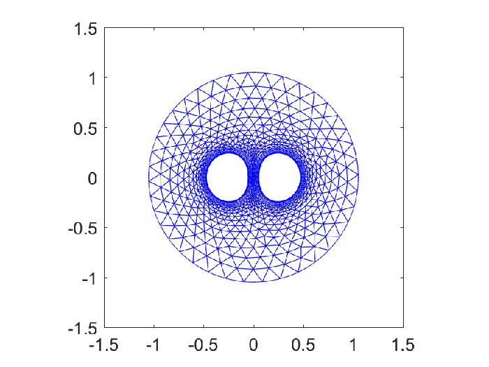
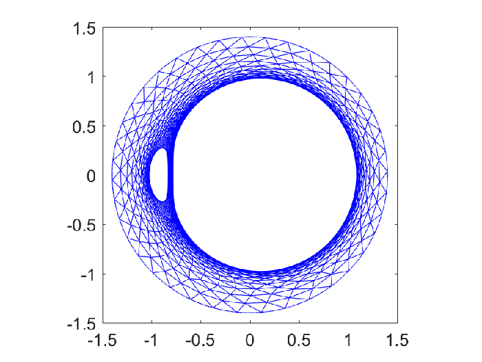
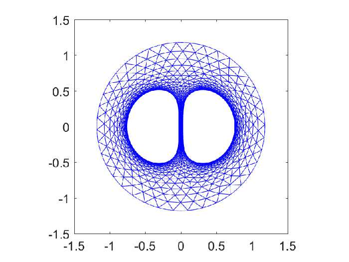
Starting from an initial small deformation which is close to axisymmetric, then we are typically led to an axisymmetric cavity solution as shown in Figure 10(a). On the other hand, if we start from an initial deformation which is not close to axisymmetric, then we are led to non-axisymmetric cavity solutions, in which either the left or the right cavity prevails (see Figure 10(b) and Figure 10(c)). It is worth mentioning here that our numerical solutions spontaneously realize the two energetically possible scenarios characterized by Henao & Serfaty in [12], where it is proved that, in incompressible nonlinear elasticity ( $s=n$ ) multi-cavity problems, when the distance between the initial defects are small compared with the radius of the grown cavity, either 1) cavities are pushed together to form one equivalent round cavity (as $\rho\rightarrow 0$ ); or 2) all but one cavity are of very small volume; while when the distance is much bigger, there is a third scenario: 3) the cavities prefer to be spherical in shape and well separated.

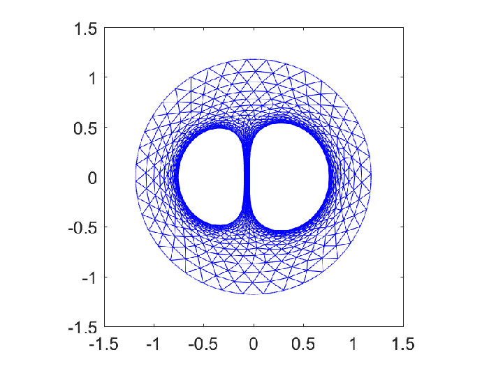
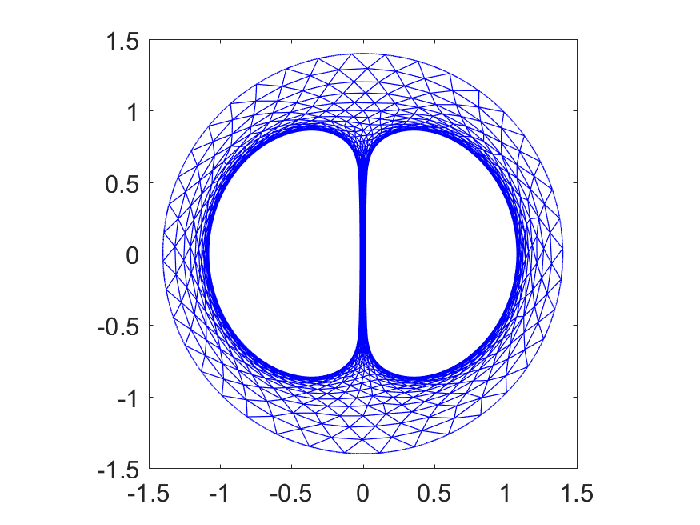
Our numerical experiments as well as the analytical results of Henao & Serfaty [12] suggest that, for a given multi-cavity problem, there should exist a critical $\lambda_{c}>1$ such that, as $\lambda$ decreases across $\lambda_{c}$ , the multi-cavity solutions will experience a change from the scenarios 1 or 2 or both to the scenario 3. Our numerical experiments actually captured the process of the change, of which some snapshots are shown in Figure 11 and Figure 12, where it is obviously seen that, for $\lambda\gg 1.18$ we have cavity solutions of both scenarios 1 and 2 (see Figures 11(a) and 12(a)), the difference of the two solutions narrows as $\lambda$ deceases across $1.18$ (see Figures 11(b) and 12(b)), and eventually become an indistinctive scenario 3 solution (compare Figures 11(c) and 12(c)).

Let $E_{s}$ and $E_{r}$ denote the elastic energy of the axisymmetric and right dominant numerical multi-cavity solutions respectively, Figure 13(a) shows $E_{s}-E_{r}$ as a function of $\lambda\in[1.0,1.4]$ , where we see that, for $\lambda<1.18$ , $E_{s}-E_{r}$ is essentially zero; while for $\lambda>1.18$ , $E_{s}-E_{r}$ grows fast. Let $v_{2}$ and $v_{1}$ denote the volumes of the right and left grown cavities of the multi-cavity solutions respectively. Our numerical experiments show that $v_{2}/v_{1}\approx 1$ for the axisymmetric numerical cavity solution for all $\lambda\in[1.0,1.4]$ , and for non-axisymmetric cavity solutions for all $\lambda\in[1.0,1.175]$ . Figure 13(b) shows that the volume ratio $v_{2}/v_{1}$ of the right dominant numerical cavity solution grows fast for $\lambda>1.18$ . Hence we are able to claim that the critical $\lambda_{c}\in(1.175,1.180)$ , and the greater volume ratio cavity solution is increasingly energetically favorable for $\lambda>\lambda_{c}$ .

6 Concluding remarks

The mixed finite element method introduced in this paper on multi-cavity growth problem in incompressible nonlinear elasticity is analytically proved to be locking-free and convergent, and numerically verified to be efficient. In fact, the method enables us to find a new bifurcation phenomenon in the multi-cavity growth problem.

It is of great interest to further study the bifurcation phenomena, including those found by Lian and Li in [7], and especially to explore their relationship with the material failure mechanism.

References

[1] Gent, A. N., Lindley, P. B., Internal rupture of bonded rubber cylinders in tension. Proc. R. Soc. London, A 249 (1958), 195-205.
[2] Zienkiewicz, O. C., Taylor. R.L., The finite element method : basic formulation and linear problems, vol. 1 (fourth edition). McGraw-Hill, London (1989).
[3] Su, C., Li, Z., A meshing strategy for a quadratic iso-parametric FEM in cavitation computation in nonlinear elasticity. J. Comp. Math. Appl., 330 (2018), 630-647.
[4] Su, C., Li, Z., Error analysis of a dual-parametric bi-quadratic FEM in cavitation computation in elasticity. SIAM J. Numer. Anal., 53(3) (2015), 1629-1649.
[5] Lian, Y., Li, Z., A dual-parametric finite element method for cavitation in nonlinear elasticity. J. Comput. Appl. Math., 236 (2011), 834-842.
[6] Lian, Y., Li, Z., A numerical study on cavitations in nonlinear elasticity-defects and configurational forces. Math. Models Meth. Appl. Sci., 21 (2011), 2551-2574.
[7] Lian, Y., Li, Z., Position and size effects on voids growth in nonlinear elasticity. Int. J. Fract., 173 (2012), 147-161.
[8] Huang, W., Li, Z., A Mixed Finite Element Method for Cavitation Computation in Incompressible Nonlinear Elasticity. arXiv:1710.04445v1.
[9] Brezzi, F., Fortion, M., Mixed and hybrid finite element methods. Springer-Verlag, New York (1991).
[10] Shi Z., Wang M., Finite element methods. Science Press, Beijing (2013).
[11] Henao, D., Mora, C. C., Fracture surfaces and the regular of inverses for BV deformations. Arch. Rat. Mech Anal., 201 (2011), 575-629.
[12] Henao, D., Serfaty, S., Energy estimates and cavity interaction for a critical-exponent cavitation model. Comm. Pure Appl. Math., 66(7), (2013), 1028-1101.
[13] Henao, D., Mora, C. C., Invertibility and weak continuity of the determinant for the modelling of cavitation and fracture in nonlinear elasticity. Arch. Rat. Mech. Anal., 197 (2010), 619-655.
[14] Megginson, R. E., An introduction to Banach space theory. Springer-Verlag, New York (1998).
[15] Dobrowolski, M., A mixed finite element method for approximating incompressible materials. SIAM J. Numer. Anal., 29 (1992), 365-389.
[16] Nirenberg, L., On elliptic partial differential equations. Ann. Scuola Norm. Sup. Pisa Sci. Fis. Mat. 13 (1959), 116-162.

	$\displaystyle\|\Pi_{1}\bm{v}\|^{2}_{1,2,\Omega_{\rho}}\lesssim$	$\displaystyle\|\bar{\Pi}_{1}\bm{v}\|^{2}_{1,2,\Omega_{\rho}}+\sum_{T}\|\bar{\Pi}_{2}(\bm{v}-\bar{\Pi}_{1}\bm{v})\|^{2}_{1,2,T}$
	$\displaystyle\lesssim$	$\displaystyle\|\bar{\Pi}_{1}\bm{v}\|^{2}_{1,2,\Omega_{\rho}}+\sum_{T}\dfrac{1}{\sigma^{4}}(h_{T}^{-2}\\|\bm{v}-\bar{\Pi}_{1}\bm{v}\\|^{2}_{0,2,T}+\|\bm{v}-\bar{\Pi}_{1}\bm{v}\|^{2}_{1,2,T})\lesssim\dfrac{1}{\sigma^{4}}\|\bm{v}\|_{1,2,\Omega_{\rho}}^{2}.$

		$\displaystyle\Big\|\int_{\Omega_{\rho}}(\|\nabla\bar{\bm{u}}\|^{s-2}-\|\nabla\bm{u}_{h}\|^{s-2})(\nabla\bm{u}_{h}:\nabla\bm{v}_{h})\,\mathrm{d}\bm{x}\Big\|$
	$\displaystyle=$	$\displaystyle\Big\|\int_{\Omega_{\rho}}(s-2)\|\nabla\bm{u}_{\eta}\|^{s-4}\big(\nabla\bm{u}_{\eta}:(\nabla\bar{\bm{u}}-\nabla\bm{u}_{h})\big)(\nabla\bm{u}_{h}:\nabla\bm{v}_{h})\,\mathrm{d}\bm{x}\Big\|$
	$\displaystyle\leq$	$\displaystyle c^{s-4}(s-2)\\|\nabla\bar{\bm{u}}-\nabla\bm{u}_{h}\\|_{0,2,\Omega_{\rho}}\\|\nabla\bm{v}_{h}\\|_{0,2,\Omega_{\rho}},$

A Mixed Finite Element Method for Multi-Cavity Computation in Incompressible Nonlinear ElasticityThanks: The research was supported by the NSFC projects 11171008 and 11571022.

Abstract

1 Introduction

2 The mixed finite element method

2.1 The iso-parametric P2+P_{2}^{+}-P1P_{1} element

Remark 1.

2.2 The iso-parametric Q2Q_{2}-P1P_{1} element

2.3 The partition of Ωρ\Omega_{\rho}

2.4 The discrete problem

Remark 2.

Remark 3.

3 Stability analysis of the method

Lemma 1.

Lemma 2.

Lemma 3.

Proof.

Therorem 1.

Proof.

4 Convergence analysis of the method

Lemma 4.

Lemma 5.

Proof.

Remark 4.

Therorem 2.

Proof.

Therorem 3.

Proof.

5 Numerical experiments and results

5.1 Single pre-existing defect case

5.2 Two pre-existing defects case

6 Concluding remarks

References

2.1 The iso-parametric $P_{2}^{+}$ - $P_{1}$ element

2.2 The iso-parametric $Q_{2}$ - $P_{1}$ element

2.3 The partition of $\Omega_{\rho}$