Explicit Constructions of MBR and MSR Codes
for Clustered Distributed Storage

This paper designs explicit coding schemes which achieve capacity $\mathcal{C}(\alpha,\beta_{I},\beta_{c})$ of clustered DSSs computed in [14]. Mainly, we focus on two types of exact-regenerating codes, the minimum-bandwidth-regenerating (MBR) code and the minimum-storage-regenerating (MSR) code, under the setting of maximal helper nodes. Both codes achieve capacity of clustered DSSs, while the former uses the minimum repair bandwidth and the latter assumes the minimum node storage overhead. The MBR codes suggested in this paper cover arbitrary system parameter values of $n,k,L,\beta_{I}$ and $\beta_{c}$, while different types of code constructions are proposed depending on $\epsilon=\beta_{c}/\beta_{I}$, the ratio of cross- to intra-cluster repair bandwidths. Moreover, when $\beta_{I}=\beta_{c}$, the suggested MBR code reduces to an existing MBR code in [4], i.e., the proposed scheme can be viewed as a generalization of the code construction in [4]. Regarding MSR codes, we consider two important scenarios of $\epsilon=0$ and $\epsilon\in[\frac{1}{n-k},1]$. The former represents the system where cross-cluster communication is not possible. The latter corresponds to the range of $\epsilon$ values that can achieve the minimum node storage overhead of $\alpha=\mathcal{M}/k$, where $\mathcal{M}=\mathcal{C}(\alpha,\beta_{I},\beta_{c})$ is the file size that we want to reliably store in a clustered DSS. When $\epsilon=0$, it is shown that appropriate application of locally repairable codes suggested in [18, 19] can be used as MSR codes for general $n,k,L$ settings with the application rule depending on the parameter setting. For the $\epsilon\in[\frac{1}{n-k},1]$ case, we first show that existing MSR codes for non-clustered DSSs, e.g., [6, 3], can be used as MSR codes for clustered DSSs with arbitrary $n,k,L$, when the repair rule is modified to adjust the given $\epsilon$ setting. Moreover, a simple MSR code with a small required field size is suggested for $L\geq 3$ under the conditions of $\epsilon=\frac{1}{n-k}$ and $n=kL$. The proposed MBR and MSR coding schemes can be implemented in wireless storage networks having a clustered topology or data centers with multiple racks, depending on the network bandwidth constraints and the node storage overhead constraints.

The MBR codes suggested in this paper for clustered DSSs are based on the MBR codes in [4, 5] for non-clustered DSSs with $\beta_{I}=\beta_{c}$. However, critical contributions are added in our code constructions: 1) we modify the existing works to reflect the clustered nature of distributed storage having $\beta_{I}\geq\beta_{c}$, 2) a novel mathematical analysis (which includes applying the majorization theory [20]) on the modified codes is developed to prove the exact regeneration property and the data reconstruction property for general $n,k,L,\epsilon$ settings. Here we note that the code proposed in the present paper can be viewed as a generalization of the MBR code in [4] for application to clustered DSSs; the code proposed in Section IV reduces to the code in [4] by setting $\beta_{I}=\beta_{c}$.

Considering an extreme network scenario when a failed node can contact only a limited number of survived nodes, i.e., $\beta_{c}=0$ in the present paper, the concept of locally repairable codes (LRCs) are considered in various papers [21, 18, 22, 23, 24, 25]. Some of these works were on codes with local regeneration, i.e., LRCs which minimize the bandwidth required in the local repair processes. Especially, within the class of codes with local regeneration, the authors of [22, 23] provided local MBR codes where each local code is an MBR, while the authors of [23, 24] considered local MSR codes. Here we note that the construction rule of local MBR codes in [23, 22] are similar to that of the code suggested in Section III of the present paper. However, the required field size is much less for the code in Section III compared to the existing local MBR codes. A detailed comparison is provided in Section III-D.

Regarding the clustered topology of storage nodes in multi-rack data centers, there have been some research [26, 13, 1, 27, 28, 12] on designing regenerating codes for DSSs with multiple clusters, but to a limited extent. The coding scheme suggested in [26] is well suited for multi-rack systems, but not proven to be an MBR or an MSR code. The authors of [13] focused on designing MSR codes under the assumption of maximum intra-cluster communication $\beta_{I}$. The focus is different from the present paper which designs MSR and MBR codes depending on given $\beta_{I}$ and $\beta_{c}$. The authors of [28] provided an explicit coding scheme which reduces the repair bandwidth of clustered DSSs under the condition that each failed node can be exactly regenerated by contacting any one of other clusters. The approach of [28] is different from that of the present paper in the sense that it does not consider the scenario with unequal intra- and cross-cluster repair bandwidths. Moreover, the coding scheme in [28] is shown to be a minimum-bandwidth-regenerating (MBR) code for some limited parameter setting, while the present paper proposes MBR codes for arbitrary parameters. An MSR code for clustered DSSs has been suggested in [12], but the data retrieval condition of [12] is different from that of the present paper. The authors of [12] considered the scenario where data can be collected by contacting arbitrary $k$ out of $n$ clusters, while data is retrieved by contacting any $k$ out of $n$ nodes in the present paper. Thus, the storage versus repair bandwidth tradeoff curves for the present paper and [12] are different. In short, the code in [12] and the code in the present paper achieve different tradeoff curves. Another recent work [27] suggested MSR codes for clustered DSS. On one hand, the authors of [27] assumed that intra-cluster repair bandwidth does not incur any cost, and only concerned with minimizing the amount of information transmitted across different clusters. On the other hand, the present paper considers both the intra- and cross-cluster repair burdens, and proposes MBR and MSR codes which minimize the overall repair burden for a given $\epsilon=\beta_{c}/\beta_{I}$, the ratio of cross- to intra-cluster repair bandwidth. Thus, the code in [27] and the code in this paper achieve different tradeoff curves. Compared to the conference version [1] of the current work, this paper adds an MSR code construction rule for $\epsilon\in[\frac{1}{n-k},1]$, and provides another MSR code for $\epsilon=\frac{1}{n-k},n=kL$ having a much smaller field size. Moreover, MBR codes for general $n,k,L,\epsilon$ setting are added in the present paper, which were not included in [1].

Here, we briefly summarize the clustered distributed storage system model, which is originally suggested in [11, 14]. The clustered model is motivated by the practical scenario where data centers consist of storage nodes dispersed into multiple racks, with the cross-rack bandwidth small compared to the intra-rack bandwidth [29]. However, the application is not limited to the multi-rack data centers; the clustered model can be naturally applied to general distributed storage systems (e.g. wireless sensor network) with clustered topology, where the amount of available cross-cluster bandwidth is different from that of the available intra-cluster bandwidth. Consider a file with $\mathcal{M}$ symbols to be stored. The file is encoded and distributed into $n$ storage nodes, which are uniformly dispersed into $L$ clusters. We use the notation $n_{I}=n/L$ to indicate the number of nodes in each cluster. Moreover, each node contains $\alpha$ symbols. Fig. 1a provides the system model when $n=12,L=3$.

Consider the scenario where a data collector wants to retrieve the original file. Assume that it contacts arbitrary $k<n$ nodes in the system, irrespective of the cluster which contains the node. Moreover, when a node fails, it is regenerated by contacting $n_{I}-1$ survived nodes in the same cluster and $n-n_{I}$ nodes in other clusters. This implies that the total number of helper nodes are $n-1$, i.e., the regeneration process utilizes the maximum number of helper nodes. According to Proposition 1 of [14], this maximum helper node setup is the capacity-maximizing choice. In the regeneration process, each node in the same cluster transmits $\beta_{I}$ symbols, while each node in other clusters sends $\beta_{c}$ symbols. Fig. 1b illustrates the regeneration process of a failed node. Recall that the clustered model considers practical scenarios with limited cross-cluster communication bandwidth, compared to the abundant intra-cluster communication bandwidth. Thus, we follow the assumption $\beta_{I}\geq\beta_{c}$ used in [14]. Moreover, we use the parameter $\epsilon=\beta_{c}/\beta_{I}$, which is defined in [14] and represents the ratio of the cross-cluster repair bandwidth to the intra-cluster repair bandwidth. It is easily seen that $0\leq\epsilon\leq 1$ holds. According to the regeneration process illustrated above, the repair bandwidth $\gamma$ is expressed as

In the clustered DSS with given parameters of $(n,k,L,\alpha,\beta_{I},\beta_{c})$, the authors of [14] defined capacity, the maximum amount of data that is reliably retrievable by contacting arbitrary $k$ nodes. The capacity expression for the clustered DSS is obtained in Theorem 1 of [14]:

where

We consider clustered distributed storage systems specified by parameters ($n,k,L,\alpha,\beta_{I},\beta_{c}$). Recall that the maximum file size that can be reliably stored in this system is capacity $\mathcal{C}(\alpha,\beta_{I},\beta_{c})$ in (2). For a given $\epsilon=\beta_{c}/\beta_{I}$, we denote the capacity as $\mathcal{C}(\alpha,\gamma)$ using two important system parameters: node storage capacity $\alpha$ and repair bandwidth $\gamma$ in (1). Consider the target of reliably storing a file with size $\mathcal{M}$. The feasible $(\alpha,\gamma)$ points which satisfy $\mathcal{C}(\alpha,\gamma)=\mathcal{M}$ are obtained in Corollary 1 of [14], and are illustrated in Fig. 2 which show a tradeoff relationship. In this figure, we focus on two important points $-$ MBR and MSR points $-$ which achieve capacity by using minimum system resources. Among the points having the minimum repair bandwidth $\gamma$, one with the smallest $\alpha$ is called the minimum-bandwidth-regenerating (MBR) point. The explicit regenerating coding schemes which achieve the MBR point is called MBR codes. Also, among the points with the minimum node capacity $\alpha$, one having the smallest $\gamma$ is called the minimum-storage-regenerating (MSR) point. The regenerating codes which achieve the MSR point is called the MSR codes. We denote the resource pair for an MBR code as $(\alpha,\gamma)=(\alpha_{\text{mbr}}^{(\epsilon)},\gamma_{\text{mbr}}^{(\epsilon)})$. Similarly, an MSR code has the resource pair $(\alpha,\gamma)=(\alpha_{\text{msr}}^{(\epsilon)},\gamma_{\text{msr}}^{(\epsilon)})$. Note that the explicit form of the resource pairs are given in Section II-C.

We aim at constructing MBR and MSR codes which achieve storage capacity $\mathcal{C}(\alpha,\gamma)=\mathcal{M}$. Under the clustered system model, the necessary and sufficient condition for a code being MBR (or MSR) is given as below. The validity of the suggested codes can be confirmed from Condition 1.

In the first part of this paper, we design explicit MBR codes for clustered distributed storage with arbitrary system parameters of $(n,k,L,\alpha,\beta_{I},\beta_{c})$. The explicit code construction depends on the $\epsilon=\beta_{c}/\beta_{I}$ ratio. In Section III, an MBR code is constructed when $\epsilon=0$, or equivalently $\beta_{c}=0$. Moreover, the MBR code construction for $0<\epsilon\leq 1$ (i.e., $\beta_{c}\neq 0$) is provided in Section IV. In the second part of this paper, we design MSR codes for clustered distributed storage. According to Theorem 3 of [14], node storage capacity of an MSR code satisfies

Recall that $\alpha=\mathcal{M}/k$ is the minimum storage overhead of each node in order to recover file size $\mathcal{M}$ by contacting $k$ nodes, as stated in [2]. Thus, the minimum node storage overhead $\alpha=\mathcal{M}/k$ is achievable only for $\epsilon\in[\frac{1}{n-k},1]$. Motivated by this fact, we focus on two cases: Section V provides the explicit MSR code construction when $\epsilon=0$, and MSR codes for the $\epsilon\in[\frac{1}{n-k},1]$ case is given in Section VI.

Here we recall explicit expressions for $(\alpha,\gamma)$ resource pairs of MBR and MSR codes for clustered distributed storage, which are stated in [14]. First, we define notations of

which represent the quotient and the remainder of $k/n_{I}$.

Note that the storage node capacity is equal to the repair bandwidth, i.e.,

for MBR codes with $0\leq\epsilon\leq 1$.

Throughout the paper, we use some useful additional notations. For a positive integer $n$, we denote $\{1,2,\cdots,n\}$ as $[n]$. For positive integers $a$ and $b$, we use the notation $a\mid b$ if $a$ divides $b$. Similarly, we write $a\nmid b$ if $a$ cannot divide $b$. Moreover, a clustered distributed storage system having parameters of $n,k,L$ is denoted as an $[n,k,L]-$clustered DSS. Note that this clustered system can be expressed as a two-dimensional representation, as in Fig. 3. In this structure, we denote the $j^{th}$ storage node in the $l^{th}$ cluster as $N{(l,j)}$. A vector is denoted as $\mathbf{v}$ using a bold-faced lower case letter. For positive integers $m$ and $n$, the set $\{y_{m},y_{m+1},\cdots,y_{n}\}$ is represented as $\{y_{i}\}_{i=m}^{n}$. The binomial coefficient $\frac{n!}{k!(n-k)!}$ is written as $\binom{n}{k}$.

Finally, we recall definitions on the locally repairable codes (LRCs) in [18, 19]. As defined in [19], an $(n,k,r)-$LRC represents a code of length $n$, which is encoded from $k$ information symbols. Every coded symbol of the $(n,k,r)-$LRC can be regenerated by accessing at most $r$ other symbols. As defined in [18], an $(n,r,d,\mathcal{M},\alpha)-$LRC takes a file of size $\mathcal{M}$ and encodes it into $n$ coded symbols, where each symbol is composed of $\alpha$ bits. Moreover, any coded symbol can be regenerated by contacting at most $r$ other symbols, and the code has the minimum distance of $d$.

Without a loss of generality, we set $\beta_{I}=1$. Then, from (12) and (1), the resource pair $(\alpha,\gamma)=(\alpha_{\text{mbr}}^{(0)},\gamma_{\text{mbr}}^{(0)})$ is given as

Moreover, combining (8) and (13), the maximum reliably storable file size $\mathcal{M}$ is expressed as

We now propose an explicit coding scheme with parameters $\alpha=\gamma=n_{I}-1,\beta_{I}=1,\beta_{c}=0$, satisfying the following:

• •

  A failed node is repaired within the cluster, by receiving $\beta_{I}=1$ symbol from each node in the same cluster.

• •

  Contacting any $k$ out of $n$ nodes can recover file size $\mathcal{M}$.

The suggested coding scheme is based on the repair-by-transfer (RBT) scheme devised in [4, 5]. Compared to these existing works on non-clustered (homogeneous) DSSs, the present paper applies the RBT scheme by reflecting the clustered nature of DSSs. Before specifying the code construction rule, we define a matrix $V_{t}$ as follows.

Note that Fig. 4 gives an example of graph $G_{t}$ and its incidence matrix $V_{t}$ for $t=4$. Using this definition, we provide an explicit code construction rule suitable for the $\epsilon=0$ case in Algorithm 1, under the setting of arbitrary $n,k,L$. For given $\mathcal{M}$ source symbols $\mathbf{s}=[s_{1},\cdots,s_{\mathcal{M}}]$, the algorithm specifies 1) the encoding rule and 2) the rule for distributing coded symbols to $n$ nodes $\{N(l,j)\}_{l\in[L],j\in[n_{I}]}$ in $L$ clusters.

The suggested coding scheme has the following properties, which are useful for proving Theorem 1.

Using this lemma, we show that Algorithm 1 provides a valid MBR code for any $n,k,L$ setting with $\epsilon=0$.

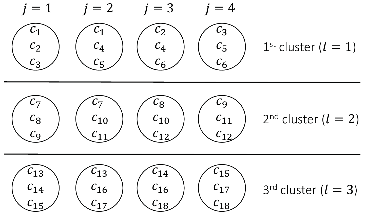
Consider a clustered distributed storage system with $n=12,k=6$ and $L=3$, as in Fig. 5. This implies $n_{I}=\frac{n}{L}=4,\theta=18$ and $\mathcal{M}=11$ from (14) and (16). Suppose the code in Algorithm 1 is applied to the system, for given $\mathcal{M}=11$ source symbols $\mathbf{s}=[s_{1},s_{2},\cdots,s_{11}]^{T}$. As a first step, $[\theta,\mathcal{M}]=[18,11]-$MDS code is applied for encoding, which results in $\theta=18$ coded symbols $\mathbf{c}=[c_{1},c_{2},\cdots,c_{18}]^{T}$. Next, the coded symbols are allocated into different nodes as follows: node $N(l,j)$ stores $c_{6(l-1)+i}$ if and only if $V_{4}(j,i)=1$. Here, the ranges of parameters are $l\in[3],j\in[4]$ and $i\in[6]$. Using matrix $V_{4}$ in Fig. 4, the coded symbols are distributed as in Fig. 5. Each circle represents a storage node, which stores $\alpha=3$ coded symbols. As an example of $(l,j)=(2,3)$, node $N{(2,3)}$ stores three coded symbols: $c_{8},c_{10}$ and $c_{12}$.

Exact Regeneration: Suppose node $N(2,3)$ fails. Then, node $N(2,1)$ gives $c_{8}$, node $N(2,2)$ gives $c_{10}$, and node $N(2,4)$ gives $c_{12}$. These three symbols are stored in the new storage node for replacing $N(2,3)$. This regeneration process satisfies $\beta_{I}=1$ and $\beta_{c}=0$. The same argument holds for arbitrary single-node failure events.

Data Reconstruction: Suppose that the data collector connects to $k=6$ nodes, say, $N(1,1)$, $N(1,2)$, $N(1,3)$, $N(1,4)$, $N(2,1),$ and $N(2,2)$. It is easy to see that this process allows the retrieval of the eleven coded symbols $\{c_{i}\}_{i=1}^{11}$. By using the MDS property of the $[\theta,\mathcal{M}]=[18,11]$ code used in Algorithm 1, we can easily obtain $\{s_{i}\}_{i=1}^{11}$ from the retrieved coded symbols $\{c_{i}\}_{i=1}^{11}$. The same can be shown for any arbitrary choice of $k=6$ nodes.

Recall that when $\epsilon=0$, no cross-cluster repair bandwidths are allowed. This scenario reminds one of a class of codes called locally repairable codes (LRCs) [18], which regenerate a failed node by contacting some limited number of nodes. There have been extensive works on LRCs, with some [22, 23] especially focusing on constructing LRCs with the MBR property. These codes are called local MBR codes. Here we compare our MBR code suggested in Algorithm 1 with the local MBR codes previously designed by other researchers. In Construction 6.3 of [23], the authors proposed a local MBR code based on the repair-by-transfer (RBT) scheme, similar to the code suggested in the current paper. However, the code in [23] requires a finite field with size $\binom{n\alpha/2}{\mathcal{M}}=\binom{n(n_{I}-1)/2}{\mathcal{M}}$, while the code in the current paper requires a much smaller field size of $\theta=\binom{n_{I}}{2}L=n(n_{I}-1)/2$, when RS code is used for $[\theta,\mathcal{M}]-$MDS encoding. In addition, the local MBR code suggested in Construction II.1 of [22] requires a finite field with size much larger than that of the MBR code suggested in the current paper. To be specific, the required field size of the code in [22] is $q^{m}$ for some prime number $q\geq 2$ and $m\geq LK_{\text{local}}$, where $K_{\text{local}}$ is the scalar dimension of a local code satisfying $K_{\text{local}}=\alpha(n_{I}-1)-\binom{n_{I}-1}{2}\geq\frac{(n_{I}-1)^{2}}{2}\simeq\frac{n_{I}(n_{I}-1)}{2}$ . Thus, one gets $q^{m}\geq q^{LK_{\text{local}}}\simeq q^{\theta}$, which is far greater than $\theta$, the field size of our MBR code.

For a given $0<\epsilon\leq 1$, we consider MBR codes with resource pair $(\alpha,\gamma)=(\alpha_{\text{mbr}}^{(\epsilon)},\gamma_{\text{mbr}}^{(\epsilon)})$, which reliably store file size $\mathcal{M}=\mathcal{C}(\alpha,\gamma)$. Let us assume that $\chi\coloneqq 1/\epsilon=\beta_{I}/\beta_{c}$ is a positive integer. Without losing generality, we set $\beta_{I}=\chi$ and $\beta_{c}=1$. From (12) and (1), we have

Under this setting, the following proposition provides a simplified form of the capacity expression.

In Algorithm 2, we propose an MBR code for $0<\epsilon\leq 1$. In the symbol allocation rule in Step 2 of Algorithm 2, coded symbols are classified as global symbols and local symbols. Note that global symbols are shared either among nodes in the same cluster or among nodes in other clusters, while local symbols are shared among nodes in the same cluster only. An example of code construction in Fig. 6 with an explanation in Section IV-C provides an insight on global/local symbols. Now we provide properties of the code in Algorithm 2, which are useful for proving Theorem 2.

Based on this Lemma, the code in Algorithm 2 is shown to be an MBR code for any $n,k,L$ setting with $0<\epsilon\leq 1$, as stated in the following Theorem.

Consider the scenario where $n=6,k=3,L=2,\beta_{I}=3$ and $\beta_{c}=1$ (i.e., $\chi=3$ or $\epsilon=1/3$), as in Fig. 6. This implies $n_{I}=n/L=3$ and $\alpha=(n_{I}-1)\chi+(n-n_{I})=9$. Moreover, $\mathcal{M}=18$ and $\theta=27$ from (18), (19). First, we apply a $[\theta,\mathcal{M}]=[27,18]-$MDS code to the original source symbol $\bm{s}=[s_{1},s_{2},\cdots,s_{18}]^{T}$, which results in $\bm{c}=[c_{1},c_{2},\cdots,c_{27}]^{T}$. Then, the coded symbols are distributed as follows: node $N(l,j)$ stores

• •

  $c_{i_{1}}$ if and only if $V_{6}(3(l-1)+j,i_{1})=1$.

• •

  $c_{15+3(2l+t-3)+i_{2}}$ if and only if $V_{3}(j,i_{2})=1$, for $t=1,2$

Here, $l\in[2],j\in[3],i_{1}\in[15],i_{2}\in[3]$. Using the following $V_{6}$ and $V_{3}$ matrices,

the coded symbols are distributed as in Fig. 6. Each rectangle represents a storage node, which stores $\alpha=9$ coded symbols. The numbers in a rectangle represent the indices of the coded symbols contained in the node. For example, when $(l,j)=(1,2)$, node $N(l,j)=N(1,2)$ stores $\{c_{i}\}$ for $i=1,6,7,8,9,16,18,19$, and $21$. Here, note that each of the $\{c_{i}\}_{i=1}^{15}$ global symbols is shared either among the nodes within the same cluster or among the nodes in different clusters. Moreover, $\{c_{i}\}_{i=16}^{27}$ are local symbols: $\{c_{i}\}_{i=16}^{21}$ are shared among the nodes in the $1^{st}$ cluster only, while $\{c_{i}\}_{i=22}^{27}$ are shared among the nodes in the $2^{nd}$ cluster only.

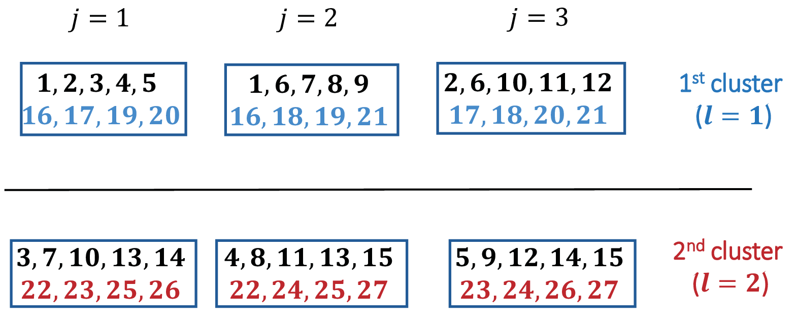
Exact Regeneration: Suppose node $N(1,2)$ is broken. Then, $N(1,1)$ provides $c_{1},c_{16},c_{19}$, while $N(1,3)$ gives $c_{6},c_{18},c_{21}$. The nodes $N(2,1),N(2,2),N(2,3)$ transmit $c_{7},c_{8},c_{9}$, respectively. This completely regenerates the failed node $N(1,2)$. Any single node failure can be repaired in a similar way.

Data Reconstruction: Consider an arbitrary contact of $k=3$ nodes, say, three nodes in the $1^{st}$ cluster in Fig. 6. Note that this contact can retrieve $18$ coded symbols $c_{i}$ for $i\in\{1,2,\cdots,12\}\cup\{16,17,\cdots,21\}$. By using the MDS property of the $[\theta,\mathcal{M}]=[27,18]$ code used in Algorithm 2, we obtain $\{s_{i}\}_{i=1}^{18}$ from the retrieved $18$ coded symbols. The same can be shown for any arbitrary contact of $k=3$ nodes.

We consider the MSR point $(\alpha,\gamma)=(\alpha_{\text{msr}}^{(\epsilon)},\gamma_{\text{msr}}^{(\epsilon)})$ which can reliably store $\mathcal{M}=\mathcal{C}(\alpha,\gamma)$. The following property specifies the system parameters for the $\epsilon=0$ case.

We now examine how to construct an MSR code when $n_{I}$ divides $k$, i.e., $n_{I}\mid k$ holds. The following theorem shows that a locally repairable code constructed in [18] with locality $r=n_{I}-1$ is a valid MSR code for $n_{I}\mid k$.

Fig. 7 illustrates an example of the MSR code for the $\epsilon=0$ and $n_{I}\mid k$ case, which is constructed using the LRC in [18]. In the $[n,k,L]=[6,3,2]-$clustered DSS scenario, the parameters are set to

Thus, each storage node contains $\alpha=3$ symbols, while the $[n,k,L]$ clustered DSS aims to reliably store a file of size $\mathcal{M}=6$. This code has two properties, 1) exact regeneration and 2) data reconstruction:

1. 1.

   Any failed node can be exactly regenerated by contacting $n_{I}-1=2$ nodes in the same cluster,

2. 2.

   Contacting any $k=3$ nodes can recover the original file $\{x_{i}^{(j)}:i\in[3],j\in[2]\}$ of size $\mathcal{M}=6$.

The first property is obtained from the fact that $y_{i}^{(1)},y_{i}^{(2)}$ and $s_{i}=y_{i}^{(1)}+y_{i}^{(2)}$ form a $(3,2)$ MDS code for $i\in[6]$. The second property is obtained as follows. For contacting arbitrary $k=3$ nodes, three distinct coded symbols $\{y_{i_{1}}^{(1)},y_{i_{2}}^{(1)},y_{i_{3}}^{(1)}\}$ having superscript one and three distinct coded symbols $\{y_{j_{1}}^{(2)},y_{j_{2}}^{(2)},y_{j_{3}}^{(2)}\}$ having superscript two can be obtained for some $i_{1},i_{2},i_{3}\in[6]$ and $j_{1},j_{2},j_{3}\in[6]$. From Fig. 7a, the information $\{y_{i_{1}}^{(1)},y_{i_{2}}^{(1)},y_{i_{3}}^{(1)}\}$ suffice to recover $x_{1}^{(1)},x_{2}^{(1)},x_{3}^{(1)}$. Similarly, the information $\{y_{j_{1}}^{(2)},y_{j_{2}}^{(2)},y_{j_{3}}^{(2)}\}$ suffice to recover $x_{1}^{(2)},x_{2}^{(2)},x_{3}^{(2)}$. This completes the proof for the second property. Note that this coding scheme is already suggested by the authors of [18], while the present paper proves that this code also achieves the MSR point of the $[n,k,L]-$clustered DSS, in the case of $\epsilon=0$ and $n_{I}\mid k$.

Here we construct an MSR code when the given system parameters satisfy $n_{I}\nmid k$. The theorem below shows that the optimal $(n,k-q,n_{I}-1)-$LRC designed in [19] is a valid MSR code when $n_{I}\nmid k$ holds.

Fig. 8 illustrates an example code construction for the $n_{I}\nmid k$ case. Without losing generality, we consider the $\alpha=1$ case; applying this code for $\alpha$ times in a parallel manner achieves the MSR point for the general case with arbitrary positive integer $\alpha$. In the $[n=6,k=4,L=2]$ clustered DSS with $\epsilon=0$, system parameters are

References

- [1] J.-y. Sohn, B. Choi, and J. Moon, “A class of MSR codes for clustered distributed storage,” in 2018 IEEE International Symposium on Information Theory (ISIT). IEEE, 2018, pp. 2366–2370.
- [2] A. G. Dimakis, P. B. Godfrey, Y. Wu, M. J. Wainwright, and K. Ramchandran, “Network coding for distributed storage systems,” IEEE Transactions on Information Theory, vol. 56, no. 9, pp. 4539–4551, 2010.
- [3] K. V. Rashmi, N. B. Shah, and P. V. Kumar, “Optimal exact-regenerating codes for distributed storage at the msr and mbr points via a product-matrix construction,” IEEE Transactions on Information Theory, vol. 57, no. 8, pp. 5227–5239, 2011.
- [4] K. Rashmi, N. B. Shah, P. V. Kumar, and K. Ramchandran, “Explicit construction of optimal exact regenerating codes for distributed storage,” in Communication, Control, and Computing, 2009. Allerton 2009. 47th Annual Allerton Conference on. IEEE, 2009, pp. 1243–1249.
- [5] N. B. Shah, K. V. Rashmi, P. V. Kumar, and K. Ramchandran, “Distributed storage codes with repair-by-transfer and nonachievability of interior points on the storage-bandwidth tradeoff,” IEEE Transactions on Information Theory, vol. 58, no. 3, pp. 1837–1852, 2012.
- [6] C. Suh and K. Ramchandran, “Exact-repair MDS code construction using interference alignment,” IEEE Transactions on Information Theory, vol. 57, no. 3, pp. 1425–1442, 2011.
- [7] V. R. Cadambe, S. A. Jafar, H. Maleki, K. Ramchandran, and C. Suh, “Asymptotic interference alignment for optimal repair of mds codes in distributed storage,” IEEE Transactions on Information Theory, vol. 59, no. 5, pp. 2974–2987, 2013.
- [8] T. Ernvall, “Codes between MBR and MSR points with exact repair property,” IEEE Transactions on Information Theory, vol. 60, no. 11, pp. 6993–7005, 2014.
- [9] S. Goparaju, A. Fazeli, and A. Vardy, “Minimum storage regenerating codes for all parameters,” IEEE Transactions on Information Theory, vol. 63, no. 10, pp. 6318–6328, Oct 2017.
- [10] M. Ye and A. Barg, “Explicit constructions of high-rate MDS array codes with optimal repair bandwidth.” IEEE Trans. Information Theory, vol. 63, no. 4, pp. 2001–2014, 2017.
- [11] J. y. Sohn, B. Choi, S. W. Yoon, and J. Moon, “Capacity of clustered distributed storage,” in 2017 IEEE International Conference on Communications (ICC), May 2017.
- [12] N. Prakash, V. Abdrashitov, and M. Médard, “The storage vs repair-bandwidth trade-off for clustered storage systems,” arXiv preprint arXiv:1701.04909, 2017.
- [13] Y. Hu, X. Li, M. Zhang, P. P. Lee, X. Zhang, P. Zhou, and D. Feng, “Optimal repair layering for erasure-coded data centers: From theory to practice,” arXiv preprint arXiv:1704.03696, 2017.
- [14] J.-y. Sohn, B. Choi, S. W. Yoon, and J. Moon, “Capacity of clustered distributed storage,” IEEE Transactions on Information Theory, vol. 65, no. 1, pp. 81–107, 2019.
- [15] N. Prakash, V. Abdrashitov, and M. Médard, “The storage vs repair-bandwidth trade-off for clustered storage systems,” IEEE Transactions on Information Theory, pp. 1–1, 2018.
- [16] B. Choi, J.-y. Sohn, S. W. Yoon, and J. Moon, “Secure clustered distributed storage against eavesdroppers,” in 2017 IEEE International Conference on Communications (ICC). IEEE, 2017, pp. 1–6.
- [17] ——, “Secure clustered distributed storage against eavesdropping,” IEEE Transactions on Information Theory, 2019.
- [18] D. S. Papailiopoulos and A. G. Dimakis, “Locally repairable codes,” IEEE Transactions on Information Theory, vol. 60, no. 10, pp. 5843–5855, 2014.
- [19] I. Tamo, D. S. Papailiopoulos, and A. G. Dimakis, “Optimal locally repairable codes and connections to matroid theory,” IEEE Transactions on Information Theory, vol. 62, no. 12, pp. 6661–6671, 2016.
- [20] P. Vaidyanathan, S.-M. Phoong, and Y.-P. Lin, Signal processing and optimization for transceiver systems. Cambridge University Press, 2010.
- [21] P. Gopalan, C. Huang, H. Simitci, and S. Yekhanin, “On the locality of codeword symbols,” IEEE Transactions on Information Theory, vol. 58, no. 11, pp. 6925–6934, 2012.
- [22] G. M. Kamath, N. Silberstein, N. Prakash, A. S. Rawat, V. Lalitha, O. O. Koyluoglu, P. V. Kumar, and S. Vishwanath, “Explicit MBR all-symbol locality codes,” in 2013 IEEE International Symposium on Information Theory, July 2013, pp. 504–508.
- [23] G. M. Kamath, N. Prakash, V. Lalitha, and P. V. Kumar, “Codes with local regeneration and erasure correction,” IEEE Transactions on Information Theory, vol. 60, no. 8, pp. 4637–4660, Aug 2014.
- [24] A. S. Rawat, O. O. Koyluoglu, N. Silberstein, and S. Vishwanath, “Optimal locally repairable and secure codes for distributed storage systems,” IEEE Transactions on Information Theory, vol. 60, no. 1, pp. 212–236, 2014.
- [25] N. Silberstein, T. Etzion, and M. Schwartz, “Locality and availability of array codes constructed from subspaces,” IEEE Transactions on Information Theory, 2018.
- [26] M. A. Tebbi, T. H. Chan, and C. W. Sung, “A code design framework for multi-rack distributed storage,” in Information Theory Workshop (ITW), 2014 IEEE. IEEE, 2014, pp. 55–59.
- [27] Z. Chen and A. Barg, “Explicit constructions of MSR codes for clustered distributed storage: The rack-aware storage model,” arXiv preprint arXiv:1901.04419, 2019.
- [28] S. Sahraei and M. Gastpar, “Increasing availability in distributed storage systems via clustering,” arXiv preprint arXiv:1710.02653, 2017.
- [29] F. Ahmad, S. T. Chakradhar, A. Raghunathan, and T. Vijaykumar, “Shufflewatcher: Shuffle-aware scheduling in multi-tenant mapreduce clusters,” in 2014 USENIX Annual Technical Conference (USENIX ATC 14), 2014, pp. 1–13.