The Radial Acceleration Relation and a Magnetostatic Analogy in Quasilinear MOND
Abstract
Recently a remarkable relation has been demonstrated between the observed radial acceleration in disk galaxies and the acceleration predicted on the basis of baryonic matter alone. Here we study this relation within the framework of the modified gravity model MOND. The field equations of MOND automatically imply the radial acceleration relation for spherically symmetric galaxies, but for disk galaxies deviations from the relation are expected. Here we investigate whether these deviations are of sufficient magnitude to bring MOND into conflict with the observed relation. In the quasilinear formulation of MOND, to calculate the gravitational field of a given distribution of matter, an intermediate step is to calculate the “pristine field”, which is a simple nonlinear function of the Newtonian field corresponding to the same distribution of matter. Hence, to the extent that the quasilinear gravitational field is approximately equal to the pristine field, the radial acceleration relation will be satisfied. We show that the difference between the quasilinear and pristine fields obeys the equations of magnetostatics; the curl of the pristine field serves as the source for the difference in the two fields, much as currents serve as sources for the magnetic field. Using the magnetostatic analogy we numerically study the difference between the pristine and quasilinear fields for simple model galaxies with a Gaussian profile. Our principal finding is that the difference between the fields is small compared to the observational uncertainties and that quasilinear MOND is therefore compatible with the observed radial acceleration relation.
I Introduction
The problem of dark matter is one of the central problems in modern cosmology [1]. According to the conventional CDM paradigm, matter constitutes less than a third of the total energy density of the Universe. The bulk of this matter is non-baryonic. Many lines of evidence point to the existence of dark matter, notably the cosmic microwave background anisotropies [2] and observations of lensing [3], but dark matter has eluded direct detection [4] and its nature remains a mystery.
Rotation curves of disk galaxies provided the earliest compelling evidence for dark matter [5]. The observation that the rotation velocity generically approaches a plateau instead of vanishing asymptotically is conventionally interpreted as evidence for a spherical dark matter halo that dominates the visible baryonic matter in the disk. Puzzling from this perspective were empirical observations such as the baryonic Tully-Fisher relation [6] that appear to suggest a strong connection between the rotation curves and the distribution of baryonic matter.
In an important recent study McGaugh et al. [7, 8] demonstrated a relation between the observed radial acceleration in disk galaxies and the acceleration predicted on the basis of baryonic matter alone. This empirical relation, dubbed the “radial acceleration relation” (RAR) is based on an impressive body of data, the SPARC dataset that represents near infrared observations by the Spitzer Space Telescope and 21 cm observations by radio astronomers over several decades [9]. The radial acceleration relation has to be explained by any tenable model of dark matter. There have already been several efforts to show that this relation is compatible with CDM cosmology[10, 11, 12]. There have also been efforts to understand this relationship using modified theories of gravity ranging from scalar tensor theories [13] to emergent gravity models [14, 15].
The modified gravity theory MOND was originally introduced [16] to account for galaxy rotation and it has had some phenomenological success, e.g., providing an explanation for the baryonic Tully-Fisher relation. However MOND and its relativistic completions have well-known problems on cluster and cosmological scales [17, 18, 19]. It is sometimes assumed that MOND predicts the observed radial acceleration relation, but in fact the MOND field equations imply such a relationship only for spherically-symmetric galaxies [20]. For disk galaxies deviations are to be expected. With the empirical discovery of the remarkable radial acceleration relation it becomes imperative to determine the magnitude of these deviations; that is the object of this paper. Our principle finding is that the deviations are small compared to the experimental uncertainties and that the MOND field equations are in fact compatible with the observed radial acceleration relation.
Our analysis is carried out in the framework of ‘quasilinear’ MOND [21]. Notwithstanding the name, quasilinear MOND is a highly nonlinear theory. In order to calculate the quasilinear gravitational field, , corresponding to a distribution of matter , an intermediate step is to calculate a “pristine field”, . The pristine field is related to the Newtonian field through a simple, nonlinear ‘interpolating function’, thus, if one was to plot observed versus Newtonian accelerations within pristine MOND, finding agreement with the radial acceleration relation would simply be a matter of choosing the right interpolating function [8]. To the extent that the quasilinear field is approximately equal to the pristine field, it will obey the radial acceleration relation. In order to demonstrate the approximate equality of the two fields we show that the difference obeys the equations of magnetostatics with analogous to the magnetic field and analogous to the current that sources . This analogy provides useful qualitative insights into the deviation field as well as a practical numerical scheme for its calculation.
Although the main focus of this paper is on modified gravity formulations of MOND it is worth noting that there is another class of models called modified inertia formulations of MOND. Although modified inertia models have received comparatively less attention [22], there has been an attempt to construct a relativistic formulation [23] and an interesting experimental test has been proposed [24]. It would be desirable in future work to explore possible contrasts between the predictions of modified inertia and modified gravity theories of MOND for galactic motion along the lines suggested by [22].
For simplicity we study simple model galaxies with a Gaussian profile. Our methods as well as our results will easily carry over to other more realistic galaxy models. The numerical analysis is most efficiently done by use of the fast Fourier transform although there are some subtleties that arise due to the long range nature of gravitational forces. Key results are presented in fig 2 which shows that the current distribution for a disk galaxy resembles a Helmholtz gradient coil; fig 4 in which the dependence of the deviation on distance from the galactic center and on the aspect ratio of the disk galaxy is systematically investigated; and fig 5 in which we display the computed radial acceleration relation for our model galaxies. Comparison of this plot with the observed radial acceleration relation leads to our conclusion.
II Magnetostatic analogy for MOND gravity
II.1 Quasilinear MOND
In Newtonian gravity, the acceleration due to gravity obeys the field equations
| (1) |
Here is the mass distribution producing the gravitational field. In the pristine formulation of MOND [16] a test particle however experiences an acceleration which is related to the Newtonian acceleration via the algebraic relation
| (2) |
Here m/s2 is the MOND acceleration scale and the interpolating function has the asymptotic behavior for and for . Thus the observed acceleration of the test particle matches the Newtonian prediction when the Newtonian gravitational field is strong but is significantly enhanced when the Newtonian field is weak on the MOND scale. Pristine MOND exactly reproduces the radial acceleration relation; indeed the observed radial acceleration relation may be regarded as a measurement of the MOND acceleration and the interpolating function .
However, pristine MOND suffers from physical inconsistencies and lacks a Lagrangian formulation. Thus it cannot be considered a viable alternative theory of gravitation as noted in [21] and [25]. These authors introduced nonlinear MOND [25] and quasilinear MOND [21] as viable alternatives to Newtonian gravity; in this paper we focus on quasilinear MOND. Within quasilinear MOND the acceleration of the test particle is not equal to the pristine field but to the quasilinear field which is determined by solving
| (3) |
Invoking the Helmholtz decomposition of vector fields we see that is the curl free part of . The divergence of (or more precisely ) has the interpretation of being the combined density of dark and baryonic matter that would be required to produce the same observed acceleration of the test mass if Newtonian gravity prevailed.
To complete the formulation of quasilinear MOND we must specify the interpolating function . A simple form that has the desired asymptotic behavior is
| (4) |
An alternative form, following ref [7], is to take
| (5) |
II.2 Magnetostatic Analogy
For a spherically symmetric galaxy is curl free and hence . In this case it automatically follows that the observed acceleration will be a simple function of the Newtonian gravitational field produced by the baryonic matter in the galaxy, namely, . However only in cases of exceptional symmetry will be curl free. Generically is not equal to and hence is not a local function of . For the radial acceleration relation to hold in quasilinear MOND we need at least in the galactic plane.
Whether the approximate equality holds for disc galaxies is the key question that is studied in this paper. In [20] the corresponding problem was pointed out for nonlinear MOND and an estimate was made of the size of the discrepancy between the observed acceleration and the pristine field strength in that theory. The new high quality data establishing the radial acceleration relation provides the impetus for the detailed study of quasilinear MOND reported in this paper.
To this end it is convenient to define
| (6) |
and
| (7) |
It then follows from eq (3) that
| (8) |
These are precisely the equations of magnetostatics. We have already noted that may be interpreted as the equivalent density of dark matter needed to reproduce MOND behavior within Newtonian gravity. Eq (8) reveals that may be interpreted as a current that sources the difference between and .
Given eq (8) provides an efficient way to calculate and thereby as we will discuss below. Formally one can write down a solution to eq (8) expressing in terms of using the Biot-Savart law. Whereas the relation eq (2) is local in the sense that at a given point is determined by at the same point, in sharp contrast the relation between and is not local. This shows that in general is not a local function of in quasilinear MOND.
III Simulated Radial Acceleration Relations for Model Galaxies
III.1 Model and Methods
We now introduce a simple model which allows us to study the deviation from the radial acceleration relation in disk galaxies. We take the galaxies to have a Gaussian profile
| (9) |
Here is the mass of the galaxy and is its radius. is a dimensionless parameter that characterizes the aspect ratio of the galaxy; corresponds to a spherically symmetric galaxy and to a flat disk. The characteristic radial acceleration scale within Newtonian gravity for this circumstance is . The MOND field of the galaxy is therefore fully determined by the dimensionless parameters and . We will work in a system of units wherein and . Then the parameter corresponds to a measure of the mass of the galaxy in our system of units. Other simple models used to describe disk galaxies [26] can be treated using our methods and will lead to similar results; the advantage of using the Gaussian model is that it allows us to do higher resolution numerics and to rapidly explore a broader range of MOND parameters. Hence we focus on the Gaussian model here.
The first step in our analysis is to calculate , the Newtonian field of the galaxy. Note that it is sufficient to calculate for since by linearity . Eq (1) has the simple solution
| (10) |
in Fourier space. (A tilde above a symbol denotes the Fourier transform.) The Newtonian field can therefore be efficiently calculated using the fast Fourier transform. We assume that the galaxy is located at the center of a cube of side and we sample functions at points on a regular cubic lattice with points per edge of the cube.
An amusing subtlety arises because of the long-range nature of the gravitational force. By using the Fourier transform we enforce a periodicity in the mass distribution and the gravitational field whereas in the real problem we wish to impose the boundary condition that the gravitational field vanishes far away from the galaxy. Naively one might suppose that in the limit that is sufficiently large the results would be insensitive to boundary conditions but it is easy to demonstrate that in fact a sensitivity to boundary conditions persists in the limit because of the inverse square falloff of the gravitational field [27]. The remedy is to calculate not the gravitational field of the disk galaxy directly but rather of the mass distribution . Here is a spherically symmetric distribution with a total mass, , the same as the galaxy distribution . The advantage is that the gravitational field of the difference falls off like a quadrupole as . This is a sufficiently rapid falloff that the result is insensitive to boundary conditions for sufficiently large . We can then construct the gravitational field corresponding to the galaxy distribution by adding the field corresponding to the spherical distribution which can be obtained analytically. In practice we take to be an isotropic Gaussian with radius .
Calculation of via eq (3) is now a simple matter of applying an algebraic function to . can be calculated by solving eq (8) by Fourier methods. In order to calculate the curl of it is helpful to first subtract a suitable isotropic function to ensure that the results are insensitive to boundary conditions much as we do in our computation of . In practice we subtract the pristine field corresponding to the isotropic distribution to facilitate the computations. Once and are determined it is a simple matter to obtain using eq (6).
In the results presented here we consider aspect ratios in the range and the mass parameter in the range . Over this range of parameters it is sufficient to calculate the Newtonian field using and . Smaller values of are more realistic for disk galaxies but would necessitate a finer grid. However in order to show the qualitative difference between pristine and quasilinear MOND, and to show that quasilinear MOND reproduces the observed radial acceleration relation it is sufficient to consider as discussed further in section III.2; we have verified that the results extrapolate smoothly with down to . The results are also insensitive to variations the size of the box and to the fineness of the discretization. We have also checked the accuracy of the calculated Newtonian field by using the multipole expansion to calculate the large distance asymptotic Newtonian field corresponding to the density profile eq (9). To check the accuracy of the calculated Newtonian field at short distances we have performed a non-trivial check described in appendix A. The subsequent calculation of is limited only by numerical roundoff since it only involves solving an algebraic relation. The calculation of from is similar to the calculation of and can be checked in similar ways.
III.2 Results
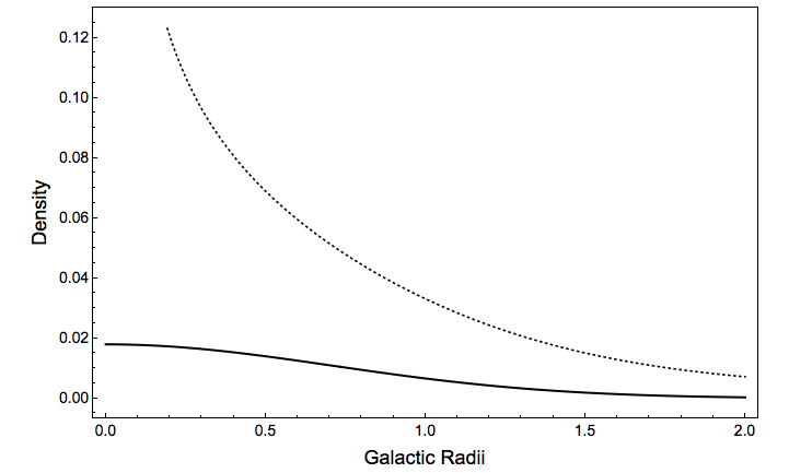
We start with a discussion of the quantity introduced in eq (3). If we cast a dark matter interpretation upon MOND we may regard as the density of baryonic matter and as the combined density of baryonic and dark matter. Fig 1 shows the two densities for an isotropic galaxy with aspect ratio and mass parameter . The plot of in the left panel corresponds to the Gaussian profile eq (9). The plot of in the right panel shows three interesting features. First the density is much greater than , consistent with the preponderance of dark matter compared to baryonic matter in the conventional CDM paradigm. Second the density extends to a greater distance from the galactic center much like a dark matter halo in the conventional CDM picture. Third the density has a weak divergence near the center of the galaxy ( for ); this is a generic feature of quasilinear MOND and it should be noted that it does not imply that the core of the galaxy has an infinite mass since the divergence is integrable. The plots in fig 1 were generated using analytic expressions for and which are available in the isotropic case. Our numerical methods can be employed to examine the behavior of for disk galaxies. Those results are of interest but they will be reported elsewhere [28] since they are tangential to the present study.
According to the magnetostatic analogy, the quantity may be regarded as a current that serves as the source for , the difference between the pristine and quasilinear MOND fields. Using the product rule it is easy to see that . Due to the azimuthal symmetry of the galaxy it is easy to see that neither nor can have an azimuthal component; it follows that must be purely azimuthal. Thus symmetry requires that the current that sources circulates about the axis of the galaxy. Similarly the assumed reflection symmetry of the galaxy about the - plane implies that the current must be antisymmetric under reflection about the - plane. Thus the currents circulate in opposite senses above and below the galactic plane. This is as far as symmetry arguments go. Fig 2 shows an explicit numerical calculation of the component of the current as a function of position in the - plane for a galaxy with aspect ratio and mass parameter . The plot shows two sharp peaks and two sharp anti-peaks that are related by the azimuthal and reflection symmetries noted above. It follows that the current is concentrated into two counter-propagating circular coils that are parallel to the - plane, one located above the plane and the other below it, analogous to a Helmholtz gradient coil. We can easily draw upon electromagnetic intuition to draw the lines of or to recognize that at large distance the resulting field will be quadrupolar.

We turn now to a comparison of the Newtonian, pristine MOND and quasilinear MOND gravitational fields. The upper panels of Fig.3 plot the radial component of the field as a function of the cylindrical coordinate . Each field is computed at 36 points in the galactic plane at distances that vary uniformly from zero to two galactic radii. Both plots are for galaxies with aspect ratio . The plot at left is for a galaxy that is deep in the MOND regime with parameter ; the plot on the right is deep in the Newtonian regime with parameter As expected the Newtonian field shown in blue vanishes both as and . We can check the large behavior using a multipole expansion and we can also perform a non-trivial check at small as described in Appendix A. The orange curves correspond to the pristine MOND acceleration. This is simply related to the Newtonian field via the algebraic function eq (2). The plots show that for small the pristine field is considerably enhanced relative to the Newtonian field but for large it is essentially equal to the Newtonian field. In fig 3 we have used the interpolating function in eq (4) but we have explicitly verified that the alternative interpolation eq (5) gives similar results. The black dashed curves show the radial component of the quasilinear acceleration. For this aspect ratio it appears that there is very little difference between the pristine and quasilinear fields at least in the galactic plane. We will examine this difference more closely below. The lower two panels of Fig.3 show the component of the Newtonian, pristine, and quasilinear fields as a function of . A key difference from the radial plots is that in this case the magnitude of the pristine acceleration is bigger than the magnitude of the quasilinear acceleration. This difference can be understood by picturing the difference between the two fields, , as the magnetic field of a Helmholtz gradient coil. Another noteworthy feature is that the difference between the pristine and quasilinear fields is bigger along the axis than in the galactic plane, though in neither case is the difference especially large.
Fig 4 shows the radial component of the difference between the pristine and quasilinear fields plotted as a function of . The plots are for a galaxy with mass parameter . Because the difference of the pristine and quasilinear fields is a small quantity the finiteness of the grid is visible in the jagged appearance of the plots; the deviations from a smooth fit are an estimate of the precision of the numerics. Another feature lost to low resolution is that close to the origin the radial component of turns down and approaches zero. We have verified that with higher resolution grids this behavior is seen in the numerics. Furthermore except very near to the origin the high resolution numerics agree with the coarser plot shown in fig 4. As one might expect the difference between the pristine and quasilinear fields vanishes in the isotropic limit . As the disk becomes flatter with decreasing the difference between the fields grows. The effect for (the approximate aspect ratio of the Milky Way, for example) is not very different from that of . Since the latter aspect ratio can be simulated accurately with a coarser grid this is the canonical aspect ratio we have used in many of our plots. For the purposes of this paper a more faithful model of the galaxies is not necessary. It is also interesting to study how the magnitude of varies with mass parameter for a fixed aspect ratio . We find that the magnitude is bigger for a galaxy deep in the MOND regime than for a Newtonian galaxy; in other words it grows as decreases.
In fig 5 we plot the radial component of the pristine and quasilinear MOND acceleration as a function of the corresponding Newtonian acceleration for our model galaxies. In comparing this plot to the radial acceleration relation of ref [7] we note that the Newtonian acceleration corresponds to the computed baryonic acceleration in ref [7] while the pristine and quasilinear accelerations correspond to the observed acceleration of ref [7] within pristine and quasilinear MOND theories respectively. For pristine MOND by definition the observed acceleration is a simple algebraic function of the baryonic acceleration (grey curve in fig 5). For quasilinear MOND for our model galaxies there should be a distinct curve for each value of the galaxy parameters and . This is indeed borne out by fig 5 in which we have plotted the quasilinear predictions only for but for seven different values of . However because of the small difference between the pristine and quasilinear accelerations, all of these curves lie close to the pristine curve, and hence we arrive at our principal conclusion that quasilinear MOND is compatible with the observed radial acceleration relation. The deviations from the smooth pristine behavior are bigger for [29] but even in this case they remain smaller than the observational uncertainties described in ref [7]. Whether there are systematic trends buried in the observed deviations when the data are grouped according to parameters like and , trends that can be predicted by quasilinear MOND, is a difficult problem we leave open for future work.
Although not directly related to the radial acceleration relation, we now consider oscillatory motion perpendicular to the galactic plane. A test particle moving in a circular orbit in the galactic plane will undergo such oscillations if perturbed suitably. If this oscillation frequency could be measured it would provide a clear distinction between MOND and CDM. To calculate this frequency we note that in the galactic plane, by symmetry the component of the acceleration due to gravity must vanish. Hence near the galactic plane, the acceleration due to gravity varies linearly with and hence a particle perturbed away from the galactic plane executes simple harmonic motion. The frequency of oscillations is given by . Here denotes the component of within quasilinear MOND and of in the pristine approximation to it. In the CDM paradigm denotes the component of the Newtonian field of visible matter and the dark matter halo combined. In fig 6 we show the oscillation frequency computed within quasilinear MOND, the pristine approximation and due to the Newtonian field of visible matter for a disk galaxy with aspect ratio and mass parameter . The Newtonian field of visible matter dominates the CDM contribution because it constitutes a disk whereas the dark matter is dispersed into a spherical halo. Taking the visible Newtonian frequency to be an estimate of the total CDM oscillation frequency we see that MOND predicts a much higher frequency of oscillation than does CDM. The idea of using vertical motion to distinguish MOND from CDM has been extensively investigated in the literature. Recently Angus et al have fit both rotation curves and vertical velocity dispersion for a sample of galaxies from the DiskMass survey [30]. Margalit and Shaviv [31] have argued that in MOND gravity stars undergoing vertical oscillation drift in their orbits in proportion to the square of the amplitude of their vertical oscillation; for simplicity in their analysis they approximate the quasilinear MOND field by the pristine field, an approximation that is justified by the results depicted in Fig.6. Earlier Bienayme et al [32] and Nipoti et al [33] have proposed Milky Way tests to distinguish nonlinear MOND predictions from CDM. Recently models of dark matter have appeared that posit the formation of a disk of dark matter; these models also predict enhanced vertical oscillation frequencies [34, 35]. It is likely that future surveys providing data on both in plane and vertical motion will be needed to discriminate among these different models.
IV Conclusion
The radial acceleration relation is a plot of the observed radial acceleration in disk galaxies as a function of the acceleration that would be expected on the basis of the Newtonian gravitational field of the visible baryonic matter. Pristine MOND predicts that the relation is a smooth curve determined by the interpolating function of the theory. Quasilinear MOND however predicts a scatter about the smooth curve resulting from Pristine MOND. The principal finding of this paper is that quasilinear MOND is nonetheless compatible with the observed radial acceleration relation because the predicted intrinsic scatter is small compared to the observational uncertainties. It appears a daunting task to try to relate the observed scatter about a smooth fit to the predicted intrinsic scatter. In principle one could imagine examining the deviations after sorting the galaxies in to groups according to parameters such as and . However as already noted [29] the predicted deviations are even smaller than apparent from the plot in fig 5 and are moreover model dependent being sensitive to the unknown interpolating function .
Appendix A Newtonian field near galactic center
Near the origin the Newtonian potential corresponding to the distribution eq (9) can be expanded in a power series. Here we show the form of this series and a sequence of sum rules that the coefficients in the expansion must satisfy. By verifying that the sum rules are satisfied we are able to perform a non-trivial check on our numerical computations.
The Newtonian potential is related to the Newtonian field via . We take at the origin. Taking into account the azimuthal and reflection symmetries of the galaxy profile (9), to quartic order the potential must have the form
| (11) |
It is now a straightforward matter to compute the Laplacian of the Newtonian potential. Comparing to the corresponding series expansion of the density and making use of Poisson’s equation for Newtonian gravity, , we deduce
| (12) |
Numerically the coefficients and are computed by differentiating the Newtonian field at the origin. We compute these derivatives in Fourier space. The numerically calculated coefficients satisfy the sum rules to a part in a thousand accuracy. The agreement confirms not only that our calculation of the Newtonian field is accurate near the origin but also that our scheme of computing space derivatives in Fourier space is accurate. This is reassuring since we do need to compute spatial derivatives in order to compute quantities of interest such as e.g. and .
References
- [1] S. Weinberg, Cosmology (Oxford University Press, 2008).
- [2] P.A.R. Ade et al. (Planck Collaboration), “Planck 2015 Results. XIII. Cosmological Parameters,” Astron. Astrophysics. 594, A13 (2016).
- [3] T.M.C. Abbott et al. (DES Collaboration), “Dark Energy Survey Year 1 Results: Cosmological Constraints from Galaxy Clustering and Weak Lensing”, arXiv:1708.01530.
- [4] D.S. Akerib et al. (LUX Collaboration), “Results from a Search for Dark Matter in the Complete LUX Exposure”, Phys. Rev. Lett. 118, 021303 (2017); E. Aprile et al. (XENON Collaboration), “First Dark Matter Search Results for the XENON1T Experiment”, Phys. Rev. Lett. 119, 181301 (2017); X. Cui et al. (PandaX-II Collaboration), “Dark Matter Results from 54-Ton-Day Exposure of PandaX-II Collaboration”, Phys. Rev. Lett. 119, 181301 (2017).
- [5] V.C. Rubin and W.K. Ford, “Rotation of the Andromeda Nebula from a Spectroscopic Survey of Emission Regions”, Astrophys. J. 159, 379 (1970).
- [6] R.B. Tully and J.R. Fisher, “A New Method of Determining Distances to Galaxies”, Astron. Astrophys. 54, 661 (1977).
- [7] S.S. McGaugh, F. Lelli and J.M. Schombert, Radial Acceleration Relation in Rotationally Supported Galaxies, Phys. Rev. Lett. 117, 201101 (2016).
- [8] F. Lelli, S.S. McGaugh, J.M. Schombert, M.S. Pawlowski, “One Law To Rule Them All: The Radial Acceleration Relation of Galaxies”, Astrophys. J. 836, 152 (2017).
- [9] F. Lelli, S.S. McGaugh, and J.M. Schombert, “SPARC: Mass Models for 175 Disk Galaxies with Spitzer Photometry and Accurate Rotation Curves”, Astron. J. 152, 157 (2016).
- [10] B.W. Keller and J.W. Wadsley, “CDM is Consistent with SPARC Radial Acceleration Relation”, Astrophysical Journal Letters, 835, L17 (2017).
- [11] A.D. Ludlow et al.. “The Mass-Discrepancy Acceleration Relation: a Natural Outcome of Galaxy Formation in Cold Dark Matter halos”, Phys. Rev. Lett. 118, 161103 (2017).
- [12] A. Tenneti et al., “The Radial Acceleration Relation in Disk Galaxies in the MassiveBlack-II Simulation”, arXiv:1703.05287.
- [13] C. Burrage, E.J. Copeland and P. Millington, “Radial acceleration relation from symmetron fifth forces”, Phys. Rev. D95, 064050 (2017).
- [14] A. Diez-Tejedor, A.X. Gonzalez-Morales, and G. Niz. “Verlinde’s emergent gravity vs MOND and the case of dwarf spheroidals”. arxiv:1612.06282.
- [15] F. Lelli, S.S. McGaugh and J.M. Schombert, “Testing Verlinde’s Emergent Gravity with the Radial Acceleration Relation”, Mon. Not. Roy. Astron. Soc. 468, L68 (2017); E.P. Verlinde, “Emergent Gravity and the Dark Universe”, SciPost Phys. 2, 016 (2017).
- [16] M. Milgrom, “A modification of the Newtonian dynamics as a possible alternative to the hidden mass hypothesis”, Ap.J., 270, 365 (1983).
- [17] G.D. Starkman, “Modifying gravity: you cannot always get what you want”, Phil Trans R. Soc. A369, 5018 (2011).
- [18] B. Famaey, and S.S. McGaugh, “Modified Newtonian Dynamics (MOND): Observational Phenomenology and Relativistic Extensions”, Living Rev. Relativ. 15: 10 (2012).
- [19] D. Clowe, A. Gonzalez and M. Markevich, “Weak lensing mass reconstruction of the interacting cluster 1E0657-558: Direct evidence for the existence of dark matter”, Astrophys. J 604, 596-603 (2003).
- [20] R. Brada and M. Milgrom, “Exact solutions and approximations of MOND fields of disc galaxies”, Mon. Not. R. Astron. Soc. 276, 453 (1995).
- [21] M. Milgrom, “Quasilinear formulation of MOND”. Mon. Not. Roy. Astron. Soc. 403, 886 (2010).
- [22] M. Milgrom, “MOND–particularly as modified inertia.” arXiv:1111.1611 (2011).
- [23] Demir, D.A. and C.N. Karahan. “Relativistic MOND from modified energetics.” The European Physical Journal C 74.12 (2014): 3204
- [24] Ignatiev, A. Yu. “Newton’s second law versus modified-inertia MOND: A test using the high-latitude effect.” Physical Review D 77.10 (2008): 102001
- [25] J. Bekenstein and M. Milgrom, “Does the missing mass problem signal the breakdown of Newtonian gravity?”, Ap.J. 286, 7 (1984).
- [26] J. Binney and S. Tremaine, Galactic Dynamics (Princeton University Press, 2nd edition, 2008).
- [27] The argument is similar to the reasoning that leads to Olbers paradox in cosmology. An analogous difficulty also arises in solid state physics in calculating the energy of ionic crystals and is resolved in a similar fashion.
- [28] S. Beck, K. Brown and H. Mathur (unpublished).
- [29] The deviations from the smooth curve in fig 5 are all positive because both the quasilinear data and the smooth pristine curve are based on the same interpolating function with the same value for the MOND parameter . If the MOND parameter were treated as a fitting parameter an even better smooth fit could be found for the same quasilinear MOND data.
- [30] Angus, Garry W., et al. “Mass models of disc galaxies from the DiskMass Survey in modified Newtonian dynamics.” Monthly Notices of the Royal Astronomical Society 451.4 (2015): 3551-3580.
- [31] Margalit, B. and Nir J. Shaviv. “Constraining MOND using the vertical motion of stars in the solar neighbourhood.” Monthly Notices of the Royal Astronomical Society 456.2 (2015): 1163-1171.
- [32] Bienayme, O. et al. “Galactic kinematics with modified Newtonian dynamics.” Astronomy & Astrophysics 500.2 (2009): 801-805.
- [33] Nipoti, Carlo, et al. “Vertical dynamics of disc galaxies in modified Newtonian dynamics.” Monthly Notices of the Royal Astronomical Society 379.2 (2007): 597-604.
- [34] J. Fan, A. Katz, L. Randall and M. Reece, “Dark-Disc Universe”, Phys. Rev. Lett. 110, 211302 (2013).
- [35] L. Randall and M. Reece, “Dark Matter as a Trigger for Periodic Comet Impacts”, Phys. Rev. Lett. 112, 161301 (2014).