Packet Speed and Cost
in Mobile Wireless Delay-Tolerant Networks
Abstract
A mobile wireless delay-tolerant network (DTN) model is proposed and analyzed, in which infinitely many nodes are initially placed on according to a uniform Poisson point process (PPP) and subsequently travel, independently of each other, along trajectories comprised of line segments, changing travel direction at time instances that form a Poisson process, each time selecting a new travel direction from an arbitrary distribution; all nodes maintain constant speed. A single information packet is traveling towards a given direction using both wireless transmissions and sojourns on node buffers, according to a member of a broad class of possible routing rules. For this model, we compute the long-term averages of the speed with which the packet travels towards its destination and the rate with which the wireless transmission cost accumulates. Because of the complexity of the problem, we employ two intuitive, simplifying approximations; simulations verify that the approximation error is typically small. Our results quantify the fundamental trade-off that exists in mobile wireless DTNs between the packet speed and the packet delivery cost. The framework developed here is both general and versatile, and can be used as a starting point for further investigation11 1 Parts of this work appear, in preliminary form, in [1, 2, 3]. This work has been submitted to the IEEE Transactions on Information Theory..
Index Terms:
Delay-tolerant network (DTN), geographic routing, information propagation speed, mobile wireless network.I Introduction
In delay-tolerant networks (DTNs), packet delivery delays are often comparable to the time it typically takes for the network topology to change substantially. This means that packets have the opportunity to take advantage of such topology changes. An important class of DTNs is that of mobile wireless DTNs, where communication is over a wireless channel and changes in the topology are due to node mobility. Such networks appear in disparate settings, and may be comprised of sensors, smartphones, vehicles, and even satellites [4].
We propose and analyze a mobile wireless DTN model consisting of an infinite number of nodes moving on an infinite plane. Each node moves with constant speed along a straight line, choosing a new travel direction (from a given distribution) at time instances forming a Poisson process. Nodes move independently of each other. It is assumed that a single information packet needs to travel to a destination located at an infinite distance in a given direction; two modes of travel are possible: wireless transmissions and physical transports on the buffers of nodes. Wireless transmissions are instantaneous, but come at a transmission cost that is a function of the vector specifying the change in the packet location due to the transmission (and not simply the distance covered, therefore the cost may be anisotropic). Physical transports, on the other hand, do not have an associated cost, but they introduce delays. The packet alternates between the two modes of travel using a routing rule selected from a broad class of such rules that are described in terms of two quantities: a forwarding region and a potential function.
In this setting, we define two performance metrics that characterize the specific routing rule used. The first one is the packet speed, defined as the limit, as the packet travel time goes to infinity, of the ratio of the distance covered divided by the packet travel time. The second one is the normalized packet cost, defined as the limit, as the packet travel time goes to infinity, of the ratio of the cost incurred divided by the distance covered.
Because of the generality and mathematical complexity of this model, in order to compute the values of these two metrics we introduce two simplifying approximations that allow us to use tools from the theory of Markov chains: the Second-Order Approximation of Section III-G, and the Time-Invariance Approximation of Section V-D. Both approximations judiciously introduce renewals in the node mobility process. Under these assumptions, we show that the packet’s travel direction can be described as a discrete-time, continuous-state Markov chain, where each time slot of the chain corresponds either to a packet transmission or to a time interval during which the packet travels along a straight line on the buffer of a node.
Under general, natural assumptions on the class of routing rules considered (see Sections III-F, V-A, and VI), we show that the Markov chain is uniformly (geometrically) ergodic, its transition kernel can be precisely identified, and we can compute its unique invariant distribution. The actual values of the two performance metrics can then be computed explicitly in terms of this distribution.
Simulations results (see Figs 5, 6 and 7 in Section VII-B) show that the errors introduced by the approximation are modest and typically small; namely, less that 10% on the average for the numerical results we present. Furthermore, the qualitative trends and trade-offs revealed by our analytical results are in all cases confirmed by the simulation experiments. In particular, it is demonstrated that, as expected, the packet can travel faster towards its destination, but only at a higher transmission cost due to the more frequent use of wireless transmissions, and vice-versa.
The rest of this paper is organized as follows. In Section II we discuss related work in this field. In Section III we introduce the precise network model and the corresponding performance metrics. The analysis is carried out in Sections IV, V, and VI. In Section VII we present numerical results for a specific setting. Section VIII contains some concluding remarks. Finally, in the Appendix we present some of the more technical proofs and computations.
II Relation to Prior Work
Since Gupta and Kumar’s celebrated work [5] on networks with immobile nodes, their asymptotic analysis has been adapted by various authors to the study of networks of mobile nodes employing both wireless transmissions and physical transports. Notably, in a line of work initiated in [6] and continued by, among others, [7], [8], and [9], trade-offs between throughput and delay were explored. In these works, routing protocols that make use of the direction in which each node is traveling were not considered. Such protocols were examined in [10] for a network of finite area, where mobile nodes move along straight lines and change travel direction at random times forming a Poisson process. There, it was assumed that each node creates packets for an immobile destination whose location is known to them, and nodes employ the Constrained Relative Bearing geographic routing protocol: each packet remains on the buffer of a node when that node is moving effectively enough (i.e., along a sufficiently good direction towards its destination), otherwise the packet is transmitted to a more suitable node whenever such a node is available nearby. This scheme was shown to achieve near-constant throughput per node with bounded delivery delay, asymptotically as the number of nodes in the network increases. Compared to these works that pursue network-wide analysis, we take a more ‘local’ view, focusing on the long-term cost and delay in the forwarding of a single packet, and avoiding the calculation of relevant metrics up to multiplicative constants.
Recently, the topic of percolation in mobile wireless networks, i.e., the replication of a single packet across the network through a combination of wireless transmissions and physical transports, has attracted significant interest. In such settings, the packet percolates with finite speed, except in the trivial case when the node density is sufficiently high so that a giant network component exists at any time instant. The problem of computing this speed has been studied, e.g., in [11], where the authors consider two- or higher-dimensional networks with a wide range of mobility models, and in [12], where the replication of the packet is constrained. In the present work we study the travel of a single packet copy towards a specific destination, as opposed to its spread by replication over the whole network; this significantly differentiates both the application of our work and the flavor of our analysis.
Numerous works have focused on one-dimensional mobile wireless DTN models, with nodes constrained to move along a common, fixed line. Such models are suitable for vehicular DTNs of cars moving on highways and are motivated in part by questions related to road safety issues. For example, the authors of [13] consider a highway comprising two lanes of vehicles moving in opposite (westbound and eastbound) directions; all vehicles travel with the same speed, and the distances between cars in each lane are exponentially distributed (with different means for the two lanes). There, in their study of the speed with which a single packet travels in the eastbound direction using both modes of transport, the authors identify two distinct regions in the propagation of the packet: depending on the specific values of the problem parameters, either the packet is essentially moving with the speed of the nodes, or its speed increases quasi-exponentially with the node densities. More general versions of such models are studied in [14] and [15]. Compared to these works, our two-dimensional model is significantly more challenging. Moreover, by properly selecting the distribution of the node travel directions, our results can be applied to urban settings where these directions are appropriately constrained.
Although all the works mentioned so far are of a mainly theoretical nature, there have been a number of works with simulation studies of hybrid routing protocols that employ both modes of transport. Numerous different protocols have been considered; for example, the Moving Vector (MoVe) protocol [16] favors transmissions to nodes that are scheduled to pass the closest from the destination, whereas the AeroRP protocol [17] favors nodes that are traveling the fastest towards the destination; see [18] and references therein for other such examples. Compared to these works, our analysis gives theoretical results on the performance of a general class of routing protocols.
Tools of stochastic geometry have also been employed in studying networks where node mobility is crucial to their performance but, in contrast to all prior work mentioned above, there is no physical transport of data. For example, the authors of [19] investigate a model in which a mobile node moves along a straight line on a plane where stationary base stations (BSs) are placed according to a Poisson point process; the node is in contact with a BS if the two are closer than a threshold distance. In this setting, the authors show that the node comes in contact with the BSs according to an alternating-renewal process; this observation can be used for studying the quality of service (QoS) experienced by the node if it streams video through the BSs and for computing the distribution of download times of files downloaded by the node through the BSs. In [20] the authors study a wireless sensor network comprising mobile sensors distributed on an infinite plane; each sensor moves along a straight line in a fixed random direction and at a random speed, sensing for ‘targets.’ For this model, the authors compute the values of various performance metrics related to the quality of target coverage provided by the network; namely, they compute the percentage of the area covered at any given time instant as well as the time needed for a target located outside the coverage region to be sensed, for both mobile and immobile targets. Finally, in [21] the authors study a network of nodes moving according to independent Brownian motions in ; two nodes are in contact whenever they are within some threshold distance from each other. Here the authors study three important random quantities: the time until a target (mobile or immobile) comes in contact with any of the nodes, the time until the nodes come in contact with all points in a given subset, and the time until a target comes in contact with a node belonging to a giant network component. Although all these works do not involve the physical transport of information, the tools we develop in this work may be applicable to many of the scenarios they consider. For example, the incidence rates derived in Section V can be used in a mobile sensor setting to compute the rate with which a mobile sensor with an arbitrary sensing region encounters targets.
As already mentioned, the mathematical complexity of our two-dimensional network model and the generality of the routing protocols we consider have necessitated the use of approximations. An alternative approach is to avoid approximations altogether, arriving at exact results, but starting with a much simpler network model. This is the approach taken in [22], where a one-dimensional discrete-time network is studied. There, the network consists of locations, arranged on a ring, on which two mobile nodes perform independent random walks. A single packet travels in the clockwise direction on the buffer of one of the nodes, and it only gets transmitted from one node to the other when these are collocated, the current packet carrier is moving in the counter-clockwise direction, and the other node is traveling in the clockwise direction. Using probabilistic tools from the theory of Markov chains, explicit expressions are derived for the long-term average packet speed and for the steady-state average number of wireless transmissions per time slot.
Finally, we note that elements of the analysis at hand first appeared in [23, 24]. Compared to the work at hand, the work there notably differs as follows: (i) Regarding the network model used, nodes do not change their travel direction and a more restrictive class of routing rules is used. (ii) Regarding the developed analysis, packet trajectories are modeled using an i.i.d. process (as opposed to a Markov chain) and an approximation cruder than the Second-Order Approximation is used (we elaborate on the difference between the two approximations in Section III-G).
III Network Model
III-A Node mobility
At time , infinitely many nodes are placed on the plane according to a uniform Poisson point process (PPP) with (node) density . Subsequently, each node travels on , independently of the rest of the nodes, according to the following random waypoint mobility model (here and in the rest of this work, travel directions are specified in terms of the angle they form with the positive direction of the -axis): the node selects a random travel direction according to a (not necessarily uniform) direction density ; the node moves in this direction along a straight line with constant node speed , for a random duration of time that follows an exponential distribution with mean ; the parameter is the (node) turning rate. The node then picks another random travel direction from the same density , and travels in that direction for another exponentially distributed amount of time (again with mean ), and so on, ad infinitum. The random variables (RVs) and are all independent of each other.
The density can be used to describe situations where the nodes have preferred travel directions; for example, in a Manhattan-like city center, we expect most nodes to be traveling along two main axes.
For our results to hold, we require that there is an such that does not take values in , i.e., can be but in the set where it is not it is bounded away from it. However, in order to keep the exposition simple, in the rest of this discussion we also assume that is strictly positive everywhere. Indeed, if is zero on some subset of , then this set can be removed from consideration and all subsequent analysis applies without change.
Note that the time instants when the travel direction of a given node changes form a Poisson process with rate , and by the displacement theorem [25, Theorem 1.10], at any time instant , the locations of all nodes follow a PPP with density . Also note that, because the distribution of the duration of time a node keeps its travel direction is not a function of its current direction, the travel direction of a given node at any fixed time has density .
III-B Transceiver model
Nodes are equipped with transceivers with which they can exchange packets. Suppose node 1 wants to transmit a packet to node 2, whose relative location with respect to node 1 is described by the vector ; that is, node 2 is at a distance from node 1, in the direction . We assume that such a transmission has (wireless transmission) cost , for some fixed cost function . We also assume that all packets have the same length, and that all transmissions are instantaneous.
Some remarks on our transceiver model choice are in order. First, the cost can be used to model the energy dissipated by the transmitter in order for the packet to reach a relative location [26], or the cost (in lost throughput) of having to silence other transmitters so that the transmission is received correctly by the receiver [5]. Second, allowing the cost to be a function of the vector and not just its length allows us to treat cases where there is anisotropy in the environment; for example, in a Manhattan-like environment we expect the energy dissipated for transmitting at a given distance in the directions of the street/avenues to be less than the energy in other directions, as the signals in the former case do not have to pass through as many buildings.
Third, can be interpreted as the expected value of the transmission cost in case this is random, e.g., due to fading. All our results, appropriately interpreted, continue to hold in that case, provided the sources of randomness in the cost are independent from all other sources of randomness. We make no more reference to such interpretations in the rest of this work. Fourth, the assumption that the transmission is instantaneous is made for mathematical convenience, and it is very reasonable in our delay-tolerant context. Indeed, we are interested in measuring delays that are comparable to the time needed for the topology to change significantly, whereas the time needed for the transmission of a packet is typically such that the locations of the transmitter, the receiver and the other nodes in their vicinity do not change perceptibly.
Finally, our model does not explicitly capture the interaction between packets, i.e., there is no contention for the channel; the need for all packets to share the available bandwidth is implicitly modeled through the use of the wireless transmission cost function .
III-C Traffic model
We consider a single, tagged packet, created at time , that must travel to a destination placed at an infinite distance away from the packet source. With no loss of generality, we take the destination to be in the direction of the positive -axis.
The assumption that the packet destination is located at an infinite distance away is made for mathematical convenience; we plan to calculate performance metrics using the invariant distribution of a Markov chain, and for this reason it is necessary for the length of the packet travel to be infinite; we expect these metrics to be relevant in the design of real networks provided packets travel for finite but not small distances.
Given that the destination of the packet is in the direction of the positive -axis, in the following, we define a travel direction to be better than a travel direction if ; therefore, if the packet changes its travel direction to a better one, given that all nodes travel with the same speed, it starts approaching its destination faster. We will also use the terms equal, best, worse, and worst, for travel directions, in the same sense.
The packet can travel to the destination using a hybrid geographic/delay-tolerant routing rule (RR) that uses combinations of wireless transmissions (the geographic part of the RR) and sojourns along the buffers of nodes (the delay-tolerant part of the RR).
III-D Stages
Irrespective of the RR used, we can always break the travel of the tagged packet towards its destination into an infinite sequence of stages , with each stage corresponding to either a single wireless transmission (in which case we call it a (wireless) transmission stage between the transmitter and the receiver of that stage), or a single sojourn on the buffer of a node, the carrier, while its travel direction does not change (which we call a buffering stage). Observe that a new stage will occur even if the carrier changes its direction but the packet stays with it. Therefore, each stage is associated with exactly one of the linear segments comprising the packet trajectory. Since nodes change directions after exponential times and the packet destination is located at an infinite distance away from its source, there will be an infinite number of stages with probability 1.
With each stage we associate a number of RVs. Firstly, let denote the carrier travel direction in the case of buffering stages, and the travel direction of the receiver in the case of transmission stages. Let be the time instants when stage starts and ends, respectively, and be its duration. Observe that for transmission stages and for buffering stages. Let be the changes in the coordinates of the packet due to the wireless transmission at stage , and let be the associated transmission cost so that, if is a buffering stage, then . Likewise, let be the change in the -coordinate of the packet due to the buffering in stage so that, if that stage is a transmission stage, then . Observe that . Finally, write . We will refer to any change of the -coordinate as progress. We collect all these RVs in Table I.
| Quantity | Symbol |
|---|---|
| Stage index | |
| Carrier (for buffering stage) or receiver (for transmission stage) travel direction during stage | |
| Time instant stage starts | |
| Time instant stage ends | |
| Stage duration | |
| Progress due to transmission in stage | |
| -coordinate change due to transmission in stage | |
| Cost of transmission in stage | |
| Progress due to buffering during stage | |
| Progress during stage |
III-E Performance metrics
We describe the performance of the RR employed in terms of the (packet) speed , defined as,
| (1) |
and the (normalized packet) cost ,
| (2) |
In the sequel we will show that, under appropriate conditions, these limits indeed exist and are constant, with probability 1.
The packet speed represents the limit of the average rate (in units of distance over time) with which the packet makes progress towards its destination, as the number of stages goes to infinity. Similarly, represents the limit of the average rate (in units of cost over distance) with which cost is accumulated in the long run as the packet progresses towards its destination.
Although it is straightforward to estimate the values of and through simulation, it is hard to determine them analytically. One reason is that the sequence does not form a Markov chain. Therefore, one would have to consider the complete continuous-time chain on an infinite-dimensional state space describing the positions and travel directions of all nodes on the plane at any given time ; clearly this is a daunting task. For this reason, we introduce two approximation assumptions that create artificial regeneration epochs in the analysis. These assumptions are chosen in a judicious manner, allowing us both to apply tools from Markov chains, and to guarantee that the induced approximation errors in the computations of and are modest in size. This is indeed shown to be the case through numerous simulation examples, for a wide range of parameters.
Finally, we expect a trade-off to exist between the cost and the speed: if an efficiently designed RR makes heavy use of wireless transmissions, we expect the packet to travel fast towards its destination, but at a significant cost; on the other hand, if an efficiently designed RR makes light use of transmissions, the cost will be low but the packet will also make slow progress towards its destination. Our simulation results also verify the existence of this trade-off for the class of RRs considered in this paper.
III-F Routing rule
For the rest of this work we limit our attention to the following class of RRs, described in terms of a forwarding region and a potential function. First we need to introduce a simple notational convention.
Notation. All node locations in are described in polar coordinates, and they are always understood to be relative locations of one node relative to another, or relative to the origin . With a slight abuse of notation, we perform operations between locations as if they were written in Euclidean coordinates. For example, if the locations of nodes and with respect to the origin are and , respectively, then the location of relative to is .
Let the Forwarding Region (FR) be the (nonempty) closed, bounded and convex subset of defined as
in terms of an arbitrary bounded boundary function ; observe that . We also assume throughout that the cost function is bounded on the bounded region . The FR of an arbitrary node located at is
Suppose the packet is with a node at the origin. The suitability of a node within (either the current holder or another one) located at position and traveling in direction is described by the potential function ; the higher the potential, the more suitable the node is. Different choices of the two functions and give rise to different RRs within the class. We make the following assumptions:
Assumption 1. is a continuous, strictly monotonic function of , in the following sense: if , then , for any .
Assumption 2. If , then also , for any such that both and belong to .
Assumption 1 says that, if a node changes its travel direction to a strictly better one, then it becomes strictly more appealing for buffering the packet. Clearly, for any reasonable choice of the potential we should have that, if , then . Excluding the case of equality, , simplifies the analysis because it allows us to conclude that, at any time instant, all nodes in the same FR have different potentials, with probability . Allowing equality would require a longer but not substantially different analysis. The performance of protocols using potential functions where equality may hold can be approximated well by slightly modifying the potential, e.g., by adding a small corrective term , for some ; therefore, this assumption does not limit significantly the scope of our work.
Assumption 2 means that, if a node located at and traveling in direction , is less appealing than a node located at and traveling with direction , according to a node located at the origin, then node should also be less appealing than to any other node that has both and in its forwarding region. In other words, nodes should agree among themselves, at all times, about which of two nodes is better for buffering the packet; otherwise, there may be routing loops. Clearly, in this geographic routing context, any reasonable choice for the potential function should naturally satisfy this assumption.
Two more assumptions will be introduced later on in the analysis. Collectively, the four assumptions are satisfied for many, perhaps most, reasonable choices of the functions and , adequately covering the spectrum of routing protocol design requirements. The assumptions are made partly for mathematical convenience, and they could be relaxed in various different directions without making the analysis substantially harder. We stress that our analysis does not require the specification of particular choices for the functions and , that is, of a particular RR; we consider a specific example in Section VII where we present numerical results.
Having defined the all the key concepts, we can now specify the routing rule:
Routing rule. The packet travels on the buffer of a carrier node until another node , which we refer to as the eligible node, is found; is eligible if it lies in and its potential is greater than that of and of all other nodes within . The packet is instantaneously transmitted to and the same rule is applied again. Then either another eligible node, , is immediately found, in which case the packet is transmitted to at the same time instant, or a sojourn on the buffer of node is initiated; and so on.
In Table II we collect all the quantities used so far in modeling the network.
| Quantity | Symbol |
|---|---|
| Node density | |
| Direction density | |
| Node speed | |
| Node turning rate | |
| Transmission cost | , |
| Forwarding Region | |
| Boundary function | , |
| Potential | , , |
III-G Second-Order Approximation and its consequences
Here we introduce the first of our two approximations, which pertains to what happens between stages.
Second-Order Approximation:
- 1.
The moment a receiver receives the packet from a transmitter , the complete mobility process is re-initialized, except that the position and travel direction of node are maintained and all nodes that appear (after the re-initialization) in and whose potential is greater than that of are removed.
- 2.
The moment a node carrying the packet changes its travel direction to a , the mobility process is re-initialized, except that maintains its position and travel direction and all created nodes within whose potential is greater than are removed.
Note that by ‘re-initialization’ we mean that all nodes are placed in all of again as they were at time . Intuitively, the approximation introduces regeneration points in the mobility process, so that a Markov chain that is amenable to analysis may later on be defined. However, it does so without eligible nodes unexpectedly appearing out of nowhere in the FR due to the re-initialization; ineligible nodes do appear, however such nodes might have already been present in the FR before the re-initialization, so the re-initialization has the effect of reshuffling them, and the performance of the RR is not significantly affected.
We call this approximation ‘second-order’ to differentiate it from:
- 1.
- 2.
the even coarser Basic Assumption of [23] under which, whenever a node receives the packet, the mobility process is re-initialized keeping node ’s position but not its travel direction, and also without removing any nodes.
We note that the derivations in [24, 1, 23], which are based on these alternative approximations, are notably simpler, as more information is lost at each re-initialization and, in each setting, the trajectory of the tagged packet can be modeled with a random process simpler than that we eventually develop in Section VI.
IV Transmission Stage Analysis
As the first step of the analysis, in this section we compute explicit expressions for a number of quantities related to what follows a wireless transmission stage. The setting here, shown in Fig. 1, is as follows: a node is traveling in direction and has just received the packet from some node such that the position of relative to is . Our quantities of interest here are functions of and . Write
for the locations in but not in .
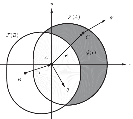
Let be the expected number of nodes in whose potential is greater than that of , so that
| (3) | |||||
where is the infinitesimal area element corresponding to , and the indicator function is equal to if the condition holds and to if it does not.
Also, let denote the probability of the event that does not contain an eligible node, i.e., that a new buffering stage will commence at the moment node receives the packet. This event will occur if there are no nodes in whose potential is greater than the potential of . The number of such nodes has a Poisson distribution with mean , therefore,
| (4) |
Finally, let be the joint density of the location and the travel direction of the eligible node to which the packet is immediately transmitted from (see Fig. 1), so that is equal to zero if no such node can exist for the given choice of and . In order to obtain a useful expression for for all , , first observe that if , i.e., node is at least as suitable as node for keeping the packet. We also have if , i.e., is in the intersection of the FRs and and so no eligible node may be found there by the Second-Order Approximation.
When both and , the joint density of the location and direction of node is , and will receive the packet if there is no other node in that is better than . The expected number of such nodes is (cf. with the derivation of (3))
where, as before, is the infinitesimal area element corresponding to , and as their number is Poisson distributed, we have
Combining all cases, we have
| (5) |
Observe that, for all , , we must have
| (6) |
This is due to the fact that, upon the reception of a packet, either a sojourn will start, or another transmission will take place, with probability .
V Buffering Stage Analysis
As the second step of the analysis, in this section we compute explicit expressions for a number of quantities related to what follows a buffering stage. Specifically, suppose that at time a buffering stage starts with the packet in the buffer of a node , and traveling in direction . The buffering ends at time , for some .
We partition the event corresponding to the end of the buffering stage into four families of disjoint events, each one describing a different manner in which the buffering will end. We then use our second approximation, introduced in Section V-D, to compute the probability of each of these events.
V-A Four families of events
Given the value of , first we define the collection of events
where is the event that the buffering ends because, at time , node changes its travel direction from to , while no eligible node is found. Second, we let
where is the event that the buffering ends because, at time , node changes its travel direction from to some and an eligible node is immediately found in location and traveling in direction .
The third collection of events we will consider is
where is the event that the buffering ends because, at time , while is still traveling in direction , a node located at changes direction from some previous to , thus becoming eligible.
To define the fourth family, we first need to introduce another mild assumption on the FR and the potential , complementing the assumptions of Section III-C regarding the RR. For any , let denote the subset of the FR of a node traveling in direction , where ; cf. Fig. 2. Therefore, nodes that enter from the outside immediately become eligible.
Assumption 3. We assume that, for any , the region is convex. Let the threshold curve, , parametrized by , be the curve separating and . We assume that the curvature of is uniformly bounded, in that is differentiable with respect to , for almost every , and there exists a finite constant , independent of , such that the magnitude of the derivative with respect to is bounded by :
Note that Assumption 3 implies that the length of the curve is bounded, a property which is obviously satisfied for any reasonable choice of the potential , provided the parametrization is suitably chosen. [For concreteness, we also mention that the derivative with respect to above is taken on the - and -coordinates of .] Let denote the unit vector perpendicular to the curve at the location specified by , and pointing in the direction of lower potential. Observe that changing to traces an infinitesimal line segment of length that is perpendicular to ; see Fig. 2. Clearly, a node that “hits” the curve from outside immediately becomes eligible.

We can now define the last collection of events of interest here:
where denotes the event that the buffering ends because, at time , an eligible node appears at the position of the boundary of corresponding to , traveling with direction . Finally, we write
and we note that , i.e., these four cases cover every possible scenario, with probability 1.
V-B Transition rates
Let , and arbitrary, let denote the infinitesimal area element in location as before, and let . With a slight abuse of notation we define the transition rates , , , and , as:
| (7) | |||||
| (8) | |||||
| (9) | |||||
| (10) |
Intuitively, these rates describe the infinitesimal probability that a buffering stage will end exactly in each one of the four possible scenarios discussed above, after an infinitesimal duration of time . Formally, we could define , via the limit
as , and similarly for the other three transition rates. We now proceed to derive expressions for each of them, in terms of the network model and the RR parameters specified earlier; cf. Table II. Again, with a slight abuse of terminology and notation, in the subsequent discussion we omit the adjective “infinitesimal” most of the time, e.g., referring to the quantities in the right-hand sides of (7)–(10) simply as “probabilities.”
Regarding , the probability in the right-hand side of (7) is equal to the product of five different quantities: the probability that node will change its direction during that interval; the probability that will pick direction ; the probability that there are no eligible nodes in with potential at most but greater than , which is (recall the derivation of (4)),
the probability, , say, that no event in will occur before ; and the probability, , say, that that no event in will occur before .
Now observe that is bounded below by the probability that no node in a region of area will change travel direction in a time interval of duration . As for , we claim that it is bounded below by , where is the bound to the length of the curves specified by Assumption 3. Indeed, the expected number of nodes with a given travel direction and density that cross , whose length is less than , in a time interval , with a relative speed less than , is less than . Integrating over all , it follows that the expected number of all such nodes is less than . As the distribution of their total number is Poisson, the probability that no node will cross some curve in a time interval is greater than , and so . We note that similar arguments can be used in the calculation of the other three transition rates to show that the probability that an event of a different type occurs does not affect the rate; as these arguments are straightforward, they will be omitted.
Combining the above estimates and ignoring terms of order , it follows that
| (11) |
Regarding , note that, if , then the probability in the right-hand side of (8) is zero because the condition implies that there was an eligible node before changed direction. However, if , then this probability can again be expressed as the product of four different terms: the probability that node will change its travel direction during the interval ; the probability
that its new direction will lead to a lower potential than (otherwise, the packet would have stayed with ); the probability that there is a node at the specified location with the specified travel direction ; and the probability that there is no node in that is better than that node, which is (cf. with the derivation of (4))
Therefore,
| (12) |
Regarding , the probability in the right-hand side of (9) is zero when . Otherwise, it is equal to the probability that there is a node within the specified area,
multiplied with the probability that that node will turn to direction . Therefore,
| (13) |

Regarding rate , observe that nodes that move in direction appear to node to be moving with relative speed ; cf. Fig. 3. Also observe that, in order for the probability on the right-hand side of (10) to be nonzero, the inner product must be negative (as shown in the figure) so that nodes with travel direction are hitting the boundary from the outside of . Then, this probability is equal to the density of nodes traveling in direction , multiplied with the area of the parallelogram (which appears shaded in the figure) with sides of length and , at an angle . Therefore,
and noting that the inner product,
we obtain:
| (14) |
Having computed expressions for , , , and , we finally define one last family of transition rates that will be used in subsequent derivations. First, given the value of as before, we define the family of events
where is the event that the buffering ends because, at time , an eligible node appears at position on the curve , traveling in direction . Also we define the transition rates
Observe that is simply a different representation of , and it can be easily recovered from knowing and . Indeed, fixing and , the rate only specifies the transition rates of eligible node arrivals but not their locations; these are provided by the function ; on the other hand, the rate already contains this information. In particular, we have
| (15) |
for any , with .
In our numerical calculations later or, we calculate the rate , for a specific pair and for all , as follows. First, we discretize , defining values , to cover , each associated with an interval of length , , the intervals partitioning . Then, we discretize , defining values , , each associated with an area , the areas partitioning . We map each to the location nearest to , and we denote the resulting map by . And setting
we have a discretized version of (15).
V-C Aggregate rates
We also define the aggregate rates , , , , and as follows:
| (16) | |||||
| (17) | |||||
| (18) |
The interpretation of the first four rates above is that, each one of them, multiplied by , is the infinitesimal (conditional) probability that an event from the corresponding family will occur after a time , given that the packet is traveling in direction . And the last one rate, , multiplied by , gives the probability that the buffering of stage will end after a time , given that .
Observe that we must have
as the union of the events belonging to the families and is the event that node changes direction, which happens with rate . Therefore,
| (19) |
V-D Time-Invariance Approximation and consequences
The transition rates of the events in the four families defined in Section V-A are not independent of the duration of the buffering stage. Intuitively, as time progresses, memory accumulates, and the probability of each of them occurring changes. As this fact significantly complicates the analysis required for computing the probability that a specific one of these events occurs, we adopt the following simplifying assumption:
Time-Invariance Approximation: For each incremental event , and any time , as we have:
Intuitively, under this approximation, the probability that the buffering will end in a specific manner does not change as the stage progresses, but it is equal to the probability that this will happen right at the moment when the buffering starts (and the mobility process has been restarted, due to the Second-Order Approximation). In particular, integrating the above expression over all implies that is memoryless, in that
therefore, under the Time-Invariance Approximation, each is exponentially distributed [27] with rate .
Furthermore, the Time-Invariance Approximation makes it possible to obtain “time-averaged” versions of the expressions for the rates in (7)–(10). For example, adopting the same slight abuse of notation as before, for any event we have
where the third equality follows from the Time-Invariance Approximation, and the last equality from the definition of and the fact that, conditional of , is exponential with rate . Integrating over , we then obtain
Working in the same manner for the other families, we can arrive at similar results. Summarizing,
| (20) | |||||
| (21) | |||||
| (22) | |||||
| (23) | |||||
| (24) |
VI Performance Metrics
In this section we will derive expressions for the long-term average packet speed and cost induced by our RR on this network model. These will be expressed in terms of the invariant distribution of an appropriately defined Markov chain. The following is the last technical assumption we need to impose on the potential function:
Assumption 4: The value of is equal to a constant for all .
Coupled with the monotonicity of , this assumption simply states that the direction is uniformly the worst, irrespective of the location of a candidate neighbor. Note, however, that the behavior of as a function of can strongly depend on , so that ‘good’ locations can be favored, in terms of the potential assigned to them, as long as nodes at those locations are not traveling in direction . Therefore, this assumption is clearly not significantly restrictive. In technical terms, it will be used to establish the irreducibility of the chain defined below. As should become evident from the analysis, this assumption could be relaxed, but at the cost of significantly complicating some of the arguments involved, so we will not pursue this direction further.
VI-A The Markov chain
We define the state associated with each stage , by if is a wireless transmission stage, and by if is a buffering stage. The associated state space in which each takes values is , where the transmission state space
and the buffering state space
By Assumptions 1 and 4, a node traveling in direction will never receive a packet from a node , irrespective of its location and node ’s traveling direction, therefore the pairs with are not included in .
Observe that, due to the Second-Order Approximation, the process forms a Markov chain: If , i.e., is a buffering stage, then at the start of that stage the complete mobility model was restarted, except that the carrier kept its travel direction and its FR did not contain nodes with a potential higher than that of , i.e., . Likewise, if with , i.e., in stage the packet is transmitted from a node to a node located at , then, at the moment received the packet, the whole mobility model was again restarted, except that kept its travel direction and all nodes with potential higher than were expunged from . In both cases, the complete information remaining about the network is captured in the current state.
The distribution of the chain may be described as follows. We assume that is an arbitrary initial state, and for each , given , the chain moves to a state according to the following family of conditional distributions, as derived in the previous section: If , the conditional density of is
if and , the conditional density of is
if both and are nonzero, then the conditional density of is
where the function is given in (5); and finally, if and , then the conditional density of is
In the sequel we refer to , , , and as the kernel functions, since they can be used to fully specify the transition kernel of the chain .
VI-B Ergodicity
In this section we establish that, under the Second-Order Approximation, the Time-Invariance Approximation, and Assumptions 1–4, the Markov chain is ergodic, with a unique invariant distribution , to which it converges at a geometric rate.
Let denote the Lebesgue measure on , denote the Lebesgue measure on , and be the point mass at point . We write for the measure , defined on the state space , equipped with the usual Borel -field. Our first result describes the long-term behavior of the chain , and its consequences are stated in detail after that; see [28] for some relevant background on Markov chains. Theorem 1 is proved in the Appendix.
Theorem 1
Under the Second-Order Approximation, the Time-Invariance Approximation, and Assumptions 1–4, the Markov chain is -irreducible, aperiodic, and uniformly ergodic on the state space , with a unique invariant measure to which it converges uniformly geometrically fast. In particular:
- 1.
There are constants and such that, for any initial state ,
for all and any (measurable) set .
- 2.
For any (measurable) function with , as we have, with probability one,
for any initial state , where .
An important ingredient in the proof of Theorem 1 is the following domination condition, which will be verified in the Appendix. Intuitively, Lemma 1 says that, irrespective of the current state, with probability at least the chain will be in a uniformly distributed buffering state after two time steps.
Lemma 1
(Doeblin condition) Let denote the measure on . There is an such that for any (measurable) and any , we have:
Another ingredient of the proof of the -irreducibility part of Theorem 1 is provided by the following one-step reachability bound. Lemma 2 is proved in the Appendix.
Lemma 2
Let denote the measure on . For any (measurable) with there are such that,
| (25) |
The main implications of Theorem 1 for our results are stated in the following corollary, which is proved in the Appendix. In order to state it we need some additional definitions. Given an arbitrary state in , let be exponentially distributed with rate if , and otherwise. Similarly, for each , given and , let have the same distribution as given . Then defines a new Markov chain, on the state space:
Now suppose has distribution and let be defined as before, conditional on . Write for the induced joint distribution of on .
Corollary 1
For any initial state , , the following ergodic theorems hold with probability one:
where so that, in particular, .
As the final step of our analysis, we provide expressions for the performance metrics defined in Section III-E. The following results, stated without proof, are immediate consequences of Corollary 1.
Corollary 2
Some details regarding the numerical computation of expectations under and are given in Section -B of the Appendix.
VII Numerical Results
In this section, we compare the approximate results for the performance metrics and obtained in previous sections, with corresponding simulation results for specific choices of the FR and the potential function .
VII-A Setting
We consider the potential function
so the packet constantly tries to find nodes with a good travel direction, regardless of their relative location, provided, of course, they are within the FR. The FR we consider is specified by the boundary function
for some , , so that is an ellipse whose major axis, of length , is along the -axis, its left focus is at the origin, and its eccentricity is . The boundary function is drawn in Fig. 4 for a few different choices of the parameters and . Note that larger values of make the routing protocol more aggressive in finding nodes to send the packet to, whereas larger values of make the routing protocol more selective regarding the relative locations of neighboring nodes. In the important special case , is a circle of radius , so that the routing protocol gives the packet to any node with a direction better than that of the current holder, as long as the two nodes are within distance of each other. This choice of boundary function may be the only possible if the nodes only know their travel directions but not their relative locations, and they can exchange packets whenever they are within a communication radius of each other.


Finally, we assume that the transmission cost is quadratic, , and for the density of the travel direction we take
where . Therefore, is positive and constant on four intervals centered in the directions of the positive and negative - and -axes, whereas outside of these ranges is zero. For , the density is the uniform density , for all directions . At the other extreme, small values of model situations in which all nodes move along the direction of one of two perpendicular axes; this would happen, for example, with a vehicular network of nodes moving in a rectangular road grid. In Fig. 4 we also plot the density for three different values of the parameter . In Table III we collected all the quantities used in the calculations of this section, along with their default values; these values are used in all computations, unless explicitly stated otherwise.
| Quantity | Symbol | Default value |
|---|---|---|
| Node density | ||
| Direction density | (uniform) | |
| Node speed | ||
| Node turning rate | ||
| Transmission cost | N/A | |
| Boundary function | , | , |
| Potential | , , | N/A |
VII-B Results
Fig. 5 shows the effects of the shape of the FR (as the eccentricity and the half-axis length vary) on the packet speed and the packet cost . Here, and in all subsequent figures, the results obtained from our earlier analysis are shown as solid black lines, and the corresponding simulation results are shown as dotted red lines.


Observe that, as the half-axis length increases, the packet speed increases but so does the packet cost; this exemplifies the fundamental trade-off between these two metrics. The increase in the speed as gets larger is because it becomes more likely for a node with a good travel direction to be available when the carrier changes direction to a bad one, and also (when ) because that node is farther ahead on the average; for the same reason, and also because the transmission cost function is quadratic, also increases as increases. In fact, as the figure suggests, we expect that when , the speed diverges to infinity as increases, since the expected progress per wireless transmission increases with . On the other hand, the cost diverges to infinity, as increases, even when .
Regarding the effects of the eccentricity , observe that, starting from and increasing it, initially leads to higher speed and lower cost. This is natural, as the value corresponds to a circular FR, therefore neighboring nodes whose relative position is towards the positive -axis are not given preference; this inefficiency is rectified as initially increases. However, increasing past actually leads to an increase in the cost. Indeed, if the FR is too elliptical, it often happens that the packet is transmitted to nodes that are too far away from the current carrier, albeit with an excellent relative position, although there were other nodes that were much closer to the carrier with a relative position almost as good; as the cost is quadratic, this inevitably increases the packet cost. Large values of the eccentricity also hurt the speed because, when increases, the area of the FR is reduced (the exact formula is ), and the packet spends more time traveling towards relatively bad directions on the buffers of nodes.
In Fig. 6 we plot the values of and versus the two node parameters, namely, the node density and the node turning rate .


Regarding the effects of , we first observe that, when is very small, as long as the node density is not very small, the packet speed is almost equal to the node speed. Indeed, the packet stays with a node with a near-perfect direction for a significant amount of time, and in the infrequent cases when that node changes its direction, another one will be found within a relatively short time. Consequently, the packet cost is also very small. On the other hand, when is not very small, then, the larger is, i.e., the more frequently a node changes direction, the more frequent are the transmissions to nodes with better directions, and hence both the packet cost and the speed get larger; this effect on the speed crucially depends on the fact that transmissions are, on average, towards the direction of the positive -axis, since, in this figure, we use the default value .
Regarding the effects of , when is fixed and non-negligible, a low density leads to low packet speed, as the packet spends extended periods of time traveling towards bad directions; on the other hand, a large node density means that the packet travels fast, due to frequent transmissions. However, this effect diminishes as, after a while, a node with near-perfect travel direction is guaranteed to exist within the FR whenever the current carrier changes its travel direction; therefore, increasing the density further has no effect. On the other hand, is near-constant as changes. To understand this, compare the high-density regime with the low-density regime: In the first case, the travel of the packet consists of wireless transmissions and physical transports in the right direction. In the second case, it again consists of wireless transmissions and transports in the right direction, but also involves extended periods of transports in random directions (which, on the average, produce no progress). The two cases differ significantly in their performance in terms of progress per unit time (i.e., the speed) but not in terms of cost per unit distance (in the positive -axis direction), as transports in random directions have an approximately zero net effect.
Finally, in Fig. 7 we plot and versus the angular width and the size of the half-length, when , i.e., the FR is a circular disk.


Once again we observe that, as in Fig. 5, increasing increases both the speed and the cost. Indeed, the more nodes there are in the FR, the higher is the probability that, once the packet changes its travel direction, another node with a good travel direction will be available. However, in contrast to Fig. 5, as increases the effects on the speed tend to diminish; indeed, after some value of , the probability that an eligible node with a good direction exists is invariably close to unity, and because now the eccentricity , wireless transmissions have a zero net effect on the speed of the packet, which does not change with .
As for , its effects are much less pronounced: Both and change little with . This can be justified by observing that changing does not make the directions with which the nodes travel overall better, only differently distributed; still, the effects of on the performance metrics are remarkably small.
Finally, we note that the discrepancy between the simulation results and our analytical results is generally small and almost always modest. One exception is the setting of Fig. 7 in the cases of both small values of and large values of , where the discrepancy is significant. However, this discrepancy is not due to the inaccuracy of our two simplifying approximations but, rather, due to accumulating numerical errors. Specifically, in this regime, the errors due to the discretizations used are large, because there is a non-negligible probability that there will be two or more nodes in the FR with the exact same (discretized) travel direction and, hence, potential once a packet arrives at a new node or its current holder changes direction; note that our analysis assumes that the probability of this event is zero. Excepting this case, the discrepancy between simulations and analysis remains modest, although it does increase with (cf. Fig. 6). Indeed, as increases, the Second-Order Approximation is invoked more frequently, and the estimated rates with which the FR encounters eligible nodes deviate more from the actual ones.
VIII Conclusions
In this work, we first introduced a mobile wireless DTN model in which nodes move on the infinite plane, according to a random waypoint mobility model, and a packet must travel to a destination located at an infinite distance away according to a routing rule that is using both wireless transmissions and physical transports on the buffers of nodes. The routing rule is defined in terms of a forwarding region and a potential function; specifying these leads to different versions of the routing rule. This model is quite general, notably including cases where the transmission cost depends on the direction of the transmission, arbitrary distributions for the direction of node travel, and a large variety of routing rules.
In this setting, we defined two performance metrics: the speed with which the packet travels to its destination, and the rate with which the transmission cost is accumulated. We computed these performance metrics by adopting two simplifying approximations. These approximations ensure that a simpler discrete-time Markov chain embedded in the system description can be analyzed using general tools from Markov chain theory. The assumptions are intuitive, and furthermore are shown to introduce modest errors, on the order of no more than 10%, in the examples considered in our numerical evaluations.
The present results help quantify the important trade-off that exists in mobile wireless DTNs between the speed with which packets travel to their destinations and the rate with which the transmission cost is accumulated. Also, the methodology we have developed may be extended in a variety of directions, e.g., to include the case where the velocity magnitude is not constant and the duration of time a node spends with a given travel direction depends on its velocity vector. Alternatively, the present development may also be used as a starting point for more accurate analytical approaches, e.g., maintaining more memory in each stage of the Markov chain. Related work on much simpler settings [22] suggests that dispensing with approximations altogether might be a formidable task.
An interesting potential application of our work is towards studying the performance of non-delay-tolerant geographic routing protocols. Consider, for example, a simple RR with a circular FR of radius , and such that when , with probability going to there will be an eligible node whenever a packet arrives at a new node; therefore, as increases physical transports become less and less frequent. Taking the limit as of the cost readily gives the performance of a non-delay-tolerant geographic routing protocol.
Regarding future work, the present setting naturally leads to the problem of finding the best routing rules, e.g., those that achieve Pareto optimal combinations of delays and costs. Tackling this problem with tools from genetic algorithms or multi-armed bandit theory jointly with tools from stochastic geometry might be a fruitful strategy. Also, the assumption that all nodes travel with the same speed is not crucial and could be relaxed; for example, we could use a more general model under which each node travels, independently of all others, with a speed that is constant between the times the node changes direction, but the speed changes when the direction changes, and speeds associated with consecutive trajectory segments are independent random variables following some given distribution. Likewise, we could assume that the distribution of the duration of time a node spends with a given travel direction does depend on that direction. On the other hand, two other aspects of our model, namely, the independence of node trajectories and the changes of each node’s directions according to a Poisson process, cannot be easily relaxed, as that would introduce new sources of memory, making it more difficult to develop an accurate and tractable Markov chain model for the packet trajectory.
In the first section of the Appendix we give the proofs of the theoretical results in Section VI. In the other sections we provide details on the numerical evaluation of the performance metrics and intermediate results.
-A Proofs
Below we establish Theorem 1, Lemmas 1 and 2, and Corollary 1. In several parts of the proofs where we need to invoke technical but quite standard arguments, some of the details are omitted.
Proof of Lemma 1: It is obvious that it suffices to establish the result of the lemma for events of the form , for . And by the uniqueness of Carathéodory extension, since the collection of all finite unions of intervals forms an algebra that generates the Borel -algebra of , it further suffices for to only consider closed intervals, ; see, e.g., [29, 30] for details. So in the rest of the proof we restrict attention to events of the form .
Also note that, from the expressions derived in Section V-B, it is simple to obtain the following bounds on the transition rates , , , , and on :
| (28) | |||||
| (29) |
We note that is a lower bound on defined in Section III-A.
Now, if is of the form for some , then for any ,
so that, using the lower bound in (28) and the upper bound in (29), we have that, for some fixed constant :
| (30) |
Then, using the Markov property and applying (30) twice,
| (31) | |||||
Similarly, if is of the form for some and , then by the Markov property,
and recalling the expression for in (3) we clearly have , so that,
| (32) |
Proof of Lemma 2: Since has positive Lebesgue measure, we can find a rectangle of the form with a nonempty interior, such that . The idea of the main argument here is to show that there is a range of angles such that, when the current packet holder travels with a direction in , there is a strictly nonzero probability that there are ineligible nodes in that can become eligible by changing their travel direction to a better one within the range .
Since is continuous, the image of is a closed interval . And since has a nonempty interior, we must have by Assumption 1. Also, by Assumptions 1 and 4, and noting that in order to have , we must have .
Next, pick such that , and let and be such that and ; such angles are guaranteed to exist by the intermediate value theorem. Also, observe that is continuous on the compact set , so it is uniformly continuous there, which implies that there is a with for all and all .
Now take and arbitrary. We will bound , given by (13), from below. First note that and , therefore . Also, we have for all . Therefore,
| (33) |
where the second inequality follows by the fact that is assumed bounded below by (cf. Section III-A). Also recall that is bounded above as in (29).
We are now ready to prove the inequality (25). For any , where the interval is chosen above,
| (34) |
The last integral is strictly positive because is nonzero, is bounded away from zero by (33), and is bounded above by (29). ∎
Proof of Theorem 1: First we will establish the -irreducibility and aperiodicity [28] of the chain . In fact, we will show that, for any and any state , the measure is absolutely continuous with respect to the measure . To that end, choose and fix an arbitrary state and an arbitrary measurable subset of with , so that either or (or both).
In the first case, Lemma 1 implies that for any , which, together with the Markov property, implies that for all . In the second case, combining Lemma 1 with Lemma 2 applied to and with the Markov property, we obtain that there are such that
where the positivity of the last integral follows again from Lemma 2. Finally, using the Markov property once again, we have that for all , as required.
Now, -irreducibility and aperiodicity, together with the Doeblin bound of Lemma 1, imply [28, 31], that the chain is uniformly ergodic. Specifically, Lemma 1 implies that the state space is small, and that the drift condition (V4) of [28] holds with Lyapunov function . Then [28, Theorem 15.0.1] implies that the chain has a unique invariant (probability) measure to which the distribution of converges uniformly, as stated in part of the theorem. In particular, the chain is Harris recurrent, and [28, Theorem 17.0.1] implies that the strong law of large numbers holds for functions , as stated in part of the theorem. ∎
Proof of Corollary 1: Since and are bounded, and hence -integrable, functions of , the first two results immediately follow from Theorem 1. For the next two, let denote the measure on . Arguing as in the proof of Theorem 1, it is easy to show that the new chain is -irreducible and aperiodic, and also uniformly ergodic. Once again, [28, Theorem 17.0.1] implies that the strong law of large numbers holds for , and recalling that , the last two statements of the corollary will follow as soon as we establish that is -integrable. Indeed, since, given , is exponential with rate , we have
completing the proof. ∎
-B The invariant distribution and expectations under ,
Let , , be the density of under , so that we think of is the long-term infinitesimal proportion of time that . Similarly, let , , denote the joint density of under , so that we think of as the long-term infinitesimal proportion of time that , where is the infinitesimal area element centered at r. In order to compute the functions and , we derive balance equations, as follows.
First, note that the proportion of state transitions out of is . This should be equal to the proportion of transitions into , for which we observe that the proportion of transitions out of is equal to , and of these a proportion transitions to states inside . Likewise, the proportion of transitions out , where is the infinitesimal area element centered at of size , is . Of these, a proportion enters . Therefore, integrating over all relevant state transitions we have
| (35) |
Second, observe that the proportion of transitions out of is . This should be equal to the proportion of transitions into that set. To compute that, we observe that the state is in for a proportion of time equal to and, at these instances, a proportion of transitions equal to
is into . Likewise, the proportion of transitions out of is . Of these, a proportion enters . Again, integrating over all relevant state transitions we obtain,
| (36) |
In order to compute and , we discretize their arguments, which converts the balance equations (35) and (36) into a large linear system; we also use the fact that the sum of their integrals should be equal to unity; see Section -G for details.
Then, having and , we can readily derive the following expectations with respect to the invariant distribution of the chain:
where the inner variable of integration in the first integral is .
-C Numerical computation of integrals
In a number of instances in this work we need to compute the values of a multivariate function that is given as a multiple integral. A good example is (3), which is of the following form:
| (37) |
We show how we calculate this integral; all other similar integrals in this work are calculated using the same method, mutatis mutandis.
First, we discretize the variable , considering only the values,
| (38) |
where is a positive integer. Second, we discretize , by placing points uniformly inside . This is achieved as follows: we create points,
| (39) |
where is a positive integer, and the parameter is such that the region (which we have assumed bounded) lies entirely within the square ; then, we keep those points that are within the region , denoting them as,
| (40) |
in polar and Cartesian coordinates respectively.
Then, we restrict ourselves to calculating for all , , and equation (37) becomes,
| (41) |
This integral is calculated approximately as follows: We associate with each point , , , the rectangle,
| (42) |
of volume,
| (43) |
so that these rectangles approximately partition the set over which the integral (41) is taken. And finally we set:
Clearly, the larger and are, the closer this approximation to the true values of .
-D Speeding up the computation of
A time-consuming part of the computations required for our numerical results is the repeated calculation of using (3). Indeed, is a function of two variables, and finding each of its values requires the evaluation of a multiple integral. However, assuming that the potential function is only a function of makes this computation simpler. Indeed, in this case we have,
where,
| (44) | |||||
| (45) |
Both of these integrals can be computed beforehand for all necessary values of and , either numerically or analytically, and be readily available when the calculation of starts.
Furthermore, when then we have an even simpler expression for :
-E Speeding up the computation of
Another time-consuming part of our computations is the calculation of , using (5). This is because is a function of four variables, and each of its values requires the evaluation of a multiple integral. The calculation can be significantly simplified if we take into account any special structure of the FR and the potential function. For example, if is only a function of , then (5) simplifies to,
-F Speeding up the computation of
One final computational bottleneck is the calculation of using (12), because it is a function of three variables and calculating any of its values again involves the evaluation of a multiple integral. Considering, as before, the case where the potential is a function of only, the first integral in (12) becomes,
where,
Furthermore, the multiple integral in (12) becomes,
where is the area of , and,
In order to speed up the relevant calculations, , , and can be computed once in the beginning, and made available when the calculation of starts.
-G Numerical solution of (35) and (36)
Finally, here we describe the numerical solution of the system of balance equations (35) and (36) derived in Section -B of the Appendix above. As discussed there, we restrict ourselves to computing and only for the discrete sets of values of and given in (38) and (39), respectively, so that (35) and (36) become,
for and . Then we perform a piecewise constant approximation of the integrands in the rectangular sets (42), with the constant values being the values of the integrands at their centers. And taking the integral over the union of these rectangles, we get,
where and . Multiplying the first equation by , the second equation by , and defining, with a slight abuse of notation,
and likewise for all other functions appearing in the balance equations, we obtain the system,
for and . This is a linear system of equations, which may be interpreted as expressing the balance equations of a discrete Markov chain with states (because (6) and (18) ensure that the probabilities of transitions out of each state indeed add up to unity in all cases). To solve this system, we write it in the form , where is a vector of length consisting of followed by each of the columns of . Since the resulting matrix is stochastic, by construction, we find an eigenvector corresponding to its top eigenvalue, which, after normalization, provides the required solution.
References
- [1] R. Cavallari, R. Verdone, and S. Toumpis, “Cost/speed analysis of mobile wireless DTNs under random waypoint mobility,” in Proc. Wiopt, Tempe, AZ, May 2016.
- [2] R. Cavallari, S. Toumpis, and R. Verdone, “Analysis of hybrid geographic/ delay-tolerant routing protocols for wireless mobile networks,” in Proc. IEEE INFOCOM, Honolulu, HI, Apr. 2018.
- [3] I. Kontoyiannis, S. Toumpis, R. Cavallari, and R. Verdone, “On calculating packet speed ad cost in a mobile wireless network model,” 2018, submitted to IEEE ISIT 2018.
- [4] A. Vasilakos, Y. Zhang, and T. V. Spyropoulos, Eds., Delay Tolerant Networks: Protocols and Applications. CRC Press, 2011.
- [5] P. Gupta and P. R. Kumar, “The capacity of wireless networks,” IEEE Trans. Inf. Theory, vol. 46, no. 2, pp. 388–404, Mar. 2000.
- [6] M. Grossglauser and D. N. C. Tse, “Mobility increases the capacity of ad-hoc wireless networks,” in Proc. IEEE INFOCOM, vol. 3, Anchorage, AL, Apr. 2001, pp. 1360–1369.
- [7] S. Diggavi, M. Grossglauser, and D. N. C. Tse, “Even one-dimensional mobility increases the capacity of wireless networks,” IEEE Transactions on Information Theory, vol. 51, no. 11, pp. 3947–3954, 2005.
- [8] S. Toumpis and A. J. Goldsmith, “Large wireless networks under fading, mobility, and delay constraints,” in Proc. IEEE INFOCOM, Hong Kong, China, Mar. 2004.
- [9] G. Sharma, R. Mazumdar, and N. Shroff, “Delay and capacity trade-offs in mobile ad hoc networks: a global perspective,” IEEE/ACM Trans. Netw., vol. 15, no. 5, pp. 981–992, Oct. 2007.
- [10] P. Jacquet, S. Malik, B. Mans, and A. Silva, “On the throughput-delay tradeoff in georouting networks,” IEEE Trans. Inf. Theory, vol. 62, no. 6, pp. 3230–3242, June 2016.
- [11] P. Jacquet, B. Mans, and G. Rodolakis, “Information propagation speed in mobile and delay tolerant networks,” IEEE Trans. Inf. Theory, vol. 56, pp. 5001–5015, Oct. 2010.
- [12] Y. Li and W. Wang, “Message dissemination in intermittently connected D2D communication networks,” IEEE Trans. Wireless Commun., vol. 13, pp. 3978–3990, July 2014.
- [13] E. Baccelli, P. Jacquet, B. Mans, and G. Rodolakis, “Highway vehicular delay tolerant networks: Information propagation speed properties,” IEEE Trans. Inf. Theory, vol. 58, no. 3, pp. 1743–1756, March 2012.
- [14] M. Zarei, A. M. Rahmani, and H. Samini, “Connectivity analysis for dynamic movement of vehicular ad hoc networks,” Wireless Networks, 2016.
- [15] E. Baccelli, P. Jacquet, B. Mans, and G. Rodolakis, “Multi-lane vehicle-to-vehicle networks with time-varying radio ranges: Information propagation speed properties,” in Proc. IEEE ISIT, Istanbul, Turkey, July 2013.
- [16] J. LeBrun, C.-N. Chuah, D. Ghosal, and M. Zhang, “Knowledge-based opportunistic forwarding in vehicular wireless ad hoc networks,” in Proc. IEEE VTC Spring, vol. 4, Stockholm, Sweden, May-June 2005, pp. 2289–2293.
- [17] K. Peters, A. Jabbar, E. K. Çetinkaya, and J. P. G. Sterbenz, “A geographical routing protocol for highly-dynamic aeronautical networks,” in Proc. IEEE WCNC, Cancun, Mexico, Mar. 2011, pp. 492–497.
- [18] A. G. Tasiopoulos, C. Tsiaras, and S. Toumpis, “Optimal and achievabnle cost/delay tradeoffs in delay-tolerant networks,” Computer Networks, vol. 70, pp. 59–74, Sep. 2014.
- [19] P. Madadi, F. Bacelli, and G. de Veciana, “On temporal variations in mobile users SNR with applications to perceived QoS,” in Proc. Wiopt, Tempe, AZ, May 2016.
- [20] B. Liu, P. Brass, O. Dousse, P. Nain, and D. Towsley, “Mobility improves coverage of sensor networks,” in Proc. ACM MobiHOC, Urbana-Champaign, IL, May 2005, pp. 157–162.
- [21] Y. Peres, A. Sinclair, P. Sousi, and A. Stauffer, “Mobile geometric graphs: Detection, coverage, and percolation,” Probab. Theory Relat. Fields, vol. 156, no. 1, pp. 273–305, 2013.
- [22] D. Cheliotis, I. Kontoyiannis, M. Loulakis, and S. Toumpis, “Exact speed and transmission cost in a simple one-dimensional wireless delay-tolerant network,” in Proc. IEEE ISIT, Aachen, Germany, June 2017.
- [23] A. Sidera and S. Toumpis, “Delay tolerant firework routing: a geographical routing protocol for wireless delay tolerant networks,” Eurasip Journal on Wireless Communications and Networking, Feb. 2013.
- [24] ——, “On the delay/cost tradeoff in wireless mobile delay-tolerant networks,” in Proc. Wiopt, Tempe, AZ, May 2014.
- [25] F. Baccelli and B. Blaszczyszyn, Stochastic Geometry and Wireless Networks, Vols I-II. Foundations and Trends in Networking, 2009.
- [26] A. Ephremides, “Energy concerns in wireless networks,” IEEE Wireless Commun. Mag., vol. 9, no. 4, pp. 48–59, Aug. 2002.
- [27] S. Ross, Stochastic Processes. New York, NY: John Wiley and Sons, Jan. 1995.
- [28] S. Meyn and R. Tweedie, Markov Chains and Stochastic Stability, 2nd ed. London: Cambridge University Press, 2009, published in the Cambridge Mathematical Library. 1993 edition online: http://probability.ca/MT/.
- [29] H. Royden, Real Analysis. New York: Macmillan, 1988.
- [30] D. Williams, Probability with martingales. Cambridge university press, 1991.
- [31] I. Kontoyiannis and S. Meyn, “Spectral theory and limit theorems for geometrically ergodic Markov processes,” Ann. Appl. Probab., vol. 13, pp. 304–362, February 2003.