Neutral and charged (pseduo)scalar mesons and diquarks under magnetic fields

We investigate the (pseudo)scalar mesons and the diquark in the scalar channel by using a low energy approximation of QCD effective model SU(2) NJL model under an external magnetic field, the Lagrangian is given by[41, 42]

Where $\psi$ represents the quark field of two light flavors $u$ and $d$, the current mass matrix $\hat{m}=\text{diag}(m_{u},m_{d})$, we can assume that $m_{u}=m_{d}=m_{0}$. $\tau^{a}=(I,\vec{\tau})$ with $\vec{\tau}=(\tau^{1},\tau^{2},\tau^{3})$ corresponding to the isospin Pauli matrix. $G_{S}$ is the coupling constants corresponding to the (pseudo)scalar channel. The covariant derivative, $D_{\mu}=\partial_{\mu}-iQeA_{\mu}^{ext}$, couples quarks to an external magnetic field $\bm{B}=(0,0,B)$ along the positive $z$ direction via a background field, for example, $A_{\mu}^{ext}=(0,0,Bx,0)$ and the field strength tensor is defined by $F_{\mu\nu}=\partial_{[\mu}A_{\nu]}^{ext}$, $Q=(-1/3,2/3)$ is a diagonal matrix in the flavor space which respects to the electric charge of the quark field ($u,d$).

Semi-bosonizing the above Lagrangian and the Eq.(1) can be rewritten as

where the Euler-Lagrange equation of motion for the auxiliary fields leads to the constraints as follows:

For each flavor, by introducing the chirality projector $P_{L}=\frac{1+\gamma^{5}}{2}$ and $P_{R}=\frac{1-\gamma^{5}}{2}$, we have

and for two-flavor spinor $\bar{\psi}=(\bar{u}\ \ \bar{d})$, the auxiliary neutral scalar and pseudo scalar $\sigma$ and $\pi^{0}$ can be written as follows:

It is obviously to find that the neutral scalar $\sigma$ is symmetric in the flavor space, while the neutral $\pi^{0}$ is anti-symmetric in the flavor space and keeps as a pseudo Goldstone mode. The charged $\pi^{\pm}$ can be represented as:

with $\tau^{\pm}=\frac{1}{\sqrt{2}}(\tau_{1}\pm i\tau_{2})$.

The quark-antiquark condensation which gives quark the dynamical mass and the constituent quark mass is obtained as

We should minimize the effective potential in order to obtain the dynamical quark mass, i.e., the $\sigma$ condensation. The one-loop effective potential in this model is given as follows:

where $\beta=\frac{1}{T}$, $\alpha_{p}=2-\delta_{p,0}$ represents the spin degeneracy.

In the framework of the NJL model, the meson is $\bar{q}q$ bound state or resonance, it can be obtained from the quark-antiquark scattering amplitude[43, 44]. The meson is constructed by summing up infinite quark-loop chains in the random phase approximation(RPA), the quark loop of the $\sigma$ meson polarization function is calculated to the leading order of $1/N_{c}$ expansion, the one-loop polarization function of $\sigma$ meson $\Pi_{\sigma}(q_{\bot},q_{||})$ in the magnetic field takes the form of [45]

where $q_{\bot}=(0,q_{1},q_{2},0),q_{||}=(q_{0},0,0,q_{3})$. $p=k+q_{\sigma}$ corresponds to the momentum conservation and the Landau level representation of the quark propagator $\widetilde{S}(k)$ is given by[13, 46]

with

Here, $L_{n}^{\alpha}$ are the generalized Laguerre polynomials and $L_{n}=L_{n}^{0}$.

In the rest frame of $\sigma$ meson, i.e., $q^{\mu}_{\sigma}=(M_{\sigma},\mathbf{0})$, by using the quark propagator in the Eq.(14), the polarization function of $\sigma$ is given as follows,

Here, we have used the relations

Moreover,

where the functions $I_{1}$ and $I_{2}$ are given in appendix A.

We can get the mass of $\sigma$ meson by solving the gap equation [45]

For neutral $\pi^{0}$ meson, the one-loop polarization function is

Similarly, $p=k+q_{\pi^{0}}$ and in the rest frame of the $\pi^{0}$ meson, i.e., $q^{\mu}_{\pi^{0}}=(M_{\pi^{0}},\mathbf{0})$, the $\Pi_{\pi^{0}}$ is written as

For charged $\pi^{\pm}$ meson, the one-loop polarization function is (the notation is only for $\pi^{+}$ meson, and there is a similar notation for $\pi^{-}$ meson)

where $p=k+q_{\pi^{+}}$. In the rest frame of $\pi^{+}$ meson, the polarization function is given by

Here, the functions $I_{1}^{\prime}$, $I_{1}^{\prime\prime}$ and $I_{2}^{\prime}$ are represented in appendix A. Because of electric charge difference, we could not get a simple form as in Eq.(17) for $\sigma$ meson, so we perform the numerical calculation for the integral of $k_{\bot}$. Also we will do the same operation in the diquark case.

Similarly, we use the following gap equation to obtain the mass of $\pi$ meson

For the diquark channel, the interaction term in the Lagrangian $\cal{L}_{\text{I}}$ consists the term of the form $(\bar{\psi}A\bar{\psi}^{T})(\psi^{T}B\psi)$ and the A,B are matrices antisymmetric in Dirac, isospin and color indices. Here we only consider the scalar channel in the color $\bar{3}$ channels, the interaction term $\cal{L}_{\text{I,D}}$ is given by [48, 49, 50]

with $\psi^{C}=C{\bar{\psi}}^{T}$, ${\bar{\psi}}^{C}=\psi^{T}C$ are charge-conjugate spinors, $C=i\gamma^{2}\gamma^{0}$ is the charge conjugation matrix (the superscript $T$ denotes the transposition operation), the quark field $\psi\equiv\psi_{i\alpha}$ with $i=1,2$ and $\alpha=1,2,3$ is a flavor doublet and color triplet, as well as a four-component Dirac spinor, $(\varepsilon)^{ik}\equiv\varepsilon^{ik}$, $(\epsilon^{b})^{\alpha\beta}\equiv\epsilon^{\alpha\beta b}$ are totally antisymmetric tensors in the flavor and color spaces. In this work, we choose $G_{D}=\frac{3}{4}G_{S}$.

Then we introduce the auxiliary diquark fields $\Delta^{b}$ and $\Delta^{*b}$

which are color antitriplet and (isoscalar) singlet under the chiral $SU(2)_{L}\times SU(2)_{R}$ group.

The gap equation for the diquark in the color antitriplet scalar channel is given by [48]

where

By introducing the functions $I_{1}^{\prime},I_{2}^{\prime}$ defined in Appendix, we can express the diquark loop polarization function as:

Here, $p=k+q_{\Delta^{b}}$ and we assume $q_{\Delta^{b}}^{\mu}=(M_{\Delta^{b}},\mathbf{0})$ (i.e., in the rest frame of diquark).

We firstly check the mass behavior of charge neutral $\sigma$ and $\pi^{0}$ under magnetic fields.

The numerical result for the mass square of the $\sigma$ meson is shown in Fig.2, and the constant mass of the point-particle model is also listed for comparison. It is observed that when the quark-loop polarization under magnetic fields is considered, similar to the behavior of the quark mass, the mass of the $\sigma$ meson increases with magnetic field for different temperatures and chemical potentials. Comparing with the constant mass of $\sigma$ meson as a point-particle, we find that the quark-loop contribution or quark polarization effect is very essential. On the other hand, at zero temperature and below the critical chemical potential, we find that the chemical potential does not affect the mass of the $\sigma$ meson, and for $\mu=0$ MeV case, the mass of $\sigma$ meson decreases when temperature increases at fixed magnetic field.

In Fig.3, we show the magnetic field dependence of the mass square for neutral pion $\pi^{0}$, and compare with the result from the point-particle model. The neutral pion mass keeps as a constant as a function of the magnetic field in the point-particle model. It is observed that in the vacuum when $T=0,\mu=0$, the quark-loop contribution has tiny effect on neutral pion mass, which almost keeps a constant with the increasing of the magnetic field. This is preserved by the remnant symmetry and $\pi^{0}$ is the only pseudo Goldstone boson in the system. But even it is a tiny effect, we still can see that the $\pi^{0}$ mass decreases a little firstly and then increases a little with the magnetic field, which is in agreement with the lattice result in Ref.[33]. At zero temperature when $T=0$ MeV, the mass of $\pi^{0}$ meson does not change with different chemical potentials in the chiral symmetry breaking phase, and at zero baryon density, the increasing temperature lowers the mass of neutral $\pi^{0}$ from vacuum mass $140{\rm MeV}$ to almost 0 around the critical temperature.

In the point-particle model, the mass of a neutral meson either for scalar $\sigma$ or peudo-scalar $\pi^{0}$ should keep a constant as the function of the magnetic field. However, when the polarized quark-loop effect is considered, the results for scalar $\sigma$ or peudo-scalar $\pi^{0}$ are quite different. Similar to the quark mass, the mass of neutral scalar $\sigma$ linearly rises as the magnetic field and one has $M_{\sigma}(eB)\simeq 2M(eB)$. However, as the only pseudo Goldstone meson, the neutral $\pi^{0}$ mass keeps as an almost constant value, which is preserved by the remnant symmetry of the system.

Then we analyze the mass behavior for charged $\pi^{\pm}$ with electric charge $\pm 1$ and $\Delta^{b}$ with electric charge $1/3$ under the magnetic field.

By solving the gap equation Eq.(24) numerically, the mass square of charged $\pi^{+}$ meson is given in Fig.4 where we also list the result of the point-particle model. The mass of charged $\pi^{+}$ increases with increasing magnetic field in different temperature $T$ and chemical potential $\mu$. The chemical potential $\mu$ has no effect on the mass of the charged $\pi^{+}$ with zero temperature in the chiral symmetry breaking phase, the increasing temperature shows tiny effect on the mass of the $\pi^{+}$ meson. Obviously, the quark-loop contribution plays an important role by comparing with the results of the one-loop polarization function and the point-particle model.

We also investigate the mass square of scalar diquark in color anti-triplet channel in magnetic field with different temperature and chemical potential in Fig.5. The mass of scalar diquark increases with the magnetic field. At zero temperature, the chemical potential affects the mass of diquark in the scalar channel slightly. Moreover, at zero chemical potential, the mass of diquark in the scalar channel decreases with the increasing temperature. Generally, the one-loop contribution has important effect on the mass of scalar diquark. However, it is important to notice that different from charged $\pi^{\pm}$, including the quark-loop contribution, the mass of the scalar diquark increases more slowly with magnetic fields comparing with the point-particle model result when $eB<0.9~\text{GeV}^{2}$, and only at high magnetic field when $eB>0.9~\text{GeV}^{2}$, the mass of scalar diquark increases faster with magnetic fields comparing with the result of the point-particle model.

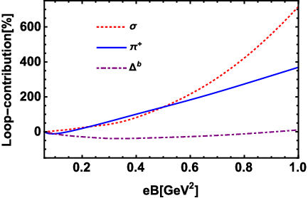
It is observed that except for the charge neutral $\pi^{0}$, which is the only pseudo Goldstone boson of the system preserved by the remnant symmetry of QCD$\times$QED, for all other scalar mesons including the charge neutral $\sigma$, $\pm 1$ charged pseudo scalar $\pi^{\pm}$ and $1/3$ charged scalar diquark $\Delta^{b}$, their masses including the one quark-antiquark loop contribution under magnetic fields are quite different from the point-particle results. We explicitly show the one quark-loop contribution to $\sigma$, $\pi^{\pm}$ and $\Delta^{b}$ as the function of the magnetic field at $T=0,\mu=0$ in Fig.6. The one quark-loop contribution to the charge neutral $\sigma$ and charged $\pi^{\pm}$ increases essentially with the the increase of magnetic fields due to the magnetic catalysis of the polarized quarks. At strong magnetic fields, when $eB>0.5{\rm GeV}^{2}$, the one quark-loop contribution to the mass of charge neutral $\sigma$ meson becomes more essential than the charged $\pi^{\pm}$, and at $eB=1{\rm GeV}^{2}$, the one quark-loop contribution to the mass of charge neutral $\sigma$ meson can reach 8 times of the point-particle results. However, the one quark-quark loop contribution to the scalar diquark mass is negative and less than 50$\%$ of the point-particle result below $eB<0.9{\rm GeV}^{2}$.

References

- [1] J. O. Andersen, W. R. Naylor and A. Tranberg, Rev. Mod. Phys. 88, 025001 (2016) doi:10.1103/RevModPhys.88.025001 [arXiv:1411.7176 [hep-ph]].
- [2] V. A. Miransky and I. A. Shovkovy, Phys. Rept. 576, 1 (2015) doi:10.1016/j.physrep.2015.02.003 [arXiv:1503.00732 [hep-ph]].
- [3] X. G. Huang, Rept. Prog. Phys. 79, no. 7, 076302 (2016) doi:10.1088/0034-4885/79/7/076302 [arXiv:1509.04073 [nucl-th]].
- [4] T. Vachaspati, Phys. Lett. B 265, 258 (1991). doi:10.1016/0370-2693(91)90051-Q
- [5] T. A. Mihara et al., New observations of the cyclotron absorption feature in Hercules X-1,Nature (London)346, 250 (1990); R. C. Duncan and C. Thompson, Astrophys. J. 392, L9 (1992). doi:10.1086/186413; A. Lyne and F. Graham-Smith, Pulsar Astronomy (Cambridge University Press, Cambridge, England, 2005).
- [6] V. Skokov, A. Y. .Illarionov and V. Toneev, Int. J. Mod. Phys. A 24, 5925 (2009).
- [7] W. -T. Deng and X. -G. Huang, Phys. Rev. C 85, 044907 (2012).
- [8] D. Kharzeev and A. Zhitnitsky, Nucl. Phys. A 797, 67 (2007).
- [9] D. E. Kharzeev, L. D. McLerran and H. J. Warringa, Nucl. Phys. A 803, 227 (2008).
- [10] K. Fukushima, D. E. Kharzeev and H. J. Warringa, Phys. Rev. D 78, 074033 (2008).
- [11] S. P. Klevansky and R. H. Lemmer, Phys. Rev. D 39, 3478 (1989). doi:10.1103/PhysRevD.39.3478
- [12] K. G. Klimenko, Theor. Math. Phys. 89, 1161 (1992) [Teor. Mat. Fiz. 89, 211 (1991)]. doi:10.1007/BF01015908
- [13] V. P. Gusynin, V. A. Miransky and I. A. Shovkovy, Nucl. Phys. B 462, 249 (1996) doi:10.1016/0550-3213(96)00021-1 [hep-ph/9509320]; V. P. Gusynin, V. A. Miransky and I. A. Shovkovy, Nucl. Phys. B 563, 361 (1999) doi:10.1016/S0550-3213(99)00573-8 [hep-ph/9908320].
- [14] G. S. Bali, F. Bruckmann, G. Endrodi, Z. Fodor, S. D. Katz, S. Krieg, A. Schafer and K. K. Szabo, JHEP 1202, 044 (2012); G. S. Bali, F. Bruckmann, G. Endrodi, Z. Fodor, S. D. Katz and A. Schafer, Phys. Rev. D 86, 071502 (2012); G. S. Bali, F. Bruckmann, G. Endrodi, F. Gruber and A. Schaefer, arXiv:1303.1328 [hep-lat].
- [15] M. N. Chernodub, Phys. Rev. D 82, 085011 (2010) doi:10.1103/PhysRevD.82.085011 [arXiv:1008.1055 [hep-ph]].
- [16] M. N. Chernodub, Phys. Rev. Lett. 106, 142003 (2011) doi:10.1103/PhysRevLett.106.142003 [arXiv:1101.0117 [hep-ph]].
- [17] N. Callebaut, D. Dudal and H. Verschelde, PoS FACESQCD , 046 (2010) [arXiv:1102.3103 [hep-ph]].
- [18] M. Ammon, J. Erdmenger, P. Kerner and M. Strydom, Phys. Lett. B 706, 94 (2011) doi:10.1016/j.physletb.2011.10.067 [arXiv:1106.4551 [hep-th]].
- [19] Y. Hidaka and A. Yamamoto, Phys. Rev. D 87, no. 9, 094502 (2013) doi:10.1103/PhysRevD.87.094502 [arXiv:1209.0007 [hep-ph]].
- [20] M. Frasca, JHEP 1311, 099 (2013) doi:10.1007/JHEP11(2013)099 [arXiv:1309.3966 [hep-ph]].
- [21] M. A. Andreichikov, B. O. Kerbikov, V. D. Orlovsky and Y. A. Simonov, Phys. Rev. D 87, no. 9, 094029 (2013) doi:10.1103/PhysRevD.87.094029 [arXiv:1304.2533 [hep-ph]].
- [22] Kunlun Wang, PhD thesis from Peking University.
- [23] H. Liu, L. Yu and M. Huang, Phys. Rev. D 91, no. 1, 014017 (2015) doi:10.1103/PhysRevD.91.014017 [arXiv:1408.1318 [hep-ph]].
- [24] H. Liu, L. Yu and M. Huang, Chin. Phys. C 40, no. 2, 023102 (2016) doi:10.1088/1674-1137/40/2/023102 [arXiv:1507.05809 [hep-ph]].
- [25] H. Liu, L. Yu, M. Chernodub and M. Huang, Phys. Rev. D 94, no. 11, 113006 (2016) doi:10.1103/PhysRevD.94.113006 [arXiv:1604.06662 [hep-ph]].
- [26] M. Kawaguchi and S. Matsuzaki, Phys. Rev. D 93, no. 12, 125027 (2016) doi:10.1103/PhysRevD.93.125027 [arXiv:1511.06990 [hep-ph]].
- [27] O. Larina, E. Luschevskaya, O. Kochetkov and O. V. Teryaev, PoS LATTICE 2014, 120 (2014) [arXiv:1411.0730 [hep-lat]].
- [28] E. V. Luschevskaya, O. A. Kochetkov, O. V. Teryaev and O. E. Solovjeva, JETP Lett. 101, no. 10, 674 (2015). doi:10.1134/S0021364015100094
- [29] R. Zhang, W. j. Fu and Y. x. Liu, Eur. Phys. J. C 76, no. 6, 307 (2016) [arXiv:1604.08888 [hep-ph]].
- [30] M. N. Chernodub, Phys. Rev. D 86, 107703 (2012) doi:10.1103/PhysRevD.86.107703 [arXiv:1209.3587 [hep-ph]].
- [31] C. Li and Q. Wang, Phys. Lett. B 721, 141 (2013) doi:10.1016/j.physletb.2013.02.050 [arXiv:1301.7009 [hep-th]].
- [32] M. N. Chernodub, Phys. Rev. D 89, no. 1, 018501 (2014) doi:10.1103/PhysRevD.89.018501 [arXiv:1309.4071 [hep-ph]].
- [33] B. B. Brandt, G. Bali, G. Endr?di and B. Gl?ssle, PoS LATTICE 2015, 265 (2016) [arXiv:1510.03899 [hep-lat]].
- [34] E. V. Luschevskaya, O. E. Solovjeva and O. V. Teryaev, Phys. Lett. B 761, 393 (2016) doi:10.1016/j.physletb.2016.08.054 [arXiv:1511.09316 [hep-lat]].
- [35] S. Fayazbakhsh, S. Sadeghian and N. Sadooghi, Phys. Rev. D 86, 085042 (2012) doi:10.1103/PhysRevD.86.085042 [arXiv:1206.6051 [hep-ph]].
- [36] S. Fayazbakhsh and N. Sadooghi, Phys. Rev. D 88, no. 6, 065030 (2013) doi:10.1103/PhysRevD.88.065030 [arXiv:1306.2098 [hep-ph]].
- [37] S. S. Avancini, W. R. Tavares and M. B. Pinto, Phys. Rev. D 93, no. 1, 014010 (2016) doi:10.1103/PhysRevD.93.014010 [arXiv:1511.06261 [hep-ph]].
- [38] Y. A. Simonov, Phys. Atom. Nucl. 79, no. 3, 455 (2016) [Yad. Fiz. 79, no. 3, 277 (2016)] doi:10.1134/S1063778816030170 [arXiv:1503.06616 [hep-ph]].
- [39] S. S. Avancini, R. L. S. Farias, M. Benghi Pinto, W. R. Tavares and V. S. Tim¨®teo, Phys. Lett. B 767, 247 (2017) doi:10.1016/j.physletb.2017.02.002 [arXiv:1606.05754 [hep-ph]].
- [40] M. Gell-Mann, R. J. Oakes and B. Renner, Phys. Rev. 175, 2195 (1968). doi:10.1103/PhysRev.175.2195
- [41] Y. Nambu and G. Jona-Lasinio, Phys. Rev. 122, 345 (1961).
- [42] Y. Nambu and G. Jona-Lasinio, Phys. Rev. 124, 246 (1961).
- [43] Y. B. He, J. Hufner, S. P. Klevansky and P. Rehberg, Nucl. Phys. A 630, 719 (1998) [nucl-th/9712051].
- [44] P. Rehberg and S. P. Klevansky, Annals Phys. 252, 422 (1996) [hep-ph/9510221].
- [45] S. P. Klevansky, Rev. Mod. Phys. 64, 649 (1992). doi:10.1103/RevModPhys.64.649
- [46] A. Chodos, K. Everding and D. A. Owen, Phys. Rev. D 42 (1990) 2881.
- [47] M. Frasca and M. Ruggieri, Phys. Rev. D 83, 094024 (2011) [arXiv:1103.1194 [hep-ph]].
- [48] N. Ishii, W. Bentz and K. Yazaki, Nucl. Phys. A 587, 617 (1995). doi:10.1016/0375-9474(95)00032-V
- [49] M. Huang, P. f. Zhuang and W. q. Chao, Phys. Rev. D 67, 065015 (2003) doi:10.1103/PhysRevD.67.065015 [hep-ph/0207008].
- [50] M. Huang, Int. J. Mod. Phys. E 14, 675 (2005) [Mod. Phys. Lett. B 14, 675 (2000)] doi:10.1142/S0218301305003491, 10.1142/S0217984900000811 [hep-ph/0409167].
- [51] Z. Wang and P. Zhuang, arXiv:1712.00554 [hep-ph].