Characterization and Efficient Search of Non-Elementary Trapping Sets of LDPC Codes with Applications to Stopping Sets

Consider an undirected graph $G=(F,E)$, where the two sets $F=\{f_{1},\dots,f_{k}\}$ and $E=\{e_{1},\dots,e_{m}\}$, are the sets of nodes and edges of $G$, respectively. We say that an edge $e$ is incident to a node $f$ if $e$ is connected to $f$. If there exists an edge $e_{k}$ which is incident to two distinct nodes $f_{i}$ and $f_{j}$, we represent $e_{k}$ by $f_{i}f_{j}$ or $f_{j}f_{i}$. The degree of a node $f$ is denoted by $d_{f}$, and is defined as the number of edges incident to $f$. The minimum degree of a graph $G$, denoted by $\delta(G)$ is defined to be the minimum degree of its nodes. A node $f$ is called leaf if $d_{f}=1$. A leafless graph $G$ is a graph with $\delta(G)\geq 2$.

Given an undirected graph $G=(F,E)$, a walk between two nodes $f_{1}$ and $f_{k+1}$ is a sequence of nodes and edges $f_{1}$, $e_{1}$, $f_{2}$, $e_{2}$, $\dots$, $f_{k}$, $e_{k}$, $f_{k+1}$, where $e_{i}=f_{i}f_{i+1}$, $\forall i\in[1,k]$. A path is a walk with no repeated nodes or edges, except the first and the last nodes that can be the same. If the first and the last nodes are distinct, we call the path an open path. Otherwise, we call the path a cycle. The length of a walk, a path, or a cycle is the number of its edges. A lollipop walk is a walk $f_{1}$, $e_{1}$, $f_{2}$, $e_{2}$, $\dots$, $f_{k}$, $e_{k}$, $f_{k+1}$, such that all the edges and all the nodes are distinct, except that $f_{k+1}=f_{m}$, for some $m\in(1,k)$. A chord of a cycle is an edge which is not part of the cycle but is incident to two distinct nodes in the cycle. A chordless or simple cycle is a cycle which does not have any chord. The length of the shortest cycle(s) in a graph is called girth, and is denoted by $g$. A graph is called connected when there is a path between every pair of nodes in the graph. A tree is a connected graph that contains no cycles. A rooted tree is a tree in which one specific node is assigned as the root. The depth of a node in a rooted tree is the length of the path from the node to the root. The depth of a tree is the maximum depth of any node in the tree. Depth-one tree (dot) is a tree with depth one.

Any $m\times n$ parity check matrix $H$ of a binary LDPC code $\mathcal{C}$ can be represented by its bipartite Tanner graph $G=(V\cup C,E)$, where $V=\{v_{1},v_{2},\dots,v_{n}\}$ is the set of variable nodes and $C=\{c_{1},c_{2},\dots,c_{m}\}$ is the set of check nodes. If there is an edge $e\in E$ between the nodes $v_{i}$ and $c_{j}$ in the Tanner graph, then, correspondingly, there is a “1” in the $(j,i)$-th entry of matrix $H$. A Tanner graph is called variable-regular with variable degree $d_{\mathrm{v}}$ if $d_{v_{i}}=d_{\mathrm{v}}$, $\forall~{v}_{i}\in V$. A Tanner graph is called irregular if it has multiple variable and check node degrees. An irregular LDPC code is usually described by its variable and check node degree distributions, $\lambda(x)=\sum\limits_{i=d_{v_{\min}}}^{d_{v_{\max}}}\lambda_{i}x^{i-1}$ and $\rho(x)=\sum\limits_{i=d_{c_{\min}}}^{d_{c_{\max}}}\rho_{i}x^{i-1}$, respectively, where $\lambda_{i}$ and $\rho_{i}$ are the fractions of edges in the Tanner graph that are incident to degree-$i$ variable and check nodes, respectively. The terms $d_{v_{\max}},d_{v_{\min}}$ ($d_{c_{\max}},d_{c_{\min}}$) are the maximum and minimum degrees of variable nodes (check nodes), respectively. For variable-regular Tanner graphs, we have $d_{\mathrm{v}}\geq 2$, and for irregular ones, we assume $d_{v_{\min}}\geq 2$. The girth of a Tanner graph is an even number and in this work, we study Tanner graphs that are free of 4-cycles ($g>4$).

For a subset $\mathcal{S}$ of $V$, the subset $\Gamma{(\mathcal{S})}$ of $C$ denotes the set of neighbors of $\mathcal{S}$ in $G$. The induced subgraph of $\mathcal{S}$ in $G$, denoted by $G(\mathcal{S})$, is the graph with the set of nodes $\mathcal{S}\cup\Gamma{(\mathcal{S})}$ and the set of edges $\{f_{i}f_{j}\in E:f_{i}\in\mathcal{S},f_{j}\in\Gamma{(\mathcal{S})}\}$. The set of check nodes with odd and even degrees in $G(\mathcal{S})$ are denoted by $\Gamma_{o}{(\mathcal{S})}$ and $\Gamma_{e}{(\mathcal{S})}$, respectively. In this paper, the terms unsatisfied check nodes and satisfied check nodes are used to refer to the check nodes in $\Gamma_{o}{(\mathcal{S})}$ and $\Gamma_{e}{(\mathcal{S})}$, respectively. The size of an induced subgraph $G(\mathcal{S})$ is defined to be the number of its variable nodes. We assume that an induced subgraph is connected. Disconnected subgraphs can be considered as the union of connected ones.

Given a Tanner graph G, a set $\mathcal{S}\subset V$ is called an (a,b) trapping set (TS) if $|\mathcal{S}|=a$ and $|\Gamma_{o}{(\mathcal{S})}|=b$. Alternatively, $\mathcal{S}$ is said to belong to the class of (a,b) TSs. Parameter $a$ is referred to as the size of the TS. An elementary trapping set (ETS) is a trapping set for which all the check nodes in $G(\mathcal{S})$ have degree 1 or 2. To simplify the representation of ETSs, similar to  [15], [6], [7], we use an alternate graph representation of ETSs, called normal graph in variable-regular graphs. The normal graph of an ETS $\mathcal{S}$ is obtained from $G(\mathcal{S})$ by removing all the check nodes of degree one and their incident edges, and by replacing all the degree-2 check nodes and their two incident edges by a single edge. We call a set $\mathcal{S}\subset V$ an (a,b) leafless ETS (LETS) if $\mathcal{S}$ is an $(a,b)$ ETS and if the normal graph of $\mathcal{S}$ is leafless. Otherwise, the set ${\cal S}$ is called an ETS with leaf (ETSL). A non-elementary trapping set (NETS) is a trapping set which is not elementary. A stopping set (SS) is a trapping set for which $G(\mathcal{S})$ has no check node of degree one. In general, similar to the TSs, SSs can be partitioned into two categories of elementary SSs (ESSs) and non-elementary SSs (NESSs).

The following lemma shows that for variable-regular LDPC codes, depending on $d_{\mathrm{v}}$ being odd or even, some classes of trapping sets cannot exist.

In [7], a hierarchical graph-based expansion approach was proposed to characterize LETSs of variable-regular LDPC codes. It was proved in [7] that any LETS structure of variable-regular Tanner graphs for any variable degree $d_{\mathrm{v}}$, and in any $(a,b)$ class, can be generated by applying a combination of depth-one tree (dot), path and lollipop expansions to simple cycles. Figs. 1 (a)-(c) show the three expansions in the space of normal graphs. (Notations $pa_{m}^{o}$ and $pa_{m}^{c}$ are used for open and closed paths of length $m+1$, respectively. The notation $lo^{c}_{m}$ is used for a lollipop walk of length $m+1$ that consists of a cycle of length $c$.)

The characterization, dubbed as $dpl$, was then used as a road map to devise search algorithms that are provably efficient in finding all the instances of $(a,b)$ LETS structures with $a\leq a_{\max}$ and $b\leq b_{\max}$, for any choice of $a_{\max}$ and $b_{\max}$, in a guaranteed fashion. The $dpl$ search algorithm starts by enumerating short simple cycles in the graph and then searches for the children (descendants) of those cycles through the three expansion techniques recursively, until it reaches the targeted structure.

In [8], LETSs and ETSLs were studied in irregular Tanner graphs. It was shown that these structures in irregular graphs can also be characterized and searched using a $dpl$-based technique in any interest range, efficiently and exhaustively. In the $dpl$ characterization/search algorithm of [7] and [8], to exhaustively cover all the $(a,b)$ LETS structures in the interest range of $a\leq a_{\max}$ and $b\leq b_{\max}$, the algorithm sometimes needs to also cover auxiliary structures with their $b$ values larger than $b_{\max}$, and up to $b^{\prime}_{\max}>b_{\max}$.

To the best of our knowledge, the $dpl$-based algorithms of [7] and [8] are the most efficient exhaustive search algorithms available for finding ETSs of LDPC codes.

The proof of the above result, presented in [9], is based on considering the tree-like expansion of the induced subgraph of the TS starting from the degree-$k$ check node $w$ as the root with $g/2$ layers (depth $g/2-1$). Fig. 2 shows such an expansion. (Variable nodes, satisfied and unsatisfied check nodes are represented by circles, empty and full squares, respectively.)

In this tree, node $w$, in layer one ($L_{1}$), is connected to $k$ variable nodes in layer two ($L_{2}$), and each variable node in $L_{2}$ is connected to $d_{\mathrm{v}}-1$ check nodes in $L_{3}$. Also, to minimize the size of TSs, it is assumed that the degree of all the other check nodes in the subgraph is either $2$ or $1$. From Theorem 1, one can see that for any given values of $b$, $g$ and $d_{\mathrm{v}}$, by increasing $k$, the lower bound on the size of the smallest TS is increased.

It was shown in [9] that the lower bounds of Corollary 1 are often tight. The size of the smallest ETSs was also compared in [9] with the lower bounds of Corollary 1. The following result follows from Table I of [9].

The following lemma is easy to prove based on an approach similar to the one used to prove Theorem 1.

The characterization of ETSs (LETSs and ETSLs) for variable-regular graphs, provided in [7] and [8], is based on normal graph representation of structures. This approach, however, is not applicable to NETSs. In this work, to develop the characterization of NETSs, we investigate the parent-child relationships between ETSs and NETSs. As natural candidates for the expansion of ETSs to reach NETSs, we consider $dot$, $path$ and $lollipop$ expansions. One can see that the application of $path$ and $lollipop$ expansions to a TS increases the $b$ value of the structure rather rapidly. For NETSs with relatively small $b$ values, we thus limit the expansions to $dot$ in the rest of the paper. Due to the low computational complexity of $dot$ expansion [7], this results in an efficient NETS search algorithm starting from ETSs. Using only the $dot$ expansion limits the variety of NETS structures that can be generated starting from ETS structures. In the following, we first discuss the (successive) application(s) of $dot$ expansions to ETS structures and then describe the NETS structures that are out of reach.

Suppose that $\mathcal{S}$ is an $(a,b)$ TS structure of variable-regular Tanner graphs with variable degree $d_{\mathrm{v}}$, where $b\geq 1$. The notation $dot_{m}$ is used for a dot expansion with $m$ edges, connecting a new variable node to $m$ check nodes of $\mathcal{S}$. Similar to [7], we assume that the new variable node in $dot_{m}$ is connected to at least two check nodes of $\mathcal{S}$, i.e., $2\leq m\leq d_{\mathrm{v}}$. However, unlike the $dot_{m}$ used in [7], the $m$ edges can be connected to both satisfied and unsatisfied check nodes of $\mathcal{S}$. The following result is simple to prove.

In the following lemma, we investigate the smallest size of NETS structures with induced subgraphs of the form discussed in Lemma 4 and presented in Fig. 3, for different values of $d_{\mathrm{v}}$, $g$, and $b\leq 4$. Similar results may be derived for other variable degrees, girths and $b$ values.

In the following, we investigate the parent-child relationships between ETSs and NETSs based on $dot_{m}$ expansions. Since the NETS structures discussed in Lemmas 4 and 5 are excluded, in the rest of the paper, we use the expression “interest range of $a$ and $b$” or “$(a,b)$ class of interest” to mean the $b$ values that satisfy $b\leq 4$, and for a given $b$ value in this range, the value of $a$ being strictly less than the entry provided in Table I.

The following corollary describes the exhaustive search of NETSs with only one degree-$3$ check node.

The following result is a generalization of Proposition 2.

Based on the above results, it is easy to see that a NETS structure with $f$ degree-$3$ check nodes can be generated through successive applications of $dot_{m}$ expansions to ETS structures. For this to correspond to an exhaustive search of such NETSs, the following corollary, that generalizes Corollary 2, provides the range of ETSs that need to be included.

The following results can all be proved similar to the cases involving NETSs with only degree-$3$ check nodes. The proofs are thus omitted to avoid redundancy.

Corollaries 2-5 demonstrate that by increasing the multiplicity of check nodes with degrees larger than $2$ and the degrees of such check nodes, the range of $b$ values for ETSs that are needed to provide an exhaustive search of such NETSs is increased. To have an efficient NETS search algorithm based on successive $dot_{m}$ expansions of ETSs, we limit the multiplicity and the degrees of such check nodes to the following cases in the rest of this paper: NETSs containing at most four degree-$3$ check nodes, or containing only one degree-$4$ and at most one degree-$3$ check nodes. We use notations $N_{3},N_{3,3},N_{3,3,3}$, and $N_{3,3,3,3}$, to denote NETS structures with only one up to four check nodes of degree $3$. Notations $N_{4}$ and $N_{4,3}$ are used for NETS structures that contain only one degree-$4$ check node and those with only one degree-$4$ and one degree-$3$ check nodes, respectively.

By restricting the NETS structures to those discussed above, we limit the maximum size $a_{max}$ of NETSs that can be exhaustively covered. The following theorem provides the value of $a_{max}$ for Tanner graphs with different $d_{\mathrm{v}}$ and $g$ values.

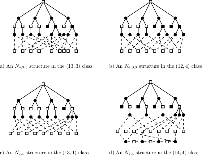
Using Corollary 6, one can find the $b^{\prime}_{\max}$ value which indicates the range of $b$ values for ETSs that are required for the exhaustive search of the desired NETSs. The $b^{\prime}_{\max}$ values for graphs with different $d_{\mathrm{v}}$ values are also provided in Table II. In Table II, we have also included the lower bound on the size of the smallest possible NETS with $b\leq 4$ in brackets. As an example, the entries corresponding to $d_{\mathrm{v}}=3$, and $g=8$ in Table II show that, for such variable-regular graphs, we can exhaustively search all the NETSs with $a=6,7,8,9,10,11$ and $b\leq 4$.

The pseudo-code of the proposed search algorithm is given in Algorithm 1. In the proposed dot-based NETS search algorithm, the input is the exhaustive list of ETSs in the range of $a\leq a_{max}-1$ and $b^{\prime}_{max}$. In the search process, $dot$ expansion is applied to any instance of TSs (ETSs and NETSs) in the interest range of $a\leq a_{max}-1$ and $b\leq b^{\prime}_{max}$. The sets ${\cal I}_{TS}^{a}$ and ${\cal I}_{ETS}^{a}$ are the sets of all the instances of TSs and ETSs in the $(a,b)$ classes with $b\leq b^{\prime}_{\max}$, respectively. The set ${\cal I}_{NETS}^{a}$ is the set of all the instances of NETSs in the $(a,b)$ classes with $b\leq b_{\max}$.

References

- [1] B. k. Butler, and P. H. Siegel, “ Bounds on the minimum distance of punctured quasi-cyclic LDPC codes,” IEEE Trans. Inf. Theory, vol. 59, no. 7, pp. 4584–4597, Jul. 2013.
- [2] A. Dehghan and A. H. Banihashemi, “ On the Tanner graph cycle distribution of random LDPC, random protograph-based LDPC, and random quasi-cyclic LDPC code ensembles,” submitted to IEEE Trans. Inf. Theory, Jan. 2017, available online at: https://arxiv.org/abs/1701.02379
- [3] C. Di, D. Proietti, I. E. Telatar, T. J. Richardson, and R. L. Urbanke,“Finite length analysis of low-density parity-check codes,” in IEEE Trans. Inf. Theory, vol. 48, no. 6, pp. 1570–1579, Jun. 2002.
- [4] M. Esmaeili and M. J. Amoshahy, “On the stopping distance of array code parity-check matrices,” IEEE Trans. Inf. Theory, vol. 55, no. 8, pp. 3488–3493, Aug. 2009.
- [5] H. Falsafain and S.R. Mousavi, “Stopping set elimination by parity-check matrix extension via integer linear programming,” IEEE Trans. Inf. Theory, vol. 63, no. 5, pp. 1533–1540, May. 2015.
- [6] Y. Hashemi and A. Banihashemi, “On characterization and efficient exhaustive search of elementary trapping sets of variable-regular LDPC codes,” IEEE Comm. Lett., vol. 19, pp. 323–326, Mar. 2015.
- [7] Y. Hashemi and A. H. Banihashemi, “New characterization and efficient exhaustive search algorithm for leafless elementary trapping sets of variable-regular LDPC codes,” IEEE Trans. Inf. Theory, vol. 62, no. 12, pp. 6713–6736, Dec. 2016.
- [8] Y. Hashemi and A. H. Banihashemi, “Characterization and efficient exhaustive search algorithm for elementary trapping sets of irregular LDPC codes,” submitted to IEEE Trans. Inf. Theory, Oct. 2016, available online at: http://arxiv.org/abs/1611.10014
- [9] Y. Hashemi and A. H. Banihashemi, “Lower bounds on the size of smallest elementary and non-elementary trapping sets in variable-regular LDPC codes,” to appear in IEEE Comm. Lett., May 2017.
- [10] M. Hirotomo, M. Mohri, and M. Morii, “ On the probabilistic computation algorithm for the minimum-size stopping sets of LDPC codes,” in Proc. IEEE Int. Symp. on Inf. Theory (ISIT), Toronto, Canada, Jul. 2008, pp. 295–299.
- [11] X. Y. Hu, and E. Eleftheriou, “ A probabilistic subspace approach to the minimal stopping set problem,” in Proc. 4th Int. Symp. Turbo Codes and Related Topics, Munich, Germany, Apr. 2006, pp. 295–299.
- [12] X.-Y. Hu, E. Eleftheriou, and D.-M. Arnold, “Regular and irregular progressive edge-growth tanner graphs,” IEEE Trans. Inf. Theory, vol. 51, no. 1, pp. 386–398, Jan. 2005.
- [13] K. M. Krishnan and P. Shankar, “Computing the stopping distance of a Tanner graph is NP-hard,” IEEE Trans. Inf. Theory, vol. 53, no. 6, pp. 2278–2280, Jun. 2007.
- [14] G. B. Kyung and C.-C. Wang, “Finding the exhaustive list of small fully absorbing sets and designing the corresponding low error-floor decoder,” IEEE Trans. Commun., vol. 60, no. 6, pp. 1487–1498, Jun. 2012.
- [15] M. Karimi and A. H. Banihashemi, “On characterization of elementary trapping sets of variable-regular LDPC codes,” IEEE Trans. Inf. Theory, vol. 60, no. 9, pp. 5188–5203, Sep. 2014.
- [16] D. Mackay, “Encyclopedia of sparse graph codes,” URL: http://www.inference.phy.cam.ac.uk/mackay/codes/data.html.
- [17] [Online] Available: http://www.inference.phy.cam.ac.uk/mackay/codes/.
- [18] A. Orlitsky, R. Urbanke, K. Viswanathan, and J. Zhang, “ Stopping sets and the girth of Tanner graphs,” in Proc. Int. Symp. on Inf. Theory (ISIT), Lausanne, Switzerland, Jun./Jul. 2002, pp. 2.
- [19] T. Richardson, “Error floors of LDPC codes,” in Proc. 41th annual Allerton conf. on commun. control and computing, Monticello, IL, USA, Oct. 2003, pp. 1426–1435.
- [20] G. Richter, “Finding small stopping sets in the Tanner graphs of LDPC codes,” in Proc. 41th Int. Symp. on Turbo Codes, Munich, Germany, Apr. 2006, pp. 1–5.
- [21] J. Rosenthal, and P.O. Vontobel “Construction of LDPC codes based on Ramanujan graphs and ideas from Margulis,” in Proc. 38th Annu. Allerton Conf. Commun., Control Comput., Monticello, IL, USA, Oct. 2000, pp. 248–257.
- [22] E. Rosnes and O. Ytrehus, “An efficient algorithm to find all small-size stopping sets of low-density parity-check matrices,” IEEE Trans. Inf. Theory, vol. 55, no. 9, pp. 4167–4178, Sep. 2009.
- [23] E. Rosnes, O. Ytrehus, M. A. Ambroze, and M. Tomlinson, “Addendum to “An efficient algorithm to find all small-size stopping sets of low-density parity-check matrices”,” IEEE Trans. Inf. Theory, vol. 58, no. 1, pp. 164–171, Jan. 2012.
- [24] E. Rosnes, M. A. Ambroze, and M. Tomlinson, “On the minimum/stopping distance of array low-density parity-check codes,” IEEE Trans. Inf. Theory, vol. 60, no. 9, pp. 5204–5214, Sep. 2014.
- [25] J. Stern, “ A method for finding codewords of small weight,” in Coding Theory and Applications, G. Cohen and J. Wolfmann, Eds. New York: Springer-Verlag, 1989, pp.106–113.
- [26] R. M. Tanner, T. D. Sridhara, and T. Fuja, “A class of group-structured LDPC codes,” in Proc. Int. Symp. Commun. Theory Appl., Ambleside, U.K., Jul. 2001, pp. 365–370.
- [27] R. M. Tanner, T. D. Sridhara, A. Sridharan, T. Fuja, and D. Costello, “LDPC block and convolutional codes based on circulant matrices,” IEEE Trans. Inf. Theory, vol. 50, no. 12, pp. 2966–2984, Dec. 2004.
- [28] A. Tasdighi, and A. H. Banihashemi, “Efficient search of girth-optimal QC-LDPC codes,” IEEE Trans. Inf. Theory, vol. 62, no. 4, pp. 1552–1564, Apr. 2016.
- [29] A. Tasdighi, and A. H. Banihashemi, “Symmetrical constructions for regular girth-8 QC-LDPC codes,” IEEE Trans. Commun., vol. 65, no. 1, pp. 14–22, Jan. 2017.
- [30] X. Zhang and P. H. Siegel, “Efficient algorithms to find all small error-prone substructures in LDPC codes,” in Proc. Global Telecommun. Conf., Houston, TX, USA, Dec. 2011, pp. 1–6.
- [31] C.-C. Wang, S. R. Kulkarni, and H. V. Poor, “Finding all small error-prone substructures in LDPC codes,” IEEE Trans. Inf. Theory, vol. 55, no. 5, pp. 1976–1999, May 2009.
- [32] IEEE standard for information technology local and metropolitan area networks specific requirements part 11: wireless LAN medium access control (MAC) and physical layer (PHY) specifications amendment 5: enhancements for higher throughput, IEEE Std. 802.11n-2009, Oct. 29, 2009.
- [33] IEEE standard for local and metropolitan area networks Part 16: air interface for fixed and mobile broadband wireless access systems amendment 2: physical and medium access control layers for combined fixed and mobile operation in licensed bands and corrigendum 1, IEEE Std. 802.16e-2005 and 802.16-2004/Cor 1-2005, Feb. 28, 2006.
- [34] TM Synchronization and Channel Coding. Reston, VA, Consultative Committee for Space Data Systems, Recommended Standard 131.0-B-2, Aug. 2011 [Online]. Available: http://public.ccsds.org/publications/archive/131x0b2ec1.pdf