KEK-TH-2018 RG-improvement of the effective action with multiple mass scales
Abstract
Improving the effective action by the renormalization group (RG) with several mass scales is an important problem in quantum field theories. A method based on the decoupling theorem was proposed in [1] and systematically improved [2] to take threshold effects into account. In this paper, we apply the method to the Higgs-Yukawa model, including wave-function renormalizations, and to a model with two real scalar fields . In the Higgs-Yukawa model, even at one-loop level, Feynman diagrams contain propagators with different mass scales and decoupling scales must be chosen appropriately to absorb threshold corrections. On the other hand, in the two-scalar model, the mass matrix of the scalar fields is a function of their field values and the resultant running couplings obey different RGEs on a different point of the field space. By solving the RGEs, we can obtain the RG improved effective action in the whole region of the scalar fields.
1 Introduction
An effective field theory is a powerful tool to study physics at low energy scale. The standard model (SM) of particle physics is the most successful effective theory in nature that describes physics below TeV scale, from which we can infer physics at higher energy scales. For example, by using the recently observed Higgs boson mass GeV, the running quartic Higgs coupling is shown to decrease as the energy increases. It may either cross zero around GeV, inducing instability of the vacuum, or may asymptotically vanish around the Planck scale, which indicates a possibility that the SM is safely interpolated up to the Planck scale without instability [3, 4, 5, 6, 7, 8, 9]. The behavior of the running quartic coupling is quite sensitive to the precise values of various SM parameters such as the top quark mass or the Higgs mass itself [10, 11, 12]. The importance of is of course related to the shape of the renormalization group (RG) improved effective potential . If there is only a single mass scale , we can safely set the renormalization scale at . However, if there are multiple scales that are different from each other, e.g. , a careful analysis of the effective potential is necessary since a naive choice generates a large logarithm in the effective potential. Such a situation particularly arises when the SM is extended to contain multiple scalar fields 11 1 In the SM itself, since the coupling to the Higgs boson determines its mass, light particles are weakly coupled to the Higgs boson and do not contribute much to the Higgs effective potential. Thus, though SM has multiple hierarchical mass scales, we can safely set the renormalization scale at the heaviest particle mass, i.e. at the top quark mass; the problem of large logarithms is usually not a big issue. The problem becomes important when we extend the SM to contain additional scalar fields that are coupled to the SM..
Suppose that we have multiple scalar fields and that various particles acquire masses through the vacuum expectation values of these scalar fields. At one-loop level in the mass independent scheme, the effective potential is calculated as
| (1) |
where is the tree level potential, and represent the spin and the number of degrees of freedom respectively. are their mass eigenvalues and are the renormalization scales with the scheme dependent constants22 2 For instance, in the scheme, are , and for scalars, fermions and gauge bosons respectively.. If there exists only a single mass scale , we can eliminate the one-loop terms by choosing . Such a choice with the RG-improved couplings corresponds to resumming leading-logarithms to all orders in perturbative calculations [13]. In contrast, if there are several mass scales with very different values, e.g. , a naive choice cannot remove all the large logarithms, and the logarithmic factor such as may invalidate the perturbative calculation.
There are two different but related approaches to handle the issue of multi mass scales: multi-scale renormalization [14, 15] and a decoupling method [1, 17]. In the former approach, several independent renormalization scales are introduced hoping that ’s in Eq.(1) might be replaced by ’s. If such replacements actually occur, all the logarithms can be absorbed by putting . However, as discussed in [15, 16], each RG scale produces a different renormalization group equation (RGE), and it is difficult to solve them keeping the integrability conditions . Furthermore the -functions generically contain logarithms of the ratio of different renormalization scales at higher loops. Thus the perturbative validity will be lost, if there are hierarchical mass scales, e.g. for .
On the other hand, the decoupling method is based on the decoupling theorem in field theories [18, 19]. Below a decoupling scale, massive particles with mass can be integrated out and their effects are absorbed into the effective couplings and higher dimensional operators in the effective field theory of light particles, whose masses are given by a single mass scale denoted by . The radiative corrections in the effective field theory are then given by a single type of logarithms , and consequently we can improve the effective potential by setting The idea is given in [1, 17] and applied to the Higgs-Yukawa model. But in order to avoid large threshold corrections containing , we need to carefully choose the decoupling scale. A systematic procedure to handle such threshold corrections is proposed by [2], in which the authors choose the decoupling scale so that the large logarithms can be absorbed into the effective couplings. The RGEs are constructed in the whole mass scales interpolating below and beyond the decoupling scale.
In this paper, we first generalize the method [2] to include wave function renormalization in the Higgs-Yukawa model, and then apply it to a two real scalar model of with quartic interactions. The mass matix of the scalar fields is a function of , and the mass eigenstates depends on the field values. Thus in order to obtain the RG improved effective potential , we need to use a different RGE on a different point in the field space . Furthermore, because of the scalar mixing, the -functions also depend on the field values. Taking these two effects into account, we can obtain the RG improved effective potential for the two-scalar model. In this paper, we assume that the initial scale of the RGEs starts at a very large scale such as the Planck scale. Of course this is not always necessary, but such a choice helps us to understand the behavior of decoupling as we change (decrease) the renormalization scale .
The paper is organized as follows. In Section 2, we review and generalize the decoupling method [2] in the Higgs-Yukawa model, including the wave function renormalization. The wave function renormalization is given by a diagram containing both of the scalar and the fermion fields in the loop, and their mass scales are generically different. The decoupling method determines the decoupling scale of each term in the effective action so that there are no threshold corrections to the effective coupling. In Section 3, we study a two real scalar model and explicitly calculate the RG improved effective potential. Section 4 is devoted to summary and discussions.
2 Higgs-Yukawa model
In this section, we review the decoupling method of the RG improved effective potential proposed by Casas, Clemente and Quirós [2]33 3 As we mentioned in Introduction, the idea of using the decoupling theorem was first presented in [1]. Based on the idea, the authors of [2] made it clearer how to construct the RGEs which can take into account the threshold effects by carefully introducing the decoupling scales. with a slight generalization to include wave function renormalizations. Let us assume that we have calculated the one-loop effective potential as in Eq.(1). The method adopted by the authors [2] is to replace the ordinary effective potential Eq.(1) by a new one with step functions:
| (2) |
where is a step function which is defined to take 1 (and 0) at higher (lower) energy scale of . When the scale is lower than the largest mass in a one-loop diagram, which we denote , the one-loop correction is set zero by the step function; thus the decoupling of heavy particles can be systematically taken into account. The effective potential is invariant under the RGE if an appropriate wave function normalization is performed. In solving the RGEs, as we see later, the key identity assures absence of further threshold corrections in the low energy effective potential.
In this paper we generalize to consider an effective action in order to study the wave function renormalization as well as renormalization of coupling constants. Suppose we have calculated the effective action;
| (3) |
where and are a tree level and one-loop effective actions respectively. The Feynman diagrams generating the one-loop effective action generally contain various different particles in loops, and denotes a set of particles that are contained in the loop. Applying the method [2], we introduce step functions to incorporate the effect of decouplings;
| (4) |
We have put a prime on the effective action to distinguish it from Eq.(3). Generically contain multiple particles with different mass scales and thus we cannot rewrite the step functions as . One may choose the heaviest mass in the loop diagram as the renormalization scale , but such a choice cannot absorb the threshold corrections in the effective coupling constants unless we expand loop integrals with respect to For example, if two particles with masses, and , exchange in a loop diagram, we will have a Feynman parameter integral such as
| (5) |
If we expanded it with respect to , we would have a simple logarithmic factor with a single mass scale of the heavy field. But it would also generate diverging Feynman parameter integrals,
| (6) |
Thus such an expansion is not justified. Since the integral itself (5) is convergent, we treat the loop integral directly without expanding it with respect to . We will see how to do this explicitly in the Higgs-Yukawa model below.
We now impose the condition that the effective action is invariant under the following RGE;
| (7) |
By solving the RGE (7), we can read the one-loop beta and gamma functions with the decoupling effects of massive particles taken into account. In deriving the RGE, due to the property of , derivatives acting on the step functions vanish;
| (8) |
The absence of the -function terms in the RGE Eq.(7) indicates that further threshold corrections are not generated in solving the equations.
Because of the step functions, the beta and gamma functions jump at the decoupling scales where the step functions jump. It reflects the fact that the threshold corrections in the running couplings are cleverly absorbed in the coupling constants in the low energy effective theory. Such decoupling effects are usually put by hand in the mass independent scheme. The effective action is of course independent of the choice of the renormalization scale , but a convenient one is
| (9) |
All particles are decoupled below the scale and no further radiative corrections arise. As a result, the RG improved effective potential evaluated at the renormalization scale is given by the form of the tree level potential where the coupling constants are replaced by the running couplings calculated by using the beta functions obtained from Eq.(7). The physical meaning of this result is clear. As long as we concentrate on scale lower than the mass of the lightest particle, all the effects of massive particles are absorbed in the effective couplings in the effective theory.
As a simple example, we will show how the RG improvement based on the beta functions derived from Eq.(7) determines the effective action of the Higgs Yukawa model [1]. The action is given by
| (10) |
where is a cosmological constant term, and we have assumed that the fermion does not have a mass term for simplicity. As in [1] and [2], we introduce fermions in order to trace the fermion loops. To calculate the effective action, we expand each field around a classical configuration, , . Then, up to the second order of the fluctuations, the action becomes
| (11) |
where is the classical action, and both of and denote terms quadratic in the fluctuations. Particularly, represents terms proportional to or while contains both fluctuations of the boson and the fermion, and thus induces their mixing. Then, by treating as an interaction term, we get the one-loop effective action as
| (12) |
where we defined the one-loop effective action for a bosonic background, i.e. , by
| (13) |
The total one-loop effective action is then given by
| (14) |
In the following, we simply denote as . After straightforward calculations, we obtain the following one-loop effective action in the scheme:
| (15) |
Here we defined
| (16) |
and
| (17) |
In the calculation we have dropped higher order terms of the derivative expansion. See Appendix for more details of the calculations.
Following the general prescription of Eq.(4), we multiply each term of the effective action by the corresponding step function;
| (18) |
where the step functions are given by
| (19) |
Without loss of generality, we can assume in the following. The integrations over the Feynman parameter in and can be explicitly performed, and we can translate and into step functions with the decoupling scales, and ;
| (20) | ||||
| (21) |
where .
In Fig.1, we plot these decoupling scales as functions of where is fixed to be TeV. They increase as increases and coincide with when it is equal to . For the decoupling scales satisfy , and for . Note that they are well-behaved in the potentially dangerous limits . In the limit,
| (22) |
and in the limit,
| (23) |
They do not coincide exactly with or in the or limit because of the Feynman parameter integral in Eqs.(16)(17): the decoupling scale is a bit smaller than the mass scale of a heavier particle. When one of them is much heavier than the lighter one, the decoupling scale is affected by the presence of the light particle in the loop. Nonetheless the effect is finite. The finiteness is physically natural, but it is not trivial to prove that it is maintained in higher loop corrections. In [2], it was explicitly shown that the decoupling scales appearing in the effective potential are well-behaved up to two loop order. The fact that a heavy particle is not decoupled at the mass but at a lower energy scale will be important in probing physics beyond the SM.
We can now read the one-loop and functions from the RGE Eq.(7);
| (24) | ||||
| (25) | ||||
| (26) | ||||
| (27) | ||||
| (28) |
By solving the running couplings from the above RGEs, we can obtain the improved effective potential. For example, in the region , as far as , both of the boson and the fermion have similar scales of mass . Then both of these fields contribute to the RGEs similarly and decouple around the same energy scale. Therefore, the resultant running couplings at coincide with the ordinary ones that are obtained by solving the usual RGEs without step functions. On the other hand, if , the scalar field is heavier than the fermion and decouples at . Below this scale we have only the fermionic contributions to the RGE. This behavior is schematically shown in the left panel of Fig.2. As a result, the tree-level potential
| (29) |
whose running couplings are evaluated at at each value of coincides with the result in [1].
As shown in Eqs.(24)-(28), the beta and gamma functions are discontinuous at the decoupling scales. Thus the couplings obey different RGEs in each region. However, it can be straightforwardly shown that these seemingly different RGEs describe the same equation and are related by a change of variables. If and is satisfied, the boson is decoupled at higher energy scale and we can expand the bosonic part of the one-loop potential in Eq.(15) with respect to . Then various parameters in the action are modified [1]; 44 4 Note that, in this naive choice of the decoupling scale , we have finite threshold corrections to the coupling constants, e.g. . On the other hand, in our present method, because we define the decoupling scales by the scales where the one-loop corrections vanish, there are no threshold corrections. For example, for the Yukawa term, after the field redefinition , the one-loop correction can be rewritten as which corresponds to the modified coupling constant below the decoupling scales of and . We can obtain the simplified transformation of Eq.(33) by expanding as a function of .
| (30) | ||||
| (31) | ||||
| (32) | ||||
| (33) |
For simplicity, let us assume that the bosonic contributions to the RGEs are all decoupled at the same scale , and denote the beta functions in Eqs.(24)-(28) below (but above as with a prime and those above as without a prime. Then, by using Eqs.(30)-(33), the differential operator defined in Eq.(7) is shown [1] to be identical with the new differential operator ;
| (34) |
More generally, when we distinguish the several decoupling scales, we have seemingly different differential operators in each interval between the decoupling scales. But they all describe the same RGE by the same reasoning above.
The above construction of the improved action is quite general and can be applicable to any field theory with arbitrary number of mass scales. In a theory with only one scalar field, the structure of the improvement is almost the same as the above Higgs-Yukawa model: Introduce step functions in the RGEs and evaluate running couplings at . This gives the RG improved effective action including the threshold corrections. But the construction becomes practically involved in models with multi scalar fields because (i) mass eigenvalues generally depend on several scalar fields and (ii) scalar mixing couplings generate the non-polynomial terms in the effective potential. In the following, we consider a two real scalar model as another example. Such a model is phenomenologically well motivated and it will be important to obtain the RG improved effective action in the whole region of the field values of the two scalars.
3 Two real scalar model
In this section, we calculate the RG improved effective potential of a two real scalar model based on the method presented in the previous section. Since there are no wave function renormalization at one-loop order, we can concentrate on the effective potential. The action is given by
| (35) |
In the following, we denote the tree level potential as . In the scheme, the one-loop effective potential is calculated as
| (36) |
where
| (37) | ||||
| (38) | ||||
| (39) |
In this model, there is no mixture of different particles in a single one-loop diagram and the decoupling scales are simply given by the mass scale of the heavy particle. But there is another complication. As mentioned at the end of the previous section, the effective potential contains a non-polynomial term of the scalar field values through and we need to expand it to obtain polynomial potentials. The one-loop beta functions can be read from the condition that the effective action should be independent on the renormalization scale;
| (40) |
Here we have used the fact that the gamma functions vanish at the one-loop order in the present model. From Eq.(36), the -derivative of is given by
| (41) |
where , and are ordinary one-loop beta functions,
| (42) | ||||
If two mass scales are equal, the second term in Eq.(41) vanishes and we get the ordinary beta functions for . But if there is a hierarchy between these two mass scales, we need to take the effect of in the calculation of the RG improved effective action. By expanding the non-polynomial term and inserting Eq.(41) into Eq.(40), we can obtain the beta functions in which the decoupling effects are automatically taken into account.
Before considering a generic case of , let us first study the case. In this case, there is no scalar mixing and the masses are simply given by
| (43) |
Thus we have
| (44) |
Then, by inserting it into Eq.(40), the beta functions are given by
| (45) |
If we choose the renormalization scale as
| (46) |
we obtain the RG improved effective potential;
| (47) |
The running couplings are evaluated by using Eq.(45). This result agrees with the ordinary RG improved potential, but the RGE itself is different. In the present case, the coupling constants remain at their initial values in the region because of the step functions in Eq.(45). In Fig.3, we plot where is the ordinary improved potential without a step function in . In this figure, we use as the boundary condition of . Then the step function becomes and the decoupling scale is given by . Of course these two effective potentials coincide for . Thus, as long as we take a very high scale such as the Planck scale as an initial scale of RGEs, the present method correctly reproduces the usual improvement in the low energy region .
We now consider a generic case of . We first expand in Eq.(40) as a function of and in order to obtain the beta functions. It is similar to the expansion in the Higgs-Yukawa model which is valid when the condition is satisfied. In the present case, expansions of should be different in different regions of . For example, in a region satisfying , we can expand with respect to . More generally, if we are interested in the effective potential around the following classical configuration (),
| (48) |
we can separate field variables into large and small components by defining new variables as
| (49) |
where Without loss of generality, we can assume that both of the field values or are positive. For the classical configuration Eq.(48), and are satisfied. Thus, around the classical solution, is the large component and we can safely expand with respect to . Substituting and into and expanding it with respect to , we obtain
up to . Using Eq.(49) and inserting it back to Eq.(41), we obtain the beta functions around the classical solution Eq.(48);
| (51) | |||||
| (52) | |||||
| (53) | |||||
These beta functions are different from the ordinary ones Eq.(42) when because the decoupled component with mass is different for a different value of . The second terms in the beta functions represent the effects of the lighter particles with mass , and contribute to the RGEs during the scale . Note that the coefficients of the second terms depend on .
In Fig.4, we show the second terms in the beta functions as functions of , normalized by the first terms, i.e. the ordinary beta functions Eq.(42). As we saw in Fig.4, the effect can be sizable if there is a large hierarchy between the two mass scales. For example, suppose and for simplicity. Along the direction , we have
| (54) |
If , we have . Hence, if we take the Planck scale as the initial scale of the RGE and at the EW scale GeV, gives a typical order of corrections to the low energy effective couplings below the EW scale due the step functions in the beta functions. Here denotes the coefficient of in the beta function Eq.(52). Thus the ratio of the decoupling effect to the total change of the effective coupling
| (55) |
becomes sizable if and .
In the upper left panel of Fig.5, we show the running couplings obtained from Eqs.(51)-(53) in the direction . Here, all the dimensional quantities are normalized by the initial value of the initial renormalization scale . We can see the step behaviors, particularly in , corresponding to the step functions in the beta functions. In the upper right panel of Fig.5, we show the running couplings as a function of by putting . Note that, when becomes sufficiently large so that is larger than , all the couplings stop running because all the particles are decoupled. By using these running couplings, the improved effective potential is given by
| (56) |
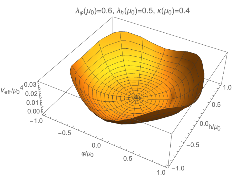
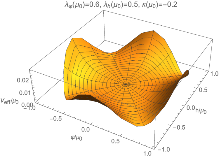
In the lower panel in Fig.5, we show a result of our numerical calculation. Here, is fixed to be zero and the potential is normalized by its tree-level one without any improvement. As we mentioned before, this ratio becomes one in the region because all the particles decouple and there is no running effects. By changing and , one can obtain the improved effective potential in the whole region of , and it is shown in Fig.6. Here, the left (right) panel corresponds to the case.
4 Summary and Discussions
In this paper, we studied RG improvement of the effective action of a Higgs-Yukawa model and a two real scalar model based on the decoupling approach [2]. In this approach, the RGEs can automatically take into account decouplings of massive particles and their threshold corrections by introducing appropriately chosen step functions. In models with multiple scalar fields, the mass matrix is a function of field values, and decoupling scales of heavy particles depend on them. As a result, we need to use a different RGE on each point of the field space. Furthermore, because of the scalar mixing, the effective potential generally has non-polynomial terms. By expanding them, we also get field-dependent -functions. Taking these effects into account, we have obtained the RG improved effective potential for the two real scalar model. If there is a large hierarchy between multiple mass scales, the effect might be sizable. We also investigated decoupling scales when various fields with different masses simultaneously exchange in a loop diagram. A simple example is the one-loop wave function renormalization in the Higgs-Yukawa model. Since both of heavy and light fields contribute to the diagrams, the decoupling scales are given by neither of their masses but complicated combinations of them.
We now comment on an extension of the method to higher loop corrections. In [2], the authors proposed a generalization to 2-loop diagrams and showed that the decoupling scales are well-behaved in potentially dangerous limits where multiple mass scales have infinitely large hierarchy or . A key identity here is , where is the operator defined in Eq.(7). Suppose that the model has a loop expansion parameter . Then the effective action is written up to -th loop as
| (57) |
where is the classical action and are -th loop contributions to the effective action which can be further decomposed as Here denotes both of differences of operators, namely etc. and differences of Feynman diagrams. terms determines the beta and gamma functions. Namely the invariance of the effective action under a change of renormalization scale relates terms for with the terms. In order to define the effective action with step functions as in (4), it is necessary to respect the relations between various different terms. One possibility will be to introduce a different step function in each diagram with as we did in the Higgs-Yukawa model for one-loop calculations, and determine the step functions for terms so as to respect the RG relations, but since the logarithmic structures of higher loop diagrams are complicated, more detailed studies will be necessary. We leave it for future investigations. This prescription is slightly different from the 2-loop prescription proposed by [2]. In their prescription, logarithmic terms are expanded with respect to where is the largest mass scale in the model. Here the question is whether we can reduce various logarithms including multiple mass scales such as into those with a single mass, . As we saw in the Higgs-Yukawa model, in order to avoid divergences of Feynman parameter integrals, we need to treat logarithmic factors in loop integrals without using an expansion with respect to . Thus the decoupling scales are not simply given by a single heavy mass, but a complicated combination of various masses. In the case of and in Eq.(19) of the Higgs-Yukawa model, they are in between the heavy and the light mass scales and monotonically increase as the heavy mass becomes larger as in Fig.1. They are also well-behaved in the potentially dangerous limit; . These behaviors are also expected to hold even for higher loop effects. We want to come back to these problems in future.
Acknowledgements
This work of SI is supported in part by Grants-in-Aid for Scientific Research (No. 16K05329) from the Japan Society for the Promotion of Science. The work of KK is supported by the Grant-in-Aid for JSPS Research Fellow, Grant Number 17J03848.
Appendix: One-loop calculations of Higgs-Yukawa model
In this appendix, we give the derivation of Eq.(15). First, let us consider the effective action in the bosonic background;
| (58) |
The first term of the right hand side corresponds to the scalar contributions to the one-loop effective potential. The second term of the fermionic contributions can be rewritten as
| (59) |
where we have used the fact that the action is invariant under . Then, by expanding the second term of Eq.(59) with respect to , we obtain
| (60) |
where . This term gives the wave function renormalization in the RGE.
Next, let us consider the fermionic background, i.e. the third term of the right hand side of Eq.(14). For our present purpose, it is sufficient to consider a constant . By expanding the logarithm, we have
| (61) |
Then, by introducing a relative coordinate and expanding with respect to , we obtain
| (62) |
where we have used the following identity:
| (63) |
The first term in Eq.(62) gives the one-loop correction to the Yukawa term:
| (64) |
The second term of Eq.(62) gives the one-loop correction to the kinetic term of :
| (65) |
References
- [1] M. Bando, T. Kugo, N. Maekawa and H. Nakano, “Improving the effective potential: Multimass scale case,” Prog. Theor. Phys. 90, 405 (1993) doi:10.1143/PTP.90.405, 10.1143/ptp/90.2.405 [hep-ph/9210229].
- [2] J. A. Casas, V. Di Clemente and M. Quiros, “The Effective potential in the presence of several mass scales,” Nucl. Phys. B 553, 511 (1999) doi:10.1016/S0550-3213(99)00262-X [hep-ph/9809275].
- [3] M. Holthausen, K. S. Lim and M. Lindner, “Planck scale Boundary Conditions and the Higgs Mass,” JHEP 1202, 037 (2012) doi:10.1007/JHEP02(2012)037 [arXiv:1112.2415 [hep-ph]].
- [4] F. Bezrukov, M. Y. Kalmykov, B. A. Kniehl and M. Shaposhnikov, “Higgs Boson Mass and New Physics,” JHEP 1210, 140 (2012) doi:10.1007/JHEP10(2012)140 [arXiv:1205.2893 [hep-ph]].
- [5] G. Degrassi, S. Di Vita, J. Elias-Miro, J. R. Espinosa, G. F. Giudice, G. Isidori and A. Strumia, “Higgs mass and vacuum stability in the Standard Model at NNLO,” JHEP 1208, 098 (2012) doi:10.1007/JHEP08(2012)098 [arXiv:1205.6497 [hep-ph]].
- [6] S. Iso and Y. Orikasa, “TeV Scale B-L model with a flat Higgs potential at the Planck scale - in view of the hierarchy problem -,” PTEP 2013, 023B08 (2013) doi:10.1093/ptep/pts099 [arXiv:1210.2848 [hep-ph]].
- [7] D. Buttazzo, G. Degrassi, P. P. Giardino, G. F. Giudice, F. Sala, A. Salvio and A. Strumia, “Investigating the near-criticality of the Higgs boson,” JHEP 1312, 089 (2013) doi:10.1007/JHEP12(2013)089 [arXiv:1307.3536 [hep-ph]].
- [8] K. Kawana, “Criticality and inflation of the gauged B – L model,” PTEP 2015, 073B04 (2015) doi:10.1093/ptep/ptv093 [arXiv:1501.04482 [hep-ph]].
- [9] Y. Hamada and K. Kawana, “Vanishing Higgs Potential in Minimal Dark Matter Models,” Phys. Lett. B 751, 164 (2015) doi:10.1016/j.physletb.2015.10.006 [arXiv:1506.06553 [hep-ph]].
- [10] S. Alekhin, A. Djouadi and S. Moch, “The top quark and Higgs boson masses and the stability of the electroweak vacuum,” Phys. Lett. B 716, 214 (2012) doi:10.1016/j.physletb.2012.08.024 [arXiv:1207.0980 [hep-ph]].
- [11] S. Moch et al., “High precision fundamental constants at the TeV scale,” arXiv:1405.4781 [hep-ph].
- [12] G. Cortiana, “Top-quark mass measurements: review and perspectives,” Rev. Phys. 1, 60 (2016) doi:10.1016/j.revip.2016.04.001 [arXiv:1510.04483 [hep-ex]].
- [13] S. R. Coleman and E. J. Weinberg, “Radiative Corrections as the Origin of Spontaneous Symmetry Breaking,” Phys. Rev. D 7, 1888 (1973). doi:10.1103/PhysRevD.7.1888
- [14] M. B. Einhorn and D. R. T. Jones, “A New Renormalization Group Approach To Multiscale Problems,” Nucl. Phys. B 230, 261 (1984). doi:10.1016/0550-3213(84)90127-5
- [15] C. Ford and C. Wiesendanger, “Multiscale renormalization,” Phys. Lett. B 398, 342 (1997) doi:10.1016/S0370-2693(97)00237-2 [hep-th/9612193].
- [16] T. G. Steele, Z. W. Wang and D. G. C. McKeon, “Multiscale renormalization group methods for effective potentials with multiple scalar fields,” Phys. Rev. D 90, no. 10, 105012 (2014) doi:10.1103/PhysRevD.90.105012 [arXiv:1409.3489 [hep-ph]].
- [17] M. Bando, T. Kugo, N. Maekawa and H. Nakano, “Improving the effective potential,” Phys. Lett. B 301, 83 (1993) doi:10.1016/0370-2693(93)90725-W [hep-ph/9210228].
- [18] T. Appelquist and J. Carazzone, “Infrared Singularities and Massive Fields,” Phys. Rev. D 11, 2856 (1975). doi:10.1103/PhysRevD.11.2856
- [19] K. Symanzik, “Infrared singularities and small distance behavior analysis,” Commun. Math. Phys. 34, 7 (1973). doi:10.1007/BF01646540