Università degli Studi di Napoli “Federico II”
\facultyScuola Politecnica e delle Scienze di Base
Dipartimento di Fisica “Ettore Pancini”
\logologo.eps
\courseFisica
\degreeyear2016/2017
\chairProf. Giampiero Esposito
\numberofmembers1
\matrnumN94000312
Asymptotic Structure and
Bondi-Metzner-Sachs group in General Relativity
Introduction
In this work the asymptotic structure of space-time and the main properties of the Bondi-Metzner-Sachs (BMS) group, which is the asymptotic symmetry group of asymptotically flat space-times, are analysed. Every chapter, except the fourth, begins with a brief summary of the topics that will be dealt through it and an introduction to the main concepts. The work can be divided into three principal parts.
The first part includes the first two chapters and is devoted to the development of the mathematical tools that will be used throughout all of the work. In particular we will introduce the notion of space-time and will review the main features of what is referred to as its causal structure and the spinor formalism, which is fundamental in the understanding of the asymptotic properties.
In the second part, which includes the third, fourth and fifth chapters, the topological and geometrical properties of null infinity, , and the behaviour of the fields in its neighbourhood will be studied. Particular attention will be paid to the peeling property.
The last part is completely dedicated to the BMS group. We will solve the asymptotic Killing equations and find the generators of the group, discuss its group structure and Lie algebra and eventually try to obtain the Poincaré group as its normal subgroup.
The work ends with a brief conclusion in which are reviewed the main modern applications of the BMS group.
Chapter 1 Causal Structure
Abstract
In this first chapter we analyse what is referred to as the causal structure of the space-time. In particular we will start by giving, in the first section, the definition of a space-time, that will be used throughout all of the work. In the other sections the notions of orientability and causality, i.e. chronological and causal past and future sets and their topological properties, will be considered. Having defined these concepts, from section 1.6 we will start to explore the meaning of ‘causality-violating’ space-time and to take into account the restrictions to impose on a space-time for it to be ‘physical’. The last section is devoted to the global hyperbolicity and the existence of Cauchy surfaces and will be very important to discuss the asymptotic properties, which are subjects of the last chapters.
The main bibliography for this chapter is furnished by the beautiful works of Penrose, Hawking and Geroch.
1.1 Introduction
The mathematical model we shall use for the description of space-time, i.e. the collection of all events, is a four-dimensional manifold (see Appendix A for definitions). In fact a manifold corresponds naturally to our intuitive ideas of the continuity of space and time. So far this continuity is thought to be valid for distances greater than a certain cut-off of about cm (the Planck length) and actually has been established for distances down to cm by experiments on pion scattering. For the description of phenomena that occur at distances lesser than this cutoff our model for space-time could become inappropriate and other different structures may emerge, due to quantum effects. It is worth remarking that the first physicist who introduced the Planck scale value was the Soviet theoretical physicist Matvei Petrovich Bronstein in his work ‘Quantization of Gravitational Waves’ of 1936 in which he analysed the problem of the measurability of the gravitational field. He calculated the “absolute minimum for the indeterminacy” in the weak-field framework and formulated the following conclusion:
“The elimination of the logical inconsistencies connected with this requires a radical reconstruction of the theory, and in particular, the rejection of a Riemannian geometry dealing, as we have seen here, with values unobservable in principle, and perhaps also the rejection of our ordinary concepts of space and time, replacing them by some much deeper and non-evident concepts.”
(Bronstein, 1936)
In such a way, the quantum limits of General Relativity were revealed for the first time.
Before investigating the causal structure of space-time, which explores the causal relationships between the events,
we will start by asking the question “What is the underlying manifold of our universe?”. To answer we need to make some physical and reasonable assumptions.
The first consideration is that no ‘edges’ of the universe have ever been observed. The edges can be mathematically represented by boundaries and hence we assume to have no such boundaries. Furthermore we take to be a connected Hausdorff manifold. In fact we don’t have knowledge of any disconnected components and moreover there could not be any communication between separated connected components of our universe. The Hausdorff condition says that any pair of points can be separated by disjoint neighbourhoods. Thus violating Hausdorff condition would imply a violation of concept of ‘distinct events’.
We know that General Relativity requires more than merely a manifold: there must be a metric tensor field defined over it that possesses a Lorentz signature. The following theorem is remarkable.
Theorem 1.1.1.
(Geroch, 1968) Let be a connected, Hausdorff 4-manifold with a Lorentzian metric tensor . Then the topology of has a countable basis.
Thus we may infer that is paracompact, according to A.0.6. This property, physically, prevents a manifold from ‘being too large’. Paracompatness has a number of important consequences. It can be shown that paracompactness implies that all connected components of can be covered by a countable family of charts and that there exists a partition of unity which allows us to define a Riemannian metric over as discussed in Appendix A (see (A.0.1), A.0.5 and (A.0.2)).
The order of differentiability, , of the metric must be sufficient for the field equation to be defined. Those equations, involving the metric tensor components , can be defined in a distributional sense if and its inverse are continuous and have locally square integrable generalized first derivatives with respect to the coordinate system. But this condition is not sufficient, since it guarantees neither the existence nor the uniqueness of geodesics, for which a metric is required. In the remainder we will simply assume the metric to be because probably the order of differentiability of the metric is not physically relevant. In fact, since one can never measure the metric exactly, but only with some margin of error, one could never determine that there is an actual discontinuity in its derivatives of any order. Thus we are led to this definition of space-time:
Definition 1.1.1.
A space-time is a real, four-dimensional connected Hausdorff manifold without boundary with a globally defined tensor field of type , which is non-degenerate and Lorentzian. By Lorentzian is meant that for any there is a basis in (the tangent space to at ) relative to which is represented by the matrix .
Remark 1.1.1.
Two space-times and will be taken to be equivalent if there is a diffeomorphism which carries the metric into the metric , i.e. . So it would be more correct to define the space-time to be the equivalence class of , two space-times being equivalent if their metrics are linked by a diffeomorphism. However we will work with just one representative member of the above mentioned equivalence class.
1.2 Orientability
The presence of the metric tensor enables us to give the following
Definition 1.2.1.
Let be a space-time, with . Then any tangent vector is said to be: timelike, spacelike or null according as (summation over the repeated indices, according to Einstein’s convention) is positive, negative or zero.
The null cone at is the set of null vectors in . The null cone in disconnects the timelike vectors into two separate components, the future-directed one and the past-directed one. Similarly, the set of all triads of unit, mutually orthogonal, spacelike vectors at can be divided into two classes, which could be designated the left-handed and right-handed triads.
Physically the designation of future- and past-directed timelike vectors corresponds to a choice of a direction for the arrow of time, while the designation of left- and right-handed triads to a choice of spatial parity. Those choices can be made at each point of . We may ask whether or not such designations can be made globally over the entire . Then we are led to the following
Definition 1.2.2.
A space-time is said to be time-orientable if a designation of which timelike vectors are to be future-directed and which past-directed can be made at each of its point, where this designation is continuous from point to point over the entire manifold .
Each of these two designations is called a time-orientation. A similar definition holds for space-orientability and space-orientation, involving the triads mentioned above.
A space-time is clearly time-orientable if there exists a nowhere vanishing timelike vector field, i.e. one can choose at each point one of the two oppositely directed unit timelike vectors along a given direction, this choice being continuous from point to point. Conversely, since a space-time is paracompact, there exists a smooth Riemannian metric defined on . Thus at there will be a unique future-directed timelike vector that can be chosen to be the unit eigenvector with positive eigenvalue , of with respect to , i.e. , . Thus we have obtained the following
Proposition 1.2.1.
A space-time is time-orientable if and only if there exists a smooth non-vanishing timelike vector field on .
The above definitions of orientability are not in general the most useful. Fortunately there is a much simpler characterization, that is given below.
Consider a space-time , and fix a point . Consider then a closed curve beginning and ending at . We can fix a time-orientation at and carry this choice continuously about from point to point, until we revert to , and thus have a final orientation which will be either the same or the opposite as with which we began, according to the fact that is time-preserving or time-reversing. Then by definition of time-orientability we have that is time-orientable if any closed curve through each of its point is time-preserving. We can easily show the converse. Consider again a point and choose there a time-orientation. Then choose a time-orientation at any other point by carrying the choice made at continuously along some curve joining and . The resulting time-orientation at will be unambiguous: in fact, given another curve joining and , it can be combined with the original to obtain a closed curve through , that has to be, by hypothesis, time-preserving. Thus, repeating this procedure for every point of we can obtain in each of them a definite time-orientation. We can conclude that
Proposition 1.2.2.
A space-time is time-orientable if and only if every closed curve through each of its points is time-preserving.
Again, the same argument can be carried out for space-orientability.
Thus, in order to decide whether or not a space-time is time orientable one has only to ‘test’ time-orientation about all the closed curves through a given point . However the number of curves to test can be reduced considerably, as will be shown. We call two closed curves, and through homotopic if can be continuously deformed into , i.e. if there exists a 1-parameter family of curves, , with the parameter varying in , such that and . For example any two closed curves through the origin in the plane are homotopic, while a closed curve on the annulus that wraps around the hole is not homotopic to one which does not. Since a continuous deformation cannot result in the discontinuous change from time-preserving to time-reversing, two closed homotopic curves are both time-preserving or time-reversing. Then we just need to evaluate the time-orientation of curves belonging to different homotopy equivalence classes.
Definition 1.2.3.
A manifold is simply connected if any two closed curves through any are homotopic.
Then we have
Proposition 1.2.3.
Every space-time based on a simply connected manifold is both time- and space-orientable.
We illustrate now what are the appropriate orientation properties of a ‘physically’ realistic model of our universe. Consider a space-time and fix a point . Each point of defines several points of a new space-time, , as follows. Consider pairs , where is a point of and a generic curve in from to . Two of such pairs and are called equivalent if and and are homotopic, and we say . We define to be the set of the just defined equivalence classes, i.e. . Thus, a point of is just a point of and a curve from to that point, up to a continuous deformation of the curve. We build the metric defining the distance between two points and of just as the distance between and in . The resulting space-time is called universal covering space-time of . The two space-times are locally indistinguishable, but globally they are not. In fact if we suppose to be simply connected then only provided that . In this case the universal covering will be identical to the original space-time. To each point of there corresponds just one point of . But if we take to be, for example, the two dimensional annulus (which is not simply connected), as shown in figure (1.1), then for the point in the curve can be continuously deformed into , , and hence the two pairs define the same point on , but it cannot be deformed continuously into which winds one time around the hole, is not equivalent to and the two pairs define different points in . More generally a curve which reaches from after winding around the hole times will be deformable to a curve which winds around the hole the same number of times. Each point of , therefore, will give rise to an infinite number of points of , one for each value of the integer .

As shown in figure 1.1 we have just unwrapped the annulus. Universal covering space-times of any space-time are always simply connected and therefore always time- and space-orientable. Their importance is related to the fact that they are physically indistinguishable form the original space-time because the only effect of taking the universal covering space-times is to produce possibly several copies of each local region in the original one, leaving the ‘local physics’ unaffected. The conclusion is that no physical possibilities would be lost by demanding that one space-time should be time- or space-orientable. We can eventually state the following
Proposition 1.2.4.
If a space-time is not simply connected (and hence not time-orientable), there always exists a simply connected (and hence time-orientable) space-time , which is its universal covering.
1.3 The Exponential Map
To proceed further we shall need some simple properties of the exponential map. Here and in the remainder we will assume the presence of a , torsion-free connection on the space-time . For any , the exponential map is a smooth () map from some open subset of the tangent space , into
such that the affinely parametrized geodesic with tangent vector at and parameter value at acquires the parameter value at . This map is not defined for all , since a geodesic may not be defined for all . If takes all values the geodesic is said to be a complete geodesic. The manifold is said to be geodesically complete if all geodesics on are complete, i.e. maps the whole into for every . That means that every affinely parametrized geodesic in extends to arbitrarily large parameter values. But whether is complete or not, it may well be that several different elements of are mapped to the same point of , as shown in Figure 1.2, or that the map is badly behaved for certain elements of (because its jacobian vanishes).


We require for the present that, for each there is some open neighbourhood of the origin in and an open neighbourhood of in such that is a diffeomorphism from to . Such a neighbourhood is called normal neighbourhood of . Furthermore, one can choose to be convex, i.e. to be such that any point in can be joined to any other point in by a unique geodesic starting at and totally contained in . Within a normal neighbourhood one can define coordinates by choosing any point , choosing a basis of , and defining the coordinate of the point by the relation . In this way one assigns to the coordinates, with respect to the basis , of the point in . Then and . Such coordinates will be called normal coordinates based on .
1.4 Chronology and Causality
Let be a space-time with fixed time-orientation and and any two points of .
Definition 1.4.1.
The point chronologically precedes , , if there exists a future-directed timelike curve (i.e. whose tangent vector is timelike future-directed) with past endpoint and future endpoint .
The ‘precedes’ relation is the central one of what is called the causal structure of space-time. Physically it means that the events represented by and are causally related, in the sense that a signal can be sent from to be received later from .
We have immediately the following
Theorem 1.4.1.
If and then .
Proof.
It is sufficient to draw the timelike curves and , that must exist by hypothesis and joining them at . Their union, is a union of timelike curves, and hence timelike, which connects and . Thus . ∎
Definition 1.4.2.
- •
The set is called the chronological past of ;
- •
The set is called the chronological future of ;
- •
Given a subset the set is called the chronological past of ;
- •
Given a subset the set is called the chronological future of .
Since one can always perform a sufficiently small deformation of a timelike curve while preserving the timelike nature of the curve, it follows that for all there exists an open neighbourhood of such that . Thus
Proposition 1.4.1.
is an open subset of , for every .
The same property holds for , being the union of open sets.
As an example, in Minkowski space-time with the usual coordinates , if then and are just the interiors of the past and future light-cones of .
Definition 1.4.3.
The point causally precedes , , if there exists a future-directed causal curve (i.e. whose tangent vector is timelike or null future-directed) with past endpoint and future endpoint .
Remark 1.4.1.
Note that Penrose (1972b) defines the chronologically and causally precedes relations using not arbitrary timelike and null curves, but geodesics which are easier to handle mathematically.
We have similar definitions for the causal past of , and for the causal future of , . In the remainder, to show the topological properties of the above defined sets, we will only use the future ones, being clear that they are valid for the past ones too.
In the above example of Minkowski space-time we have and , these sets being closed, and furthermore we have that the boundaries of are generated by the null geodesics starting from . However neither of this last properties is valid in general. We can immediately give an example of space-time in which is not closed and where are not generated by null geodesics starting from . Let be a space-time and consider a closed subset of . Then with the metric induced by is, if connected, itself a space-time (that be closed was necessary to ensure that even be a manifold). This simple argument allows us to buil a new space-time from a given one, by, for example, removing a point of it. If now we consider Minkowski space-time with one point removed, as shown in Figure 1.3, then is not closed since the null geodesic beyond the removed point, which extends from , is not part of whereas it is part of .

Anyway the two properties mentioned above remain valid locally, as stated by the following
Theorem 1.4.2.
Let be an arbitrary space-time and let . Then there exists a convex normal neighbourhood of
Furthermore, for any such , , i.e. the chronological future of in the space-time , consists of all points reached by future-directed timelike geodesics starting from and contained within , and has its boundary generated by future-directed null geodesics in starting from .
The proof of the first proposition can be found in (Hicks, 1965, pg. 32) while the second in (Hawking and Ellis, 1973, pg. 103).
Let and be a causal curve beginning at and ending at . Since is a compact subset of (being the continuous image of a closed interval) it can be covered by a finite number of convex normal neighbourhoods , as shown in Figure 1.4.

If failed to be a null geodesic in any such neighbourhood, then, using Theorem 1.4.2 we can always deform into a timelike geodesic in that neighbourhood and then extend this deformation to the other neighbourhoods to obtain a timelike curve from to , call it . Thus we have the following
Corollary 1.4.1.
If , then any causal curve connecting to must be a null geodesic.
Sometimes the set is called the future horismos of .
Since for any set it can be shown that and clearly , it follows immediately that
Similarly we have and hence
1.5 Pasts, Futures and Achronal Boundaries
From 1.4.2 we saw that the boundary of or is formed, at least locally, by the future-directed null geodesics starting from . To derive the properties of more general boundaries we introduce the concepts of achronal and future sets.
Definition 1.5.1.
A set is said to be an achronal set if , i.e. if no two points of are chronologically related.
Note that a set can be locally spacelike without being achronal, as shown in Figure 1.5. Examples of achronal sets are the future light cone in Minkowski space-time, , the null hyperplane and the spacelike plane .

Definition 1.5.2.
A set is said to be future set if for some set .
By proposition 1.4.1 a future set is always open.
Definition 1.5.3.
If is a future set, its boundary is called achronal boundary, i.e. .
The next theorem asserts that the boundary of the future of a set, the above defined achronal boundary, even if does not need to be smooth, always forms a ‘well behaved’, 3-dimensional, achronal surface.
Theorem 1.5.1.
Let be a space-time and let be a future set for , . Then the achronal boundary is an achronal, 3-dimensional, embedded topological submanifold of .
Proof.
Let . If , then and since is open, an open neighbourhood of is contained in (see Figure 1.6). We have , being on . Thus we have . In particular . By following the same argument we have . If failed to be achronal we could find two points in it, say and , such that , and hence , by the previous result. However, this is impossible since is open and there is no point lying both in and . Thus is achronal.

To obtain the manifold structure of we introduce normal coordinates in a neighbourhood of such that is timelike in and that the integral curves of , enter and . But this implies that each such curve intersects , and since is achronal, it must intersect it at precisely one point (otherwise we would obtain two or more points joined by a timelike curve).

Thus in each such neighbourhood, we get a one-to-one association of points of with the coordinates characterizing the integral curve of , i.e. defined by () for . Furthermore the value of at the intersection point must be a function of the coordinates and thus the map is a homomorphism. Since this construction can be repeated for all we obtain a collection that is a atlas for , which makes it an embedded topological manifold. ∎
For the purpose of what follows we need to introduce several definitions that will play an important role. First, it will be convenient to extend the definition of timelike and causal curve from piecewise differentiable to continuous, it being essential in taking limits.
Definition 1.5.4.
A continuous curve , where is an interval of , is future-directed causal if for every , there is a neighbourhood of in and a convex normal neighbourhood of in such that for any , if and if .

The same definition holds for timelike curve, with replacing . The sense of the definition is that, for a continuous curve, locally, pairs of points on the curve can be joined by a differentiable timelike or causal curve. Note that the timelike or causal nature of the curve is left unchanged by a continuous, one-to-one, reparametrization, and hence two curves which differ by such a reparametrization will be considered equivalent.
Next we need the notion of extendibility of a curve, and hence we give before the definition of endpoint of a non-spacelike curve.
Definition 1.5.5.
A point will be said to be future endpoint of a future-directed causal curve if for every neighbourhood of there is a such that for every .
Note that the endpoint need not lie on the curve, i.e. there need not exist a value of such that . This allows us to give the following
Definition 1.5.6.
A causal curve is future-inextendible if it has no future endpoint.
A similar definition holds for past-inextendibility.
We give now the definition of convergence of causal curves.
Definition 1.5.7.
Let be an infinite sequence of causal curves.
- •
A point will be said to be a convergence point of if, given any open neighbourhood of p, there exists an such that for all .
- •
A curve will be said to be a convergence curve of if each is a convergence point.
- •
A point will be said to be a limit point of if every open neighbourhood of intersects infinitely many .
- •
A curve will be said to be the limit curve of if there exists a subsequence for which is a convergence curve.
The previous definitions allow us to state and prove the following
Theorem 1.5.2.
Let be an open set and be an infinite sequence of causal curves which are future-inextendible with limit point . Then through there is a causal curve which is future-inextendible and which is a limit curve of .
Proof.
Let be a convex normal coordinate neighbourhood about and let be the open ball of coordinate radius with center . Let be a subsequence of which converges to . Since the sphere is compact it will contain the limit point of the , the latter being a subsequence. Any such limit point must lie either in or because of the causal nature of the curves. Choose
| (1.5.1) |
to be one of these limit points, and choose to be a subsequence of which converges to . We can continue inductively, defining
as a limit point of the subsequence for , for and , and defining as a subsequence of the above subsequence which converges to .

For example the point , situated on is a limit point of and a convergence point of . We are just constructing, in turn, all the coordinate spheres whose radii are rational multiples, between and of and continuing to extract limit points lying on these spheres and subsequences converging to these points. Since any two of the will have a causal separation, the closure of the union of all the will give a causal curve from to . To show that is a limit curve of we have to construct a subsequence of the such that for each , converges to . We choose to be a member which intersects each of the balls for . Since each curve of the family above defined intersects the balls constructed with centers the various points of , we can say that converges to and thus that is a limit curve for . We can repeat this construction by letting be a convex neighbourhood about and using as starting sequence . In this way one can extend indefinitely and thus is future-inextendible. ∎
As application of the previous statement, we prove now a fundamental theorem characterizing the nature of achronal boundaries.
Theorem 1.5.3.
Let be a closed subset of the space-time manifold and let be its chronological future, i.e. . Then every point , the achronal boundary, with (i.e. ) lies on a null geodesic which lies entirely in and either is past-inextendible or has a past endpoint on .
Proof.
Choose a sequence of points in which converges to . For each we can consider , a past-directed timelike curve connecting to a point in . Consider the space-time manifold (here we use the assumption that is closed, for otherwise would not define a manifold). On , each is obviously a past-inextendible causal limit curve and hence is a limit point of the sequence .

Then, using theorem 1.5.2, there exists a past inextendible causal limit curve passing through , whose points are limit points of in . Hence . But if were in , then by corollary (1.4.1) we would have , since could be connected to by a causal curve which is not null geodesic. This contradicts the fact that . Thus . Furthermore, since is achronal (it is an achronal boundary), using corollary (1.4.1), we obtain that is a null geodesic. Since is past-inextendible in , in it must either remain past-inextendible or have past endpoint on . ∎
An example where is past-inextendible is provided by point in Figure 1.3.
1.6 Global Causality Conditions
In this section we will investigate the concept of a ‘globally causally well behaved’ space-time. In fact, according to theorem 1.4.2, space-times in General Relativity locally have the same qualitative causal structure as in Special Relativity, but globally very significant differences may occur.
The postulate of local causality (see Hawking and Ellis, 1973, pg. 60) asserts that the equations governing the matter fields must be such that if is a convex normal neighbourhood and and are points in , then a signal can be sent in between and if and only if and can be joined by a causal curve lying entirely in . Obviously whether the signal can be sent from to or from to will depend on the direction of time in and hence it is a problem regarding the orientability, already discussed in section 1.2.
It is this postulate which sets the metric apart from the other fields and gives it its distinctive geometrical character. In fact, observation of local causality allows one to measure the metric up to a conformal factor, using the experimental fact that nothing travels faster than light, which is a consequence of the particular equations of electromagnetism.
However globally, as remarked, nothing ensures us that the space-time may be not causality-violating. But we may now wonder what we actually mean by causality violations. The most obvious manifestation of such violation would be the existence, on a large scale, of closed timelike or causal curves, i.e., with the notation of (1.4.1) and (1.4.3), that an event would satisfy or two events and would satisfy , with . In fact the existence in a space-time of such curves, would seem to lead to the possibility of logical paradoxes. An example can be that one could travel with a rocketship round a closed timelike curve and, arriving back before one’s departure, one could prevent oneself from setting out. Hence, if we are assuming that there is a simple notion of ‘free will’, i.e. the ability to choose how to act, one could have no difficulty in altering and influencing his own past. We might argue that individuals with this abilities violate our most basic conceptions of how the world operates, and so it is entirely proper to impose, as an additional condition for physically acceptable space-times that they possess no such causality violations. We note here, that the mere Einstein field equations do not put any restriction on the causality behaviour of the space-time and hence those restrictions have to be imposed ‘artificially’. A concrete example of this is the anti-de Sitter (AdS) space-time , the space of constant curvature . It has the topology of and can be represented as the hyperboloid
in the flat five-dimensional space with metric
It can be shown that there exist closed timelike curves in this space (Bengtsson, 1998, see). However AdS space-time is not simply connected, and if one unwraps the circle one obtains the universal covering space of anti-de Sitter space which does not contain any closed timelike curves, which has the topology of . By ‘anti-de Sitter space’ one usually means its universal covering.
But even if it is generally believed and is customary to dismiss space-time with closed causal curves, retaining them ‘physically unrealistic’, it is often convenient to study space-times possessing causality violations because an unrealistic model, in physics, may as well have an important, but indirect and not immediately tangible, physical value.
Another simple example of (flat) space-time with topology which possesses closed timelike curves is obtained by identifying the and hyperplanes of Minkowski space-time, as shown in Figure 1.11.

In this space-time the integral curves of the vector will be closed space-time curves and it is not difficult to see that for all we have . However there are other examples of space-times with closed causal curves, which are not obtained making topological identifications in an ‘artificial’ way, but opportunely twisting the light cones, as in Figure 1.12.

From the previous arguments, following Hawking and Ellis (1973), we give the following
Definition 1.6.1.
- •
A spacetime is said to satisfy the chronology condition if it does not contain closed timelike curves;
- •
The set of points at which the chronology condition does not hold, i.e. those points through which pass closed timelike curves, is called chronology violating set.
The following theorems hold
Theorem 1.6.1.
The chronology violating set of is the disjoint union of sets of the form , .
Theorem 1.6.2.
If is compact, the chronology violating set of is non-empty.
The proofs can be found in (Hawking and Ellis, 1973, pg. 189-190).
From this last result it would seem reasonable to assume that a space-time should not be compact, in agreement with the arguments carried out in section 1.1. Similarly we can define the causality condition and hence the causality violating set and it turns out that it is formed by the disjoint union of sets of the form , . As we will see the chronology and causality conditions are the ‘largest’ restrictions one can impose a space-time.
Also there are other possible types of causality violations, weaker than the existence of closed causal curves. In fact it would seem reasonable to exclude situations in which there are causal curves who return arbitrarily close to their point of origin or which pass arbitrarily close to other causal curve, because an arbitrary small perturbation of the metric in space-times like these would produce causality violation. As an example we can consider the space-time in Figure 1.13 in which there exist causal curves which come arbitrarily close to intersecting themselves, although none of them actually do. In fact here the light cones on the cylinder tip over until one null direction is horizontal, and then tip back up.
Definition 1.6.2.
A space-time is is future-distinguishing at if for each , with . If a space-time is future distinguishing at every it is said to satisfy the future-distinguishing condition.
A similar definition holds for the concept of past-distinction. Clearly if a space-time contains closed causal curves, it cannot be either past- or future-distinguishing. In fact, if a space-time would contain a closed causal curve, each pair , with , of points on that closed curve would be such that . Hence we have the simple
Proposition 1.6.1.
If a space-time time is past- and future-distinguishing at , then is causal at .
Definition 1.6.3.
A space-time is said to be strongly causal at if every neighbourhood of contains a neighbourhood of which is not intersected more than once by any causal curve. If a space-time is strongly causal at every it is said to satisfy the strong causality condition.
Remark 1.6.1.
By defining an open set to be causally convex if and only if for every , implies , an equivalent definition of the strong causality may be the following: is strongly causal at if and only if has arbitrarily small causally convex neighbourhoods. Here ‘arbitrarily small’ means that such a neighbourhood of can be found inside any open set containing . Thus this definition is equivalent to the previous one.

Hence, roughly speaking, if a space-time is not strongly causal at , near there exist causal curves which come arbitrarily close to intersecting themselves.
Suppose that the future-distinguishing condition does not hold, i.e. there exist and such that with . Choose and to be two disjoint open sets around and and choose , then . Choose in with Then and hence, by 1.4.1, , i.e. there is a timelike curve from to via . Hence there is a causal curve intersecting more then once a neighbourhood of and, since this holds for arbitrary small , the strong causality condition does not hold in . We obtained the following
Proposition 1.6.2.
If a space-time is strongly causal at , then is future-distinguishing at .
The following definition is very important, since, as we will see, it allows us to regard the causal structure of a space-time as a fundamental structure from which the topology of the space-time manifold can be derived, under appropriate hypothesis.
Definition 1.6.4.
A local causality neighbourhood is a causally convex open set with compact closure.
It can be shown that, in virtue of the previous definition, the following theorem holds:
Theorem 1.6.3.
A space-time is strongly causal at if and only if is contained in some local causality neighbourhood.
The proof to this theorem can be found in (Penrose, 1972b, pg. 30). Hence we have
Proposition 1.6.3.
Let be a space-time. Let and suppose that strong causality holds at every point of . Then can be covered by a locally finite (countable) system of local causality neighbourhoods. If is compact, then a finite number of such neighbourhoods will suffice.
This proposition follows from 1.6.3 and from the definition of paracompactness.
We can now construct a collection of subsets of a space-time manifold in the following way. Let be an open subset of and let ,. The we write that if a timelike curve lying in exists from to and if a causal curve in exists from to . We define
and
so that . Obviously the sets and are open. It can be shown that (see Penrose, 1972b, sec. 4):
- •
Any point is contained in some set ;
- •
If ,,,, are such that , then there exist , such that .
Hence we can put a topology on , called the Alexandrov topology. The base for such a topology is constituted by the sets of the form , i.e. a set is defined to be an open set in the Alexandrov topology if it is a union of sets of the form . An important question may be whether or not the Alexandrov topology agrees with the manifold topology. In fact, generally, it turns out the Alexandrov topology is ‘coarser’ (Hawking et al., 1976) than the manifold topology. The next theorem gives the complete condition that the two topologies should agree.
Theorem 1.6.4.
The following three restrictions on a space-time are equivalent:
- 1.
is strongly causal;
- 2.
The Alexandrov topology agrees with the manifold topology;
- 3.
The Alexandrov topology is Hausdorff.
Proofs and further details can be found in Penrose and Kronheimer (1967).
This means essentially that, under the assumption of strong causality condition, one can determine the topological structure of the space-time just by observation of causal relationships. Then, in a certain way, we can say that causal structure is more fundamental than other structures.
As we have seen, various degrees of causality restriction on a space-time are possible, e.g. in order of decreasing restrictiveness: strong causality, future- and past-distinction, causality condition, chronology condition (is worth noting that, as shown by Carter (1971) or by Beem et al. (1996) there are a number of inequivalent conditions, each more restrictive than strong causality on which we are not focusing). Each of these is ‘reasonable’ from the physical point of view since if any of one is violated it is possible to slightly modify the metric in order to obtain closed causal trips, and thus causality violation. However, it is possible to construct examples (see Figure 1.14) where strong causality is still satisfied, but a modification of the metric tensor in an arbitrarily small neighbourhood of two or more points produces closed causal curves.

Again, it would seem inappropriate to regard such space-times as having satisfactory causal behaviour. A motivation for this statement is that General Relativity is presumably the classical limit of a quantum theory of space-time, as remarked in the introduction to this chapter, and hence the metric tensor, according to the Uncertainty Principle, does not have an exact value at every point. Thus in order to be physically significant, a space-time must have some kind of stability, that has to be a property of ‘nearby’ space-times. To give a precise mathematical meaning to ‘nearby’ we have to define a topology on the set of all space-times, all non-compact four-dimensional manifolds and all Lorentz metrics on them. Here we do not consider the problem of uniting under the same topological space manifolds with different topologies, and focus only on putting a topology on the set of all Lorentzian metrics. There are various way in which this can be done, whether one defines ‘nearby’ metrics to be nearby just in its values ( topology) or also in its derivatives up to the th order ( topology) and whether one requires it to be nearby everywhere (open topology) or only on compact sets (compact open topology). Let be a space-time manifold. Let be the collection of all , symmetric, rank tensors on . The set of Lorentzian metrics is a subset of and so will inherit the topology from . Let be any positive-definite metric on (that exists in virtue of paracompatness of space-times) with associate covariant derivative , any closed subset of and any non-negative integer. We define a distance function on pairs of elements as follows:
| (1.6.1) |
where
This definition can be found in Geroch (1970b). The sense of the above defined distance between elements of is that two elements are ‘close’ if their values and first derivatives are close, respect to the metric on the set . The complicated form of (1.6.1) is necessary to ensure that the least upper bound exists even if may be unbounded. Thus, fixing the integer , for any arbitrary choice of and , it remains defined a topology on : a neighbourhood of the metric consists of all such that , for . Since we are not interested in such arbitrary choices, we fix the pair and this choice defines a distance function (1.6.1) and a family of open sets on . The aggregate of all finite intersection and arbitrary unions of all open sets of the above defined family defines a topology on .
For our purpose we are only interested in the open topology obtained with the choice and requiring . It is worth noting that the construction we used for the open topology has been made following the work of Geroch (1970b) (in which can be found more features and examples), but an equivalent formulation can be made in terms of the bundle of metrics over a manifold (Hawking and Ellis, 1973, see). We are now ready to give the ‘maximally restrictive’ and ‘right’ causality condition for a space-time, that is due to Hawking (1969).
Definition 1.6.5.
A space-time is said to be stably causal if has an open neighbourhood in the open topology such that there are no closed causal curves in any metric belonging to the neighbourhood.
In other words a space-time is stably causal if it cannot be made to contain closed causal curves by arbitrarily small perturbations of the metric and hence by arbitrarily small expansions of the light cones.
Other authors give the definition of stable causality in a different, but equivalent, way (Wald, 1984; Geroch and Horowitz, 1979, see). This definition lies on the idea that if we define a new metric at as
| (1.6.2) |
with timelike vector at , then is also Lorentzian and its light cone is strictly larger than that of (see Figure 1.15).

If we ‘open out’ the light cone at each point, if the space-time is stably causal, then we expect it to still not contain closed causal curves. Hence they define a space-time to be stably causal if there exists a continuous non-vanishing timelike vector field such that the space-time , with given by (1.6.2), possesses no closed causal curves. The main consequence of stable causality is given by the following characterization.
Theorem 1.6.5.
A space-time is stably causal if and only if there exists a differentiable function on such that is a future-directed timelike vector field.
Proof.
Suppose that there exists such that is future-directed timelike. If we consider an arbitrary future-directed causal curve with tangent vector , we have and thus . As consequence there can be no closed causal curves in since cannot return to its initial value because it is monotonically decreasing along the curve .
Now let and set as in (1.6.2). It is easy to see that the inverse of is given by
Then we obtain
Hence is a timelike vector in the metric . By repeating the previous argument it follows that the space-time contains no closed causal curves. Thus is stably causal. The converse is more complicated to show and its rigorous proof can be found in Hawking and Ellis (1973). ∎
Remark 1.6.2.
The existence of function can be thought as an assignment of a sort of ‘cosmic time’ on the space-time, in the sense that it increases along every future-directed causal curve. In virtue of this property is called time-function.
Hence, as we have just shown, it is always possible to introduce a meaningful concept of time in space-times that satisfy the stable causality condition. Although this result does perhaps gives confidence that the stable causality is the ‘right’ condition, it has to be pointed out that the time-function has a little direct physical significance. In particular, the spacelike surfaces given by may be thought of as surfaces of simultaneity in space-time, though they are not unique.
Anyway, there is an important corollary of theorem 1.6.5.
Corollary 1.6.1.
If a space-time is stably causal, then is strongly causal.
Proof.
Let be a time-function on . Given any and any open neighbourhood of , we can choose an open neighbourhood of such that the limiting value of along every future-directed causal curve leaving is greater than the limiting value of on every future-directed causal curve entering . Thus, since increases along every future-directed causal curve, no causal curve can enter twice. ∎
This corollary puts the stable causality as the maximally restrictive causality condition which is acceptable on physical ground.
1.7 Domains of Dependence and Global Hyperbolicity
All prerelativistic theories of space-time were governed by the concept of instantaneous action-at-distance. This means that to predict events at future points in space-time one has to know the state of the entire universe at a certain time and assume some reasonable boundary condition at infinity. However, for relativity theory, we introduced in section 1.7 the postulate of local relativity that asserts, essentially, that locally two points and can be causally related if and only if there exists some causal curve joining them. Hence, so far, we have only discussed about whether or not an event can influence an event by means of a signal, i.e. what is called the domain of influence (Geroch and Horowitz, 1979; Geroch, 1971) of a point . We ask now a slightly different, but related, question, i.e. whether information given on a certain set of space-time will determine the physical situation in some other region. It is immediately clear that the mathematics appropriate to answer this question will not be a relation between single points of space-time, but between regions.
Definition 1.7.1.
Let be a space-time and let be an achronal set. Then
every past-inextendible causal curve through intersects
is called the future domain of dependence of or the future Cauchy development of .
The past domain of dependence of or the past Cauchy development of is defined similarly by interchanging the roles of past an future and is denoted by . Finally the total domain of dependence of or the total Cauchy development of is .
Remark 1.7.1.
This definition agrees with ones given in Penrose (1967), Penrose (1972b), Geroch (1970a) and Geroch and Horowitz (1979), but note that Wald (1984) and Hawking and Ellis (1973) replace ‘timelike’ with ‘casual’. If we denote the latter set by it is easy to show that (see Hawking and Ellis, 1973, pg. 202). Hence, the only effect of such a change would be to eliminate certain boundary points from .
Remark 1.7.2.
For simplicity one may also normally restrict attention to the case when is closed. This is due to the fact that if we knew data on an open set, that on its closure would follow by assuming, reasonably, continuity of the data. The ‘achronal’ property requested for is due to the fact that it does not appear to be generally useful to define when is not achronal. Clearly we have .
The set is of interest because, if nothing can travel faster than light, then any signal sent to must have ‘registered’ on . Thus, if we are given appropriate information about initial conditions on , we should be able to predict what happens at any . If a point but , then it should be possible to send a signal to without influencing and a knowledge of conditions on should not suffice to determine conditions at . The physical meaning of is that, roughly speaking, it represents the complete region of space-time throughout which the physical situation would be expected to be determined, given suitable data, i.e. information, on an achronal . All the above arguments are valid assuming that the local physic laws are of a suitable ‘deterministic’ and ‘causal’ nature. Some examples illustrating domains of dependence are given in Figure 1.16.


Theorem 1.7.1.
Let be an achronal set. Then . In particular, if is closed, so is .
Proof.
Since , we have . If we let be a sequence of point in with accumulation point , to prove the theorem we have to show that or in . Suppose that , so that there is some neighbourhood of which does not intersect . Let be any past-inextendible timelike curve from . Since the sequence accumulate at , there is some and some timelike curve from into the past such that joins in and thereafter coincides with . But and so intersects . The intersection cannot occur in , and so must take place after and coincide. Consequently, intersects and so . ∎
Theorem 1.7.2.
Let be a point of . Then is contained in .
Proof.
Let , and let be a past-inextendible timelike curve from . To prove the theorem we must show that intersects . Since , can surely be extended to the future to . This new curve, call it , since it passes through by hypothesis, must intersect . But , and so, since is achronal, must intersect at a point to the past of . Thus intersects . ∎
From the previous theorem, by taking the union over all we obtain the following
Corollary 1.7.1.
Definition 1.7.2.
The future Cauchy horizon of an achronal set is defined as
Similarly we have an analogous definition for the past Cauchy horizon, , and for the total Cauchy horizon, .

Theorem 1.7.3.
Let be a closed and achronal set. Then is closed and achronal.
The proof can be found in Wald, pg. 203. The future Cauchy Horizon may be described as the future boundary of and it marks the limit of the region that can be predicted from knowledge of data on .
Theorem 1.7.4.
Let . Then every past-inextendible causal curve from intersects .
Proof.
Let be a past-inextendible causal curve from , with . Since is a space-time, we can always introduce a Riemannian metric over and we denote the associated distance by . Since we can consider a point such that . We have that and hence we may find a past-directed timelike curve for from that satisfies the following requirements:
| (1.7.1) |
Since , in virtue of the above hypothesis, we may extend so that this extension is timelike and keeps on satisfying the first two requirements of (1.7.1), but for . Continuing in this way we can construct a timelike curve always subjected to the first two conditions of (1.7.1), whose parameter and without past endpoint, otherwise for the second of (1.7.1) would have such an endpoint too. Since is a timelike curve from it follows that it must intersect . For the first of (1.7.1) there must be some points of in the past of . Let be the first of those points, at which leaves .

The future Cauchy horizon will intersect if is null or if has an ‘edge’, has shown in Figure 1.19

To make this precise we give the following.
Definition 1.7.3.
Let be an achronal set. The edge of , , is defined as the set of points such that for every open neighbourhood of contains and and a timelike curve from to which does not intersect .

The intuitive meaning of is illustrated in Figure 1.21. Clearly we have . We can think , roughly speaking, as the set of limit points of not in , together with the set of points in whose vicinity fails to be a topological 3-manifold, i.e. those points of at which is not locally homeomorphic to .

The next theorem, whose proof is similar to that of theorem 1.5.1 makes this statement more precise.
Theorem 1.7.5.
If is an achronal set with , then is a three-dimensional, embedded topological submanifold.
Also it is easy to show (Hawking and Ellis, 1973) that if achronal
In the example of Figure 1.17 we have seen that the Cauchy Horizon is a null hypersurface. Even if this property does not hold in general, it turns out that , always contains null geodesics through its points not included in . This important property of the Cauchy horizon has been used in theorems about singularities.
Theorem 1.7.6.
Let be achronal and . Then there exists a segment of a past-directed null geodesic from which remains entirely in , and which either has no past endpoint or else has a past endpoint on .
Proof.
Choose, in the chronological future of , , a sequence of points which converges to . Since , none of the lies in . Therefore, through each we may draw a past-directed timelike curve , without endpoint, such that does not intersect and, in particular, does not enter . Since is a limit point of the sequence of curves , in virtue of theorem 1.5.2 there exists a limit curve of that sequence through . In particular we denote by a partial limit segment of a past-directed null geodesic from , such that, given any point and any neighbourhoods and of and , respectively, an infinite number of remain in , at least until they reach . Let . Then each past-directed timelike curve from enters (see theorem 1.7.2), and so intersects . Furthermore, no point of is in , for otherwise at least one would enter in . Thus and each partial limit segment is in .

Let be a partial limit and suppose that has a past endpoint (see Figure 1.19). Choose a small compact neighbourhood of . The sequence of points at which the first leave must have, by compactness, an accumulation point . Since the cannot enter , it follows that . Moreover the pass arbitrarily close to and are timelike curves, thus . Therefore there is a segment of a null geodesic joining to . The tangent vectors to and must agree at , for otherwise , and hence the , would enter . Therefore is a partial limit of the . We have shown that each partial limit which has a past endpoint in may be extended, as a partial limit, beyond that endpoint. It follows immediately that there exists a partial limit which either has no past endpoint or else has a past endpoint . In the latter case, since , we must have (see theorem 1.7.1) and, since , it follows that . Furthermore cannot be in , for otherwise the partial limit from to would be timelike. Hence . ∎
We have as consequence, using theorem 1.7.5 the following
Corollary 1.7.2.
If , then is an achronal, three-dimensional, embedded topological manifold which is generated by null geodesic segments which have no past endpoint.
We turn now attention to Cauchy surfaces in a certain space-time .
Definition 1.7.4.
An achronal set for which is said to be a Cauchy surface.
It follows immediately that for any Cauchy surface , we must have . Hence by theorem 1.7.5 every Cauchy surface is a three-dimensional, embedded topological submanifold of .
The set in the example in Figure 1.17 clearly is not a Cauchy surface. However it is easy to see that in Minkowski space-time there are Cauchy surfaces. If we consider, for example, the plane given by it is clear that , and thus is a Cauchy surface. The same surface is also a Cauchy surface in the (extended) Schwarzschild solution, but this is not true in Reissner-Nördstrom solution (with which we are not dealing). Hence it is clear that to say that is a Cauhy surface for is a statement about both and the whole space-time in which it is embedded.
Intuitively, that be a Cauchy surface for means that initial data on determines the entire evolution of , past and future. Thus, in a certain sense, one could think of a space-time with a Cauchy surface as being ‘predictive’. Conversely, in space-times with no Cauchy surfaces we have a breakdown of predictability in the sense that a complete knowledge of conditions at a single ‘instant of time’ can never suffice to determine the entire history of the universe. Hence there are some good reasons for believing that all physically realistic space-times must admit a Cauchy surface. However one could not know the initial data on a certain surface unless one was to the future of every point in the surface, which would be impossible in most cases. In fact, in general, it is not possible to tell, by examining only a neighbourhood of , whether or not will be a Cauchy surface because a space-time in which it appears, during the early stages of evolution, that will be a Cauchy surface may, at some much later time, develop so as to have no Cauchy surface (see the Reissner-Nordström example in Geroch (1971), pg. 94). Furthermore there are a number of known exact solutions of the Einstein equations which do not admit such surfaces (AdS, Taub-NUT, Reissner-Nordström, etc.) and one must take into account that, often, there could be extra information coming in from infinity or from the singularity which would upset any predictions made simply on the basis of data on . Thus in General Relativity one’s ability to predict the future is limited both by the difficulty of knowing data on the whole of a spacelike surface and by the possibility that even if one did it would still be insufficient. It follows that the assumption of the existence of a Cauchy surface seems to be a rather strong condition to impose and there does not seem to be any physically compelling reason for believing that the universe should admit a Cauchy surface (this will be even more justified later). However, it is worth noting that requiring the existence of a Cauchy surface is a very useful tool if we want to study the Cauchy problem in General Relativity.
Before briefly discussing the global hyperbolicity we give some important results about Cauchy surfaces.
Theorem 1.7.7.
Let be an achronal set and be connected. Then is a Cauchy surface for if and only if .
Proof.
If is a Cauchy surface, then by definition, and hence . Conversely if it is in particular closed and hence is closed too. Let . Since , there is a point to the future of in . Since , there is a point to the past of in . By theorem 1.7.2 the open neighbourhood of is in . Since is both open and closed and is connected . ∎
Hence the mere presence of a non-empty Cauchy horizon means that an achronal surface cannot be a Cauchy surface.
Theorem 1.7.8.
Let be a Cauchy surface and let be an inextendible causal curve. Then intersects , and .
Theorem 1.7.9.
Let be a closed, achronal set. Then is a Cauchy surface if and only if every inextendible null geodesic in intersects and enters and , i.e. intersects and then re-emerge from .
The proof can be found in Geroch (1970c). Often theorems 1.7.6 and 1.7.7 can be used together to establish the existence of a Cauchy surface. In fact, if there is some condition that ensure us that the geodesics required in 1.7.6 do not exist for a certain , then it follows that is empty and hence that is a Cauchy surface. Theorems 1.7.8 and 1.7.9 just provide, following these arguments, some characterization of a Cauchy surface in terms of the behaviour of causal curves and null geodesics. Note that the ‘only if’ part of theorem 1.7.9 is just a special case of theorem 1.7.8.
To discuss about global hyperbolicity there are various definitions and it can be shown they are completely equivalent one to each other. In particular one can choose to follow the definitions of Wald (1984), Hawking and Ellis (1973), whose approach is adopted here, or Geroch (1970c) and Leray (1952). However it must be pointed out the original idea was introduced by Leray (1952).
Definition 1.7.5.
Hawking and Ellis (1973) A set is globally hyperbolic if:
- •
Strong causality holds in ;
- •
, the set is compact and contained in .
Clearly to obtain the definition of a hyperbolic space-time it suffices to replace by in the previous definition.
This can be thought of as saying that does not contain any points on the ‘edge’ of space-time, i.e. at infinity or at a singularity. The reason for the name ‘global hyperbolicity’ is that the wave equation for a -function source at a point located inside a globally hyperbolic set has a unique solution which vanishes outside . We will see how the concept of global hyperbolicity is strictly related to that of existence of a Cauchy surface.
Definition 1.7.6.
A set is said to be causally simple if for every compact set contained in , and are closed in .
We have seen in section 1.4 that the sets and are not always closed. However if we suppose the space-time to be hyperbolic they are closed, how is stated by the next theorem.
Theorem 1.7.10.
Let be a globally hyperbolic space-time. Then it is causally simple, i.e. for a compact set the sets are closed.
We prove this theorem in the simple case in which consists of a single point . The complete proof can be found in Hawking and Ellis (1973), pg. 207.
Proof.
Choose and suppose is not closed. It follows that we can find a point with . Choose . Then we would have but , which is a contradiction since is compact, and hence closed by hypothesis of global hyperbolicity (see theorem A.0.1). Hence is closed. ∎
It can be shown to be valid the following
Corollary 1.7.3.
Let be a globally hyperbolic space-time. If and are compact sets in then is compact.
Hence in definition 1.7.5 of global hyperbolicity the points and can be replaced by compact sets and .
In order to define global hyperbolicity according to Leray (1952) it is necessary to introduce a topology on certain collection of curves in the space-time . For points , such that strong causality holds in we define to be the space of all causal curves from to . A point in is a causal curve from to , up to a reparametrization. In this way two curves and will be considered equivalent and to represent the same point in if there exists a continuous monotonic function such that . We are interested in defining a topology on to make into a topological space. We say that a neighbourhood of a point in consists of all the curves in whose points in lie in a neighbourhood of the points of in . Let be open, and define by
| (1.7.2) |
We define the topology by calling a subset, , open if it can be expressed as
where each has the form (1.7.2).

We are saying that the set of all curves in which lie in , whilst ranges over all open sets in , defines a basis for the topology on . Since we are requiring strong causality to hold, there exist no closed causal curves on . It is easy to see that this property implies that the topology is Hausdorff. Furthermore, in absence of closed causal curves it can be shown that the topological space has a countable basis and hence is second countable (Geroch, 1970c). It is worth noting that in the original work by Leray, the topology is introduced in an arbitrary space-time in which there are no causality restrictions. Furthermore the notion of convergence defined by is the following: if for every set with , there exists a such that for all . This definition of convergence, in absence of closed causal curves, coincides with definition 1.5.7.
Theorem 1.7.11.
Let strong causality hold on an open set such that
Then is globally hyperbolic if and only if is compact for all ,.
Proof.
Suppose first that is compact. Let be a sequence of points in and let be a sequence of curves in through the corresponding . Since is compact there exists a subsequence which converges to a curve in in the topology . Since , regarded ad a subset of , is compact we can find an open neighbourhood of with compact closure (Cover with open sets with compact closure , use compactness of to extract a finite subcover, and take the union). Call the subsequence of points through which the curves pass. Then, by the notion of convergence, there exists a such that for all and, since and , the sequence converges to a point , by compactness of . The point must lie on , for otherwise we would contradict the fact that is the limit curve of . Thus every infinite sequence in has a subsequence converging to a point in and hence, by theorem A.0.3, is compact, i.e. is globally hyperbolic.
Conversely, suppose is compact, i.e. is globally hyperbolic. Suppose be an infinite sequence of causal curves from to , so that . In the space-time whose manifold is the sequence is a sequence of future-inextendible causal curves. Hence, using theorem 1.5.2, in there will be a future-directed causal curve from which is inextendible and such that there is a subsequence which converges to , for every , i.e. is a limit curve of .
The compact set can be covered by a finite number of local causality neighbourhood . By strong causality any future-inextendible causal curve which intersects one of these neighbourhoods must leave it and not re-enter it. Hence no future-inextendible causal curve can be imprisoned (Hawking and Ellis, 1973) in . Thus the curve in must have a future endpoint at , because it cannot be imprisoned in the compact set and it cannot leave the set except at . Let be any neighbourhood of in and let be a finite set of points on such that and and each has a neighbourhood with . For sufficiently large , will be contained in and thus the sequence converges to in the topology of and so is compact.
∎
The above theorem proves the equivalence between definition 1.7.5 and the following, which is due to Leray.
Definition 1.7.7.
Leray (1952) An open set is globally hyperbolic if:
- •
Strong causality holds in ;
- •
is compact for every ,.
The next theorem relates the existence of Cauchy surfaces to the absence of causal curves and will play a fundamental role in the establishment of the above claimed equivalence between the different definitions of global hyperbolicity.
Theorem 1.7.12.
Let be a space-time which admits a Cauchy surface . Then is strongly causal.
Proof.
Clearly we have . Suppose strong causality were violated at . From definition 1.6.3 it follows that we could find a convex normal neighbourhood of contained in and a nested family of open sets which converges to such that for each there exists a future-directed causal curve which begins in , leaves , and ends in . Using theorem 1.5.2, there exists a limit causal curve through . This curve must be either inextendible or closed through , in which case it could be made inextendible by going ‘around and around’. Since none of the can enter in , for otherwise would not be achronal, also cannot enter . However, this contradicts theorem 1.7.8 and hence strong causality cannot be violated in . Similarly one can repeat the above arguments for . In the case we can choose the family so that any future-directed causal curve starting in leaves in . Thus the limit curve could not enter , which is again in contrast with theorem 1.7.8. ∎
The following theorem, whose proof is due to Geroch (1970c), gives a fundamental characterization of globally hyperbolic space-times in terms of existence of Cauchy surfaces.
Theorem 1.7.13.
Geroch (1970c) A space-time is globally hyperbolic, according to definition 1.7.7, if and only if it has a Cauchy surface.
Remark 1.7.3.
Note that theorem 1.7.12 plays a fundamental role in the ‘if’ part.
The above result allows us to give the last definition of global hyperbolicity, which is due to Wald.
Definition 1.7.8.
Wald (1984) A space-time is globally hyperbolic if it possesses a Cauchy surface.
Together with theorem 1.7.11, theorem 1.7.13 shows the complete above mentioned equivalence between all three definition (1.7.5, 1.7.7 and 1.7.8) of global hyperbolicity.
The last result we are going to discuss, which is due to Geroch (1970c), greatly strenghtens theorem 1.7.12 and provides an important topological property of globally hyperbolic space-times.
Theorem 1.7.14.
Geroch (1970c) Let be a globally hyperbolic space-time. Then is stably causal. Furthermore, a global time function, , can be chosen such that each Cauchy surface of constant is a Cauchy surface. Thus can be foliated by Cauchy surface and its topology is , where denotes any Cauchy surface.
All the results we have obtained confirm the fact that the existence of a Cauchy surface in a space-time, i.e. the property of global hyperbolicity, is a very strong condition. In particular there cannot be any kind of causal anomalies due to the presence of the stable causality condition. We can say that sufficiently small variations in the metric do not destroy global hyperbolicity.

Furthermore there is a severe restriction on the topology. If we fix a timelike vector field on the space-time and consider two Cauchy surfaces of constant , and , we can define a mapping from to which sends each point of to that point of reached by the integral curve of our vector field passing through (there must existc such a point, since is a Cauchy surface and it must be unique, by achronality of ). This mapping is smooth and its inverse exists (reversing the role of and ) and so we have produced a diffeomorphism from to . Hence all the Cauchy surfaces of constant are topologically identical, i.e. diffeomorphic. Thus the global structure is very ‘dull’ and ‘tame’.
All the theorems proven above for globally asymptotic space-time can always be applied to any region of the form , for any closed achronal set .
It is also worth remarking that global hyperbolicity plays a key role in proving singularity theorems. In fact, if and are points lying in a hyperbolic set with , then it can be shown that there exists a causal geodesic from to whose length is greater than or equal to that of any other causal curve form to . The proof of this result can be found in Avez (1963) and in Seifert (1967).
Chapter 2 Spinor Approach to General Relativity
Abstract
In this chapter we will deal with the spinor formalism, which was firstly developed by Penrose (1960). Even if the reader may find these sections more mathematical than physical, a very large use of this method will be done in the remainder of the work. In particular, the asymptotic properties of the space-time will be discussed by making use of the spinor approach, which makes them easier to develop. Furthermore it will be shown that this method is more than just a mere mathematical instrument equivalent to the tensors. In fact the spinor structure of a space-time emerges as deeper and more basic even than its pesudo-Riemannian structure. Moreover the range of applications of the spinor formalism is quite large and there is no possibility of even trying to give a reasonable discussion of them. A brief list of some more familiar or important examples of topics where it has been applied is:
- •
Exact solutions;
- •
Gravitational radiation;
- •
Numerical computations;
- •
Black Hole Physics.
2.1 Introduction
A way to deal with the theory of space-time, different from the usual one based on tensor calculus, is given by the spinor formalism. In fact the spinor structure of space-time gives, in a certain way, a deeper description of it as we will see that pseudo-Riemannian structure naturally emerges as its consequence.
The formalism is essentially based on the homomorphism between the group of unimodular () complex matrices and the connected component of Lorentz group (that is usually denoted by ). The easier way to express this isomorphism is to associate to a 4-vector a hermitian matrix such that
| (2.1.1) |
where we introduced as
the matrices
| (2.1.2) |
being the Pauli matrices. The components of the vector can be obtained as
| (2.1.3) |
since
where the last equality is due to the traceless property of Pauli matrices. If now we consider, given any matrix , i.e. a complex matrix with the product
| (2.1.4) |
preserves both the determinant, , i.e. the form
that expresses the pseudo-norm of , and the hermicity.
The argument can be carried out more generally.
Definition 2.1.1.
Let be a Lie group and be a manifold. Define the action of on as a differentiable map which satisfies the conditions
- 1.
for any
- 2.
where is the identity of , and are elements of and is the product operation in .
The operation (2.1.4) can be now regarded to be an action of on the space-time point of coordinates which possesses two important properties. We thus obtain a linear transformation of which preserves both reality and pseudo-norm, i.e. a Lorentz transformation
with . Indeed if we obtain from (2.1.4) using (2.1.3), those components will be related to the old ones by a Lorentz transformation determined by . In this way we have built a homomorphism :
| (2.1.5) |
It is easy to show (Oblak, 2016b) that . In other words is the double cover of the connected component of the Lorentz group in four dimensions, and it is also its universal cover.
Usually we consider the components of a vector in a pseudo-orthonormal frame as an ordered array. However we have just shown that a completely equivalent way to order them and to perform transformations is to regard them as elements of a matrix (2.1.1). Looking at a vector represented with a matrix allows us to interpret it as not the most elementary ‘vectorial’ object in space-time, but as a sort of ‘divalent’ quantity, composition of two monovalent quantities, called spin vectors.
2.2 Spinor Algebra
Definition 2.2.1.
A spin space is a complex 2-dimensional vector space equipped with a symplectic form, , i.e. a bilinear skew-symmetric form. The elements of are called spin vectors or spinors.
The presence of the symplectic form allows us to introduce in a skew-symmetric scalar product.
Definition 2.2.2.
The bilinear map defined as
is called skew-symmetric scalar product.
With such a scalar product every spin vector is self-orthogonal. If is orthogonal to and not proportional to it the two spin vectors constitute a basis for . Hence we give the following:
Definition 2.2.3.
Two spin vectors are said to form a normalized spin basis if they satisfy
Remark 2.2.1.
It is also possible to work with a non-normalized spin basis, as done in Penrose and Rindler (1984). In the remainder the indices will take values and and are referred to the components of spin vectors in a certain basis.
Thus any spin vector admits the representation
and its components in the basis are denoted by .
Obviously we have
Since is a vector space, it admits a dual, denoted by . Through the skew-symmetric scalar product it is possible to define a natural isomorphism between and :
| (2.2.1) |
that is a linear map
The symplectic form can be identified with an element of , , such that
The condition for to be a spin basis becomes
In the frame we have
Since is non-singular, there exists the inverse which can be identified with an element of . By convention we denote
It is easy to show that
| (2.2.2) |
In this way the natural isomorphism (2.2.1) can be read in the following way: given a spin vector of components its dual can be identified with . From this last property it follows that . Simple relations to show are the following:
We can always apply the usual symmetrization and antisymmetrization operations to a multivalent spinor . Since is a 2-dimensional space, for any multivalent spinor , we have because at least two of the bracketed indices must be equal. As consequence we have the Jacobi identity
Theorem 2.2.1.
Let be a multivalent spinor. Then
| (2.2.3) |
The proof of this theorem is quite easy and can be found in Penrose and Rindler (1984) or in Stewart (1991).
For any multivalent spinor the following decomposition holds
| (2.2.4) |
By theorem 2.2.1 we get
| (2.2.5) |
2.3 Spinors and Vectors
Definition 2.3.1.
We define the conjugation operation as the following map of spin vectors from to a new spin space
Remark 2.3.1.
Some authors denote this operation as anti-isomorphism because its action on a complex number is to map it into its complex conjugate . For example, if we consider
then
Having introduced and we are now ready to build tensorial quantities. Define a hermitian spinor as one for which . Of course for this to make sense must have as many primed indices as unprimed ones, and their relative positions must be the same. For example, take an element of the tensor product , . Let and be the spin bases respectively for and . Then there exist scalars , , and such that
The hermiticity condition is equivalent to the statement that and are real and that and are complex conjugates. Thus the set of hermitian spin vectors forms a real vector space of dimension 4. This is the reason for which there exists an isomorphism between , the tangent space at a point in a 4-manifold and :
Similarly the set of hermitian spinors forms the dual of the vector space described above, isomorphic to . We can express those isomorphisms using the Infeld-van der Waerden symbols, and . Note that the index is vectorial, and runs from to . The correspondence between spin vectors and vectors thus reads as
| (2.3.1a) | ||||
| (2.3.1b) | ||||
We note now that, since and are different vector spaces, we do not need to distinguish between and . It follows that primed and unprimed indices can be interchanged, i.e. we have
Often in the remainder the Infeld-van der Waerden symbols will not appear again, their use being implicit.
Every spin basis defines a tetrad of vectors as
| (2.3.2) |
It is easy to show that while and the other mixed products vanish.
Definition 2.3.2.
The tetrad of vectors (2.3.2) is called a Newman-Penrose (N-P) null tetrad.
We introduce the hermitian spinors
| (2.3.3) |
with tensor equivalent and , which are obviously symmetric. It is easy to show, using (2.3.2), that
| (2.3.4) |
and that possesses all the properties of a metric tensor,
i.e. can be used to raise or lower vectorial indices, and it satisfies
Furthermore, defining a tetrad of vectors
| (2.3.5) |
we have in such a base
| (2.3.6) |
The existence of a spinor structure fixes the signature of space-time to be Minkowskian. In this case a suitable choice for the Infeld-van der Waerden symbols could be
where are the usual Pauli matrices (2.1.2).

Definition 2.3.3.
The tetrad of vectors introduced in (2.3.5) is called a Minkowski tetrad.
We may ask now how to describe a curved space-time, that is of main interest in General Relativity. To do that the most efficient way is to use the tetrad formalism.
We introduce a tetrad vector and a dual basis of covector , i.e. . Note that the hatted indices label the vectors, while unhatted ones label the components with respect to some arbitrarily chosen basis. For any generic metric tensor , we have
where is the tetrad 1-form. We denote the inverse of a tetrad as so that
We may now try to include tetrads in the definitions of the isomorphism (2.3.1a), (2.3.1b) in the following way
where is called the soldering form, and is, by construction, a spinor-valued one form which encodes the relevant informations about the metric.
2.4 Null Flags and Spinor Structure on
We now proceed to the space-time interpretation of spin vectors. As we have already seen in (2.3.2) every univalent spinor defines a real null vector . This is a special case of a more general theorem.
Theorem 2.4.1.
Every non-vanishing real null vector can be written in one or other of the forms
| (2.4.1) |
Proof:
To prove that defined in (2.4.1) is null is sufficient to note that
Suppose conversely that is real and null. The nullity condition is
which says that the matrix has vanishing determinant, so that the rows or the columns are linearly dependent. This means that there exist univalent spin vectors , , such that
The reality condition is
Multiplying by implies that so that must be proportional to . Rescaling we get (2.4.1). ∎
As just shown every univalent spin vector defines a null vector , but given a real , defines the same null vector, so that in there is some additional phase information. Complete now to a spin basis and take into account the vectors
that are both spacelike and orthogonal to . Together those vectors span a spacelike 2-surface orthogonal to . If now we perform the phase change we get . Since form a spin basis, i.e. , it follows that . We thus have
The interpretation that Penrose suggests is to imagine a univalent spin vector as a flag whose flagpole is defined to be parallel to the direction of , while the flag itself lies in the two plane spanned by and . Thus the flagpole lies in the plane of the flag (see Figure 2.2).

Changing a phase by leaves the flagpole invariant but rotates the flag plane around the pole by an angle . If the flag plane is left invariant, but takes a minus sign. This is deeply linked to the fact that the homomorphism between and is .
We investigate now what are the restrictions to put on for it to allow objects like spin vectors to be defined globally. By theorem (2.4.1) we see that at a certain point of we have an absolute distinction between the two null half-cones: we define the future-pointing and past-pointing null vectors to be those for which, respectively, the decomposition (2.4.1) holds with a plus or with a minus sign. Thus the request of existence of spin vectors allows us to divide continuously over the null half-cones of into two classes, ‘future’ and ‘past’ . Thus according to definition 1.2.2 we see that must be time-orientable. Furthermore the effect of a phase change on a flag can be used to define a space orientation: the flag plane rotation corresponding to is defined to be right-handed. Hence we have a second restriction on , that has to be space-orientable. It follows that the tetrad of vectors in (2.3.5) has the standard orientation, i.e. is future-pointing, and form a right-handed triad of vectors.
So far we have shown that a necessary condition for the existence of spinor fields in some region of the space-time is that the manifold must be both time- and space-orientable (i.e. orientable). But those requirements are not sufficient. In fact must also permit a spin structure to be defined on it, which means, roughly speaking, a prescription for keeping track of the sign of a spin vector not only if we move it around at a fixed point of , but also if we move it around from point to point within (for a more accurate description of the problem see Penrose (1967) or Penrose and Rindler (1984)). It should be emphasized that the question of existence of spin structure on a manifold is not the same question as that of the existence of certain spinor fields on . In fact without the spin structure, the concept of global spinor field does not exist. If is orientable and admits a spin structure then we say that has a spinor structure.
The problem was deeply studied by Geroch (1968) and Geroch (1970c). It turns out that, assuming orientability, the condition on for existence and uniqueness of spinor structure depend only on the topology of and not on the nature of its (Lorentzian) metric. In fact a topologically trivial admits a unique spinor structure, while a topologically non-trivial one may or may not permit a consistent spinor structure, and if it does, the possible spin structure may or may not be unique. The result obtained by Geroch is the following
Theorem 2.4.2.
(Geroch, 1968) If is a non-compact 4-dimensional manifold, then a necessary and sufficient condition that it should have spinor structure is the existence of four continuous vector fields on which constitute a Minkowski tetrad in the tangent space at each point of , i.e. if there exists on a global system of orthonormal tetrads.
Hence a manifold can be equipped with a spinor structure if and only if it is parallelizable, i.e. it admits a set of (dimension of the manifold) vector fields defined through all which at every constitute a basis for . A classical example of a -dimensional manifold which is not parallelizable is the sphere .
We remind here that, from our definition 1.1.1, a space-time is paracompact and hence non-compact. Thus theorem 2.4.2 can be applied to space-times. Furthermore we remark that the property of non-compactness, (i.e. losely speaking, ‘open’) is a very reasonable one for , preventing it to contain closed time-like curves, as explained in section 1.6.
While theorem 2.4.2 represents a strong condition to be satisfied, it is not always the most convenient way to decide whether or not a given space-time has spinor structure. In Geroch (1970c), it is developed some
criteria for the existence of spinor structure, based on the neighbourhoods of certain 2-spheres in . With each such 2-sphere, , it can be associated an index, defined as the number of times that intersects a surface obtained by slightly deforming . That this index be even for each in is a necessary and sufficient condition for to have a spinor structure.
2.5 The Petrov Classification
In tensor algebra we usually define the totally skew-symmetric tensor as
It can be shown that spinorially those properties are satisfied by
Theorem 2.5.1.
Suppose the spinor to be totally symmetric. Then there exist univalent spinors , ,…,, such that
| (2.5.1) |
, ,…, are called the principal spinors of . The corresponding real null vectors, obtained using (2.3.5), are called principal null directions (PND) of .
Proof:
Let have valence and let . Define then
This is a homogeneous polynomial of degree in the and so we may factorize it as
which proves the result since and are arbitrary. ∎
We observe that from (2.5.1) that if , then
if and only if is a principal spinor. We can say more in the case of a multiple PND. Suppose is a -fold principal spinor,
| (2.5.2) |
so that occurs times on the right, none of the spinors ,…, being proportional to . Then we have, multiplying (2.5.2) with the product of ’s,
where
If, on the other hand, we multiply (2.5.2) with s it is clear that the expression vanishes. Thus:
Proposition 2.5.1.
A necessary and sufficient condition that be a -fold principal spinor of the non-vanishing symmetric spinor is that
should vanish if ’s are transvected with but not if only ’s are transvected with .
As corollary we have
Proposition 2.5.2.
If , and
then there exists a such that
We can see two important applications of theorem 2.5.1.
As first consider the totally skew-symmetric Maxwell tensor, for the electromagnetic field. Introduce a spinor equivalent and define
Note that since, using (2.2.3),
| (2.5.3) |
Using (2.2.5) we have
A second application gives
the second equality resulting from the skew-symmetric nature of . Using now the result (2.5.1) we get
It is simple to show that, if we define we have
| (2.5.4) |
There are now two possibilities. If and are proportional then is called a repeated spinor of and is said to be null, or of type N. The vector is called a repeated null direction. If and are not proportional is said to be algebraically general or of type I.
As a second example we consider the Weyl tensor , the conformally invariant part of the Riemann tensor. As we will derive later has the following properties
It can be written as
where is totally symmetric. Defining we have similarly
The corresponding space-times can be classified as follows:
- •
Type I or {1,1,1,1}. None of the four principal null directions coincide. This is the algebraically general case;
- •
Type II or {2,1,1}. Two directions coincide. This and the subsequent cases are algebraically special;
- •
Type D or {2,2}. Two different pairs of repeated principal null directions exist;
- •
Type III or {3,1}. Three principal null directions coincide;
- •
Type N or {4}. All four principal null directions coincide.

The previous is called Petrov classification. We note here that has two scalar invariants
For type II and type III space-times it can be show that (Penrose and Rindler, 1986) and , respectively. For type D we have
and for type N
2.6 Spinor Analysis and Curvature
To introduce the space-time curvature we need to define a spinor covariant derivative, whose definition is made axiomatically.
Definition 2.6.1.
Let , and be spinor fields of the same valence. Then the spinor covariant derivative is a map
which satisfies
- 1.
- 2.
- 3.
implies
- 4.
- 5.
commutes with any index substitution not involving
- 6.
for any scalar
- 7.
for any derivation acting on spinor fields there exists a spinor such that , for all
Theorem 2.6.1.
The spinor covariant derivative defined above exists and is unique.
The proof of this important theorem is given in Penrose and Rindler (1984).
The first two properties are respectively linearity and Leibniz rule, which characterize to be a derivative. The third is the reality condition. The fourth property can be interpreted to be a sort of compatibility condition, that allows the symplectic form to raise or lower indices within spinor expressions acted upon by . Note that this is stronger than . The sixth is the torsion-free condition. Sometimes this condition can be weakened and the right member of the equation can be replaced by a non-zero where is the torsion tensor. The last property is needed to ensure tha is a tangent vector in space-time.
As next we are going to derive the spinorial form of the Riemann curvature tensor, using its (skew-) symmetries:
| (2.6.1) |
We have, applying (2.2.5) repeatedly and the first two of (2.6.1)
| (2.6.2) |
and are uniquely defined curvature spinors. Using again the first of (2.6.1) it is easy to prove that the following properties hold for the curvature spinors:
| (2.6.3a) | ||||
| (2.6.3b) | ||||
| (2.6.3c) | ||||
| (2.6.3d) | ||||
The first two properties imply that
| (2.6.4) |
while the last two properties force the tensor corresponding to the spinor to be traceless and real:
It is very useful to introduce a dual of , defined as
| (2.6.5) |
The second of (2.6.1) is then equivalent to
| (2.6.6) |
thus multiplying (2.6.5) by we should get zero. Hence we have
that, using the first of (2.6.3), becomes
Thus, on defining
| (2.6.7) |
we get the reality condition
| (2.6.8) |
Relations (2.6.3) and (2.6.8) are the only algebraic relations necessarily satisfied by and . However, and also satisfy a differential relation obtained from the Bianchi identities
| (2.6.9) |
Introducing another dual of as
equation (2.6.9) reads as
from which we get (using properties 2.6.3)
Separating this last equation into parts which are skew-symmetric and symmetric in , respectively, we find it to be equivalent to
| (2.6.10) |
and its complex conjugate. Equation (2.6.10) is the spinor form of Bianchi identity.
Using (2.6.2) with (2.6.3) and (2.6.8) we get for the Ricci tensor the spinor form
| (2.6.11) |
and a further contraction gives the scalar curvature as
| (2.6.12) |
Eventually we get the Einstein tensor
| (2.6.13) |
We obtain now a more suitable form of the Riemann curvature.
First we note that can be decomposed as
Since, from (2.6.7) it follows that , we get
| (2.6.14) |
Inserting this in (2.6.1) and taking into account (2.6.8) we get
Using the Jacobi identity in the form
we get the desired decomposition of the Riemann curvature
| (2.6.15) |
The first two terms in (2.6.15) are respectively the self-dual and the anti-self-dual Weyl tensors,
which form the Weyl tensor
| (2.6.16) |
Purely tensorially, this is given by
This tensor has the same symmetries as , i.e.
| (2.6.17) |
and is in addition trace-free
| (2.6.18) |
As we will see in the remainder, the Weyl tensor is the conformally invariant part of the curvature. Furthermore, introducing the following tensors,
equation (2.6.15) reads
| (2.6.19) |
In the language of representation theory , , and of equation (2.6.19) belong to representation spaces for the , , , irreducible representations of the Lorentz group.
So far, as we said before, we derived the spinorial form of curvature tensors only by using their (skew-)symmetry properties. However the curvature tensor appears when a commutator of derivatives is applied to vectors and tensors. Thus, we may expect that the spinors which represent appear when such commutators are applied to spinors. This is indeed the case. We start by building the connection coefficients.
Consider a tetrad of vectors and its dual basis of co-vectors as done in section 2.3.
Define
| (2.6.20) |
These quantities are called Ricci rotation coefficients in the case when the frame is chosen so that the metric has a specific form, for example (2.3.6), or Christoffel symbols when the basis is naturally derived from a coordinate system. To obtain the spinor equivalent of (2.6.20) we need to introduce a spinor dyad and its symplectic dual by
| (2.6.21) |
A suitable choice is , , , . We could now introduce the spinor Ricci rotation coefficients as
| (2.6.22) |
It is immediate to see that the spinor Ricci rotation coefficients constitute the spinor analogous of the the Ricci rotation coefficients.
Define
| (2.6.23) |
Consider now the commutator
By applying (2.2.5) to the previous equation we get, using (2.6.23)
| (2.6.24) |
To obtain the action on a spinor, , we begin by forming the self-dual null bi-vector
We know that
Thus
i.e.
Using decomposition (2.6.2) for the curvature we get
Multiplying by we get
from which
| (2.6.25) |
On taking into account the decomposition (2.6.24) we get easily
| (2.6.26) |
and by taking complex conjugates of (2.6.25) and (2.6.26) we get
and
These equations may be easily generalized to many-index spinors.
From the first of (2.6.26) we get, lowering the index and substituting (2.6.14)
and, by symmetrizing on and multiplying by , the terms in and can be respectively singled out
| (2.6.27) |
Introducing a spinor dyad and its symplectic dual as done in (2.6.21) we get from (2.6.26)
| (2.6.28) |
and from (2.6.27)
| (2.6.29) |
Furthermore it can be shown (Penrose and Rindler, 1984) that the Bianchi identity (2.6.10) can be deduced by the action of commutators on spinors.
We can re-express now (2.6.10)
in terms of and by use of (2.6.14):
By splitting this equation in its symmetric and skew-symmetric part in we get
| (2.6.30) |
As we see from (2.6.13) this equation is the spinor form of the important result that the Einstein tensor is divergence free, . An important point is that the Bianchi identity could be regarded as a field equation for the Weyl tensor. It might be useful here to point out that it is a misconception to consider the Bianchi identity as simply a tautology and to ignore it as contributing no further information, as it is done even today. It is an important piece of the structure on a Riemannian or Lorentzian manifold which relates the (derivatives of the) Ricci and Weyl tensors. If the Ricci tensor is restricted by the Einstein equations to equal the energy-momentum tensor, then the Bianchi identity provides a differential equation for the Weyl tensor. Its structure is very similar to the familiar zero rest-mass equation for a particle with spin 2. In fact, in a sense, one can consider this equation as the essence of the gravitational theory, as we will see in section 2.9.
2.7 The Newman-Penrose Formalism
As shown in section 2.3, induce four null vectors, a Newman-Penrose null tetrad (2.3.2). We denote the directional derivatives along these directions by the conventional symbols
| (2.7.1) |
Clearly is a combination of these operators. In fact, using (2.3.4) we have
| (2.7.2) |
The idea is now to replace by (2.7.2) and then convert all the remaining tensor equations to sets of scalar ones by contraction with the N-P null tetrad. This can lead to a big number of equations, but they usually possess discrete symmetries, and involve only scalars so they are easier to handle in specific calculations.
We start by considering the connection. In spinor formalism this is described by the spinor Ricci rotation coefficients (2.6.22). Each term is of the form
where and are and is one of , , , . We could also derive them vectorially using the N-P null tetrad of vectors (2.3.2), e.g.
Note that , , , have particularly complicated vector descriptions. All of these are given in the box below.

Note that for each scalar in the box there exists another one obtained from , e.g. , etc.
As a first application of this technique we derive the N-P description of electromagnetism. As we have seen in section 2.5 the Maxwell field tensor is described by a symmetric 2-spinor . We can thus form 3 complex scalars
The generic term has ’s and ’s. We have
| (2.7.3) |
The Maxwell equations are equivalent to
that, taking into account equation (2.5.4), becomes
| (2.7.4) |
As take the values , the previous equation splits into four complex equations corresponding to the eight real Maxwell equations. For example we may multiply it by to get, after some calculation,
| (2.7.5) |
Similarly, one can obtain the other three complex Maxwell equations, given in Appendix B.
The same procedure can be followed for the trace-free Ricci tensor, , that can be decomposed into 9 independent real quantities and for the Weyl tensor , that can be decomposed into 5 complex scalars . Note that the first index of is the number of contraction with ’s and the second, , is the number of contractions with ’s while the index of is the number of contractions with ’s. For example, we have
We know that the curvature tensor can be be expressed in terms of the Ricci rotation coefficients. It implies that there must be some relations in which both and can be linked to the N-P scalars. The equations defining the curvature tensor components in terms of derivatives and products of N-P scalars are called N-P field equations and are 18 independent relations. They can be obtained with tedious calculations and are reported in Appendix B. The Bianchi identities (2.6.30) too can be expressed in terms of the N-P scalars, giving 11 independent relations, that can be found, for example, in the Appendix B of Stewart (1991).
2.8 Null Congruences
A null congruence is a congruence of null curves in space-time, i.e. a family of null curves with the property that precisely one member of the family passes through each point of a given domain under consideration. As we will see null congruences of rays (geodetic null curves) are very important in the gravitational radiation theory.
A congruence of curves is specified by giving a vector field on and is defined to be the set of integral curves of , i.e. the set of curves whose tangent vector is . Choosing a parameter along each curve, the scaling of the vector is therefore defined by the relation
We are taking into account only null congruences, for which the tangent vector is null,
Using the map between spinors and vectors we may associate to a spin vector as
| (2.8.1) |
If we are considering a geodetic congruence the vector has to be parallelly propagated along the curve,
| (2.8.2) |
The parameter is called affine if
| (2.8.3) |
Using equations (2.8.1) and the first of (2.7.1) we have that (2.8.2) is written in terms of the spinor as
| (2.8.4) |
while (2.8.3) can be written as
| (2.8.5) |
Geometrically this equation tells us that the flag planes has to be parallel along .
Note that (2.8.4) is equivalent to
| (2.8.6) |
and from the box of N-P scalars we see that this implies
We can write down equation (2.8.6) entirely as
and hence we obtain the following relations
| (2.8.7) |
, and being the N-P scalars given in the box 2.4. This follows by transvecting the three previous equations by , and respectively.
Notice that , and are defined without any reference to , being referred to the geometry of the field alone.
From equation (2.8.3) we see that the condition for a null congruence of geodesics to be affinely parametrized is that
hence
The condition for the geodetic congruence to have both parallelly propagated flag planes alone and affine parametrization is, from equation (2.8.5),
We now collect these results and one other in the following table:
- •
geodetic ;
- •
geodetic, u affine , ;
- •
, ;
- •
, .
Consider now a null curve of the congruence whose tangent null vector is . Complete to a spin basis at a point of . We can propagate and along via
where . This means that and are parallelly propagated along and remain a spin basis at each of its points. Consider a connecting vector of any two elements of , and . By definition of connecting vector, satisfies
| (2.8.8) |
Suppose that at the vector is orthogonal to . Then at and hence, from (2.8.8)
Thus remains always orthogonal to in each of its points. Neighbouring pair of rays satisfying this property are called abreast. Their physical meaning is the following. If we realize the congruence physically by a cloud of photons, then two abreast rays correspond to the world-lines of two neighbouring photons which in some observer’s local 3-space lie in a 2-plane element perpendicular to their paths. Moreover, any two local observers will judge the photons to be at the same distance from each other if and only if the rays are abreast.
Construct now the N-P tetrad induced by the spin basis. Since is real and orthogonal to there must exist a real and a complex such that
It follows that
| (2.8.9) |
But we also have
| (2.8.10) |
Thus, comparing LH sides of (2.8.9) and (2.8.10) we get
Multiplying by we have
i.e.,
| (2.8.11) |
The interpretation of is as follows. The projection of onto the spacelike 2-plane spanned by and , which we call , is
Thus describes the projection in an Argand 2-plane spanned by and , see Figure 2.5.

Define
with , , and real. We consider three cases:
- •
For we have that (2.8.11) reduces to
showing that measures the rate of contraction of the simultaneous bundle of rays, i.e. the congruence of .
- •
For we have
showing that measures the twist (or rotation).
- •
For , setting we get
which represents a volume-preserving shear at a rate with principal axes along the and axes. Thus is a measure of degree of shearing, i.e. the tendency of the initial sphere to become distorted into an ellipsoidal shape. If , then a small spherical region will remain spherical, but if , it will be stretched in some directions. It can be shown that multiplying by rotates the principal shear axes by .

Theorem 2.8.1.
If is the shear of with respect to , then the shear of with respect to is given by . In particular, shear-freeness is conformally invariant.
Although the proof to this theorem is very simple (see Ludvigsen, 2004, pg. 110), it will play an important role in the description of the properties of .
Since (2.8.11) is a linear equation, the general case is a superposition of these effects: the congruence, or more precisely the projection of the connecting vector onto an orthogonal spacelike 2-surface, is expanded, rotated and sheared.
Definition 2.8.1.
A null congruence is said to be hypersurface-orthogonal if its tangent vector field, , is proportional to a gradient field, i.e. there exist and such that
If is hypersurface-orthogonal we have
Note that the second term vanishes in virtue of the torsion free condition. The converse is also true, i.e. is hypersurface-orthogonal if its tangent vector satisfies . This is a particular consequence of the Frobenius theorem (see Wald, 1984, pg. 434-436). Hence we can state the following
Proposition 2.8.1.
is hypersurface-orthogonal .
Furthermore we have
- •
i.e., - •
i.e.,
Thus we have
Proposition 2.8.2.
is hypersurface-orthogonal
i.e. a null congruence is hypersurface-orthogonal if and only if it is geodetic and twist-free.
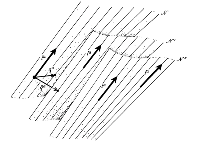
If a null congruence with tangent vector is hypersurface-orthogonal, then, by definition, the hypersurfaces to which it is orthogonal must be null, and is also tangent to them. Moreover, since the normal direction to a particular is unique at each point, and since is the only null direction orthogonal to , is the unique future-pointing null tangent direction at each point of . These directions in have a two-parameter family of integral curves called generators: they ‘form’ . Conversely, the generators of a one-parameter family of null hypersurfaces constitute a three-parameter family of null lines which are hypersurface-orthogonal. Note that the generators of the hypersurfaces , being null and hypersurface-orthogonal, must be geodetic by proposition 2.8.2. For the equivalence stated above the quantities and refer as well to the geometry of as to the entire congruence . We can speak of convergence and shear of a single null hypersurface. Therefore we have the following characterization.
Proposition 2.8.3.
A null congruence with tangent vector is hypersurface-orthogonal if and only if it is null-hypersurface forming, i.e. there exists a one parameter family of null hypersurfaces to which is tangent at each point.
2.9 Einstein’s Equations
The decomposition (2.6.15) of the Riemann tensor into its irreducible spinorial parts allows us to discuss the structure of space-time curvature, as is implied by Einstein’s Field Equations,
| (2.9.1) |
Here is the cosmological constant and the local stress-energy-momentum tensor.
Using (2.9.1) and (2.6.11)-(2.6.12) we get
from which, taking into account the trace-free property of ,
| (2.9.2) |
and thus
| (2.9.3) |
Thus, in terms of the spinors and and , introducing the spinor equivalent to the tensor and taking into account the first of (2.6.30), the field equations become
| (2.9.4a) | ||||
| (2.9.4b) | ||||
| (2.9.4c) | ||||
If we assume now that , i.e. in absence of matter, the previous equations reduce to
| (2.9.5a) | ||||
| (2.9.5b) | ||||
| (2.9.5c) | ||||
In particular equations (2.9.5a) is in a certain sense analogous to an actual field equation. It has a significance as being formally identical with the wave equation for a massless (zero rest-mass) spin 2-particle.
Chapter 3 Conformal Infinity
Abstract
In this part of the work the notion of conformal infinity, originally introduced by Penrose, is developed. The idea, which can be found in (Penrose, 1962), is that if the space-time is considered from the point of view of its conformal structure only, ‘points at infinity’ can be treated on the same basis as finite points. This can be done completing the space-time manifold to a highly symmetrical conformal manifold by the addition of a null cone at infinity, called . In this chapter we will first build up this kind of construction for Minkowski and Schwarzschild space-times and study their properties. Basing on these results we will give the definition of ‘asymptotic simplicity’. Owing to their conformal invariance, zero rest-mass fields can be studied on the whole of this conformal manifold, as will be done in the next chapter. It is worth noting that this method, which is deeply geometrical and coordinate-free, and hence more elegant, allows to obtain many results about the gravitational radiation in a very simple and natural way.
3.1 Introduction
The notion of ‘conformal infinity’ introduced by Penrose almost fifty years ago is one of the most fruitful concepts within Einstein’s theory of gravitation. Most of the modern developments in the theory are based on or at least influenced in one way or another by the conformal properties of Einstein’s equations in general or, in particular, by the structure of null infinity: the study of radiating solutions of the field equations and the question of fall-off conditions for them; the global structure of space times; the structure of singularities; conserved quantities; the null hypersurface formulation of General Relativity; the conformal field equations and their importance for the numerical evolution of space-times.
To introduce the notion of conformal infinity in a suitable way consider the situation of an isolated gravitating source. Then we might expect space-time to become ‘flat asymptotically’ as we move further away from it. How to formulate the concept of asymptotic flatness is a priori rather vague. Somehow we want to express the fact that the space-time ‘looks like’ Minkowski space-time at ‘large distances’ from the source. Obviously, the investigation of asymptotic properties depends critically on how we approach infinity. In order to fix ideas, consider an isolated gravitational system that emits gravitational waves carrying positive energy, as consequence of its varying asymmetry (Stewart, 1991; Penrose, 1967). To find out what energy we should assign to the waves, it is necessary to measure the masses and respectively before and after the emission and then evaluate the difference . One way to measure the mass would be to integrate some expression of mass density over a spacelike hypersurface ; however in this case we should take into account the non-local mass density of the gravitational field itself. To avoid those complicated effects a good idea would be to take the hypersurface , which can be chosen to be a 2-surface, to infinity, where the curvature should become in some way‘small ’ for an asymptotically flat space-time. The mass measure obtained in this way is called ADM mass. But if we were taking in the same way a spacelike 2-surface that intercepts the source after the emission of gravitational radiation, we wouldn’t get as our mass measurement, but again . This is because such a would intercept, in addiction to the source worldline, the radiation ones too, giving a total mass measure .
To obtain a correct measurement of we should bend so that the already emitted radiation remains in its past, never intersecting it. As a consequence we pick to be a null surface at far distances from the source and the corresponding mass we obtain is called Bondi mass. The measurement of can be done by using a null 2-surface too. We denote the two null surfaces used by e .


The main question now is to understand how to take the above limits to infinity in an appropriate way and to express properly the concept of asymptotic behaviour. While it is certainly possible to discuss asymptotic properties by taking carefully limits as ‘’, there is an equivalent way to approach the problem, introduced by Penrose, which allows us to avoid such limit operations and that possesses a more geometrical nature, based on the concept of space-time conformal rescalings. As we will see the main feature of those transformations will be to ‘make infinity finite’ in a certain way.
3.2 Conformal Structure of Minkowski and
Schwarzschild Space-Times
The idea (Penrose, 1962; Penrose, 1963; Penrose, 1964; Penrose, 1967) is to construct, starting from the ‘physical space-time’ , another ‘unphysical space-time’ with boundary (see Appendix A), such that is conformally equivalent to the interior of with , given an appropriate function . The two metric and define on the same null-cone structure. The function has to vanish on , so that the physical metric would have to be infinite on it and cannot be extended. The boundary can be thought as being at infinity, in the sense that any affine parameter in the metric on a null geodesic in attains unboudedly large values near . This is because if we consider an affinely parametrized null geodesic in the unphysical space-time with affine parameter , whose equation is
it is easy to see that the corresponding geodesic in the physical space-time with affine parameter is solution of the equation
where a ′ denotes a derivative. If we want the parameter to be affine the right hand side of the above equation must vanish, and hence we must have
where is an arbitrary constant. Since on , diverges and hence never reaches , which apparently really is at infinity. Thus, from the point of view of the physical metric, the new points (i.e. those on ) are infinitely distant from their neighbours and hence, physically, they represent ‘points at infinity’.
The advantage in studying the space-time instead of is that the infinity of the latter gets represented by a finite hypersurface and the asymptotic properties of the fields defined on it can be investigated by studying and the behaviour of such fields on .
However, there is a large freedom for the choice of the function . Anyway, it will turn out from general considerations that an appropriate behaviour for is that it should approach zero (both in the past and in the future) like the reciprocal of an affine parameter on a null geodesic of the space-time considered ( as ).

Consider physical Minkowski space-time in spherical polar coordinates
| (3.2.1) |
where
| (3.2.2) |
Introduce now the standard retarded and advanced null coordinates defined by
The coordinates and serve as affine parameters into the past and into the future of null geodesics of Minkowski space-time.
The metric tensor becomes
Consider now the unphysical metric
with the choice
Note that for we have , , as pointed out before.
Now to interpret this metric it is convenient to introduce new coordinates
such that we have
| (3.2.3) |
It is possible to bring the metric (3.2.3) in a more familiar form by setting
from which follows
| (3.2.4) |
It’s worth noting that the metric (3.2.4) is that of Einstein static universe, , the cylinder obtained as product between the real line and the 3-sphere, . However the manifold represents just a finite portion of such cylinder.

The metric (3.2.3) is defined at and : those values correspond to the infinity of and therefore they represent the hypersurface . Hence we have defined a conformal structure on , whose coordinates are free to move in the range . The boundary is given by or and the interior of is conformally equivalent to Minkowski space-time.
We introduce the following points in :
- •
, called future timelike infinity given by the limits , , , , . All the images in of timelike geodesics terminate at this point;
- •
, called past timelike infinity given by the limits , , , , . All the images in of timelike geodesics originate at this point;
- •
, called spacelike infinity given by the limits , , , , , , . All spacelike geodesics originate and terminate at this point.
We also introduce the following hypersurfaces in :
- •
, called future null infinity, is the null hypersurface where all the outgoing null geodesics terminate and is obtained in the following way. Null outgoing geodesics are described by , with finite constant, from which and . Taking the limit we get and , hence and with . In coordinates and . As runs in its range of values this is a point moving on the segment connecting e . All outgoing null geodesics terminate on this segment, described by the equation .
- •
, called past null infinity, is the hypersurface form which all null ingoing geodesics originate. It can be shown that this is given by the region and and is described, in terms of coordinates, by the segment of equation connecting and .
Putting
the two equations defining the hypersurfaces and are
respectively. The normal covectors to and are
Since it follows that and are null hypersurfaces.
At this stage, we can build some useful representation of the space-time . One is a portion of the plane in coordinates, that is an example of Penrose diagram. Each point of the Penrose diagram represents a sphere , and radial null geodesics are represented by straight lines at , see Figure 3.4

Another one is depicting as a portion of the cylinder , see Figure 3.3.
One more representation for the Minkowski space-time is furnished by Figure 3.5.

We note here that for the points , and are regular and that and both have topology. Furthermore the boundary of is given by .
Consider now Schwarzschild space-time, defined by the metric
| (3.2.5) |
Introducing coordinates as
| (3.2.6) |
we have
| (3.2.7) |
The first of (3.2.6) is just the null retarded coordinate, corresponding to a null outgoing geodesic. Note that the coordinate in (3.2.6) is the usual Wheeler-Regge ‘tortoise coordinate’ introduced in Wheeler and Regge (1957). Consider now the unphysical metric
| (3.2.8) |
Schwarzschild space-time, , is given by because . We remark that the Schwarzschild solution can easily be extended beyond the event horizon, i.e. and because the apparent singular point of the metric (3.2.5) is just a coordinate singularity and not a physical one, how can be noticed from (3.2.7). The metric (3.2.8) is defined for (i.e. ) and hence for we may take the range , such that the hypersurface is given by .
Re-expressing (3.2.8) in terms of a null advanced coordinate
corresponding to a null ingoing geodesic we get
| (3.2.9) |
By doing this it is now possible to introduce as the hypersurface of described by (3.2.9) for .

It is easy to check that the hypersurfaces and , given by the equations are again null hypersurfaces.
The main difference between the Minkowski space-time case emerges from the fact that the points , and in the Schwarzschild case are not regular, as could be deduced by the study of the eigenvalues of the Weyl tensor. However it should not be surprising that and turn out to be singular, since the source generating the gravitational field becomes concentrated at these points, at the two ends of its history. Thus we will omit , and from the definition of , that will just be . We have two disjoint boundary null hypersurfaces and each of which is a cylinder with topology . These null hypersurfaces are generated by rays (given by ,constant, ) whose tangents are normals to the hypersurfaces. These rays may be taken to be the of the topological product .
Take now into account a space-time with metric tensor (Penrose and Rindler, 1986; Penrose, 1967)
| (3.2.10) |
with , and sufficiently differentiable functions (say ) of , with , on the hypersurface defined by and in its neighbourhood. If the determinant
does not vanish, the space-time with metric , being ,
is regular on . It is clear that Schwarzschild space-time is just a particular case of this more general situation described by (3.2.10). Furthermore this metric includes all the Bondi-Sachs type (with which we will deal in chapter 6). These metrics describe a situation where there is an isolated source (with asymptotic flatness) and outgoing gravitational radiation. Hence a regularity assumption for seems a not unreasonable one to impose if we wish to study asymptotically flat space-times and allow the possibility of gravitational radiation. In such situations, therefore, we expect a future-null conformal infinity to exist. The choice made for possesses the important property that its gradient at , , is not vanishing and hence defines a normal direction to ( being described by the equation ).
Roughly speaking, to say that a space-time is asymptotically flat means that its infinity is ‘similar’ in some way to the Minkowski’s one. As a consequence we may expect the conformal structure at infinity of an asymptotically flat space-time to be similar to the one found for the Minkowski case.
With those ideas in mind we may now proceed to a rigorous definition of asymptotically simple space-time. However we must also bear in mind that asymptotically flatness is, in itself, a mathematical idealization, and so mathematical convenience and elegance constitute, in themselves, an important criteria for selecting the appropriate idealization.
3.3 Aymptotic Simplicity and Weak Asymptotic Simplicity
Definition 3.3.1.
A space-time is -asymptotically simple if some smooth manifold-with-boundary exists, with metric and smooth boundary such that:
- 1.
is an open submanifold of ;
- 2.
there exists a real valued and positive function , that is throughout , such that on ;
- 3.
and on ;
- 4.
every null geodesic on has two endpoints on .
The space-time is called physical space-time, while unphysical space-time.
Definition 3.3.2.
Hawking and Ellis (1973) A space-time is -asymptotically empty and simple if it is -asymptotically simple and if satisfies the additional condition
- 5.
on an open neighbourhood of in (this condition can be modified to allow the existence of electromagnetic radiation near ).
Remark 3.3.1.
Note that there are many different definitions of asymptotic simplicity. We used here the one which is due to Penrose and Rindler (1986), but others which slightly differ from this are possible (Penrose, 1967; Hawking and Ellis, 1973; Stewart, 1991).
Remark 3.3.2.
Note that although the extended manifold and its metric are called ‘unphysical’, there is nothing unphysical in this construction. The boundary of in is uniquely determined by the conformal structure of and, therefore, it is just as physical as .
Now we try to justify the previous assumptions.
Clearly with , and we mean to build as the null infinity of , using the results obtained in the Minkowski case, with which must share some properties. Condition ensures that the whole of null infinity is included in . Furthermore null geodesics in correspond to null geodesics in because conformal transformations map null vectors to null vectors: the concept of null geodesic is conformally invariant. Thus we deduce that past and future infinity of any null geodesic in
are points of . Condition ensures that the physical Ricci curvature vanishes in the asymptotic region far away from the source of the gravitational field. Finally note how the points , and are excluded from the definition of , since is not a smooth manifold at these points. The condition , together with , implies that for an asymptotically empty and simple space-time the conformal infinity is always null. This is because it is easy to see that the Ricci scalar of the metric is related to the Ricci scalar of the metric by
and hence, by multiplying both members by , and by evaluating this equation on where , it follows that . By condition , since , it follows that and thus , the normal vector to is null and, by definition, is a null hypersurface. Furthermore is related to by
Since is null and is defined on , if condition holds, the previous equation on leads to
Contracting with it gives
Hence the normal vector to is divergence- and shear-free. Furthermore it will be pointed out in chapter 4 that for any asymptotically simple space-time consists of two disconnected components, on which null geodesics in have their future endpoints and on which they have their past endpoints and both and have the topology , so that the structure of the conformal infinity found for Minkowski space-time is that of any asymptotically simple space-time. The following theorem is very important because it states the relation that occurs between an asymptotically simple space-time and its causal structure.
Theorem 3.3.1.
An asymptotically simple and empty space-time is globally hyperbolic.
The proof can be found in Hawking and Ellis (1973). The interpretation of this result is the following. If a space-time has a certain structure at infinity that resembles the one of Minkowski, then it is ‘predictive’ in the sense specified in section 1.7 and is causally stable and thus there cannot occur any causality violations.
The asymptotic simplicity is a very strong assumption for a space-time.
However condition is difficult to verify in practice and is not even satisfied by some space-times that we would like to classify as asymptotically flat. As an example, for Schwarzschild space-time, it is known that there exist null circular orbits with radius , and hence don’t terminate on . For this reasons condition is often too strong and gets replaced by a weaker one that brings to the notion of weakly asymptotically simple space-time.
Definition 3.3.3.
A space-time ( is weakly asymptotically simple if there exists an asymptotically simple space-time with associate unphysical space-time , such that for a neighbourhood of in , the region is isometric to a similar neighbourhood of .
In this way a weakly asymptotically simple space-time possesses the same properties of the conformal infinity of an asymptotically simple one, but the null geodesics do not necessary reach it because it may have other infinities as well. Such space-times are essentially required to be isometric to an asymptotically simple space-time in a neighbourhood of . A different condition has been proposed by Geroch and Horowitz (1978) In the remainder for asymptotically flat space-time we will mean a weakly asymptotically simple one.
Chapter 4 Conformal Rescalings and
Abstract
In this chapter we will make a direct application of the spinor formalism to the conformal technique, both concepts being introduced in the previous parts of the work. We will study the behaviour of the spinor fields under conformal rescalings and, in particular, that of zero rest-mass fields. This is motivated by the fact that the equation of motion of the Weyl spinor, as shown in section 2.9, is that of a spin 2 zero-rest mass field. Generally, if we find a way to solve an equation on the unphysical space-time and the fields involved behave in a suitable way under conformal rescalings, then we are able to reconstruct the solution on the physical space-time too. In the last section we show the basic properties of for an asymptotically flat space-time. These are (under the assumption that the vacuum Einstein’s equations hold and hence the cosmological constant equals zero):
- •
is a null hypersurface;
- •
has two connected components, and , each of which has topology ;
- •
the conformal Weyl tensor vanishes on ;
- •
is shear-free.
4.1 Conformal Rescalings Formulae
Before exploring asymptotic properties we need to establish the relationship between the connection and curvature tensors in the physical and unphysical space-times. As we have seen in chapters 2 and 3 a conformal rescaling is a transformation that maps the physical metric to the unphysical one via
| (4.1.1) |
being a smooth and positive real valued function that vanishes on . Note that no transformation of points is involved. Thus we can set, consistently with the transformation of the metric and with (2.3.3),
| (4.1.2) |
The only alternative to this choice, , is not continuous with the identity scaling and is therefore rejected. We note here that we could have chosen a complex in (4.1.2) and hence replaced with in (4.1.1), but this would naturally give rise to a torsion, as discussed in Penrose (1983). By choosing a real we get for the conjugates
We establish now the following convention: if the kernel letter of a spinor carries a tilde then , are to be used; however if there is no such tilde then the standard , are used.
As we mentioned above, a spin vector has a definite geometric interpretation (flag and flagpole) which is quite independent of any rescaling. Hence we can suppose a conformal rescaling (4.1.2) to leave unaffected
Then for the associate spin co-vector we have
Thus is a conformal density of weight 1, i.e. a quantity that gets multiplied by under a rescaling.
More generally, it is convenient to work with conformal densities of arbitrary weight.
Definition 4.1.1.
Define to be a conformal density of weight k if it is to change under a rescaling (4.1.2) to
Normally is integer or half-integer. Observe that , , , have respective conformal weights 2,1,-1,-2. Consequently, whenever a spinor (tensor) index is raised its conformal weight is reduced by unity (2), and whenever a spinor (tensor) index is lowered its weight is increased by unity (2).
We also require now a spinor covariant derivative for the unphysical space-time, . To find the right expression for such a covariant derivative we need to note that under the conformal rescaling (4.1.1) the Christoffel symbols
transform as
Some experimentation shows that the only plausible candidate is defined via the rules
- 1.
for all scalars ;
- 2.
- 3.
- 4.
;
where . The formal existence and uniqueness proof is given in Penrose and Rindler (1984). We know from the property of that
Hence, taking into account the definition of and (2.2.3) we get
Thus, having defined the above transformation properties of the covariant derivative, it naturally follows that if the compatibility condition holds for then it holds for too.
The transformation formulae for the various parts of the Riemann tensor are quite complicated and deriving them from (2.6.26) and (2.6.27) is a tedious, but simple exercise. They are
| (4.1.3) | ||||
| (4.1.4) | ||||
| (4.1.5) |
In vector form the last two equations are
| (4.1.6) | ||||
| (4.1.7) |
where .
We see from (4.1.3) that is conformally invariant as claimed before. It is a measure of the part of the curvature that remains invariant under conformal rescalings. Since in flat space-time, it vanishes also in conformally flat space-time.
Note that due to equation (2.6.16) we have under conformal rescalings the following behaviours for the Weyl tensor
| (4.1.8) |
4.2 Zero Rest-Mass Fields
As mentioned above, the first of equations (2.9.5) describes the dynamic of a massless free field of spin 2. It is useful to discuss zero rest-mass fields of arbitrary (half or half-integer) spin and their radiation properties in general. In fact they exhibit a certain characteristic asymptotic behaviour, that has been called by Sachs the peeling-off property (Sachs, 1961; Sachs, 1962b).
A field of spin , where is a positive integer, is generally described by a spinor with indices. Let be totally symmetric in its indices:
| (4.2.1) |
The massless free-field equation for spin is then taken to be
| (4.2.2) |
The Bianchi identity has this form in empty space, with taking the place of . It is thus a curved-space spin-2 field equation. Similarly, the source free Maxwell equations have this form with (spin 1) taking the place of (equation (2.7.4)). The Dirac-Weyl equation for the neutrino also falls into this category, with (spin 1/2).
To establish the conformal invariance of (4.2.2), it is convenient first to re-express that equation in a different form.
We have
thus (4.2.2) is, taking into account the symmetry property (4.2.1), equivalent to
| (4.2.3) |
Now choose to be a conformal density of weight -1.
| (4.2.4) |
Then we have, using the property of the covariant derivative of the unphysical space-time,
| (4.2.5) |
Now the RHS of (4.2.5) beyond the first term is automatically symmetric in . Consequently the LHS is symmetric in if and only if (4.2.3) holds. But that means that (4.2.3) is conformally invariant, i.e.
We can thus give the following:
Proposition 4.2.1.
If a totally symmetric spinor is a conformal density of weight -1 then equation (4.2.2) is conformally invariant.
Hence for a spin-2 massless field we should have
| (4.2.6) |
However from equation (4.1.3) we see that is a conformal density of weight 0, i.e. conformally invariant. Thus equation (2.9.5)
| (4.2.7) |
is not invariant under rescalings. This is related to the fact that the equations of General Relativity are not conformally invariant. Suppose we have a solution of (4.2.7). Putting and transforming according to (4.2.6) we have
| (4.2.8) |
from which
i.e.
A conformal rescaling applied to a solution of Einstein’s equations will, therefore, generally destroy the satisfaction of the vacuum equations.
Furthermore in curved space-times there is an algebraic consistency condition for equation (4.2.2) that holds for , called the Buchdahl constraint (Buchdahl, 1958). To obtain this relations apply to (4.2.2)
where the symmetry of in and definition (2.6.23) have been used. Now using the generalization to many index spinors of first of (2.6.26) we get
Each of the first two terms of the LHS involves, because of the symmetry of , the term that vanishes because of (2.6.4). The other terms of LHS involve , this equation coming from the definition (2.6.14). Hence we have, for ,
| (4.2.9) |
Thus, if , equation (4.2.9) implies an interconnection between and the conformal curvature spinor .
4.3 Properties of
Assume now that Einstein Field Equations
| (4.3.1) |
hold in an weakly asymptotically simple space-time with conformal infinity , given by the equation
Hence, putting
| (4.3.2) |
by the property of the definition of asymptotic simplicity it follows that on and, being orthogonal to each locus , it constitutes a normal to at each of its points.
For the time being, we shall allow some massless matter fields in the neighbourhood of , so that . From equations (2.9.2) and (2.6.12) we get
| (4.3.3) |
near (where ‘near ’ means in , for some neighbourhood of in the unphysical space-time ). Now define the quantity
Using equation (2.6.11) and (2.6.12) we get
From (4.3.3) if we evaluate the trace we get
| (4.3.4) |
But from the transformation properties (4.1.6) and (4.1.7)
then evaluating the trace again gives
| (4.3.5) |
Comparing (4.3.4) and (4.3.5) we obtain on (set )
and thus
| (4.3.6) |
Equation (4.3.6) yields the following:
Proposition 4.3.1.
If the trace of the energy tensor vanishes near , then is spacelike, timelike, or null according as is positive, negative, or zero.
When is null, it consists naturally of two disconnected pieces, and , since lies locally to the past or future of it. A point of lies on () if the interior of its past (future) light cone lies in .
There is an important theorem which regards the structure of when it is null.
Theorem 4.3.1.
In any asymptotically simple space-time for which is everywhere null, the topology of each of is given by
| (4.3.7) |
and the rays generating can be taken to be the factors.
We give here a sketch of the proof.
Proof.
If the space-time is asymptotically simple, it is globally hyperbolic (3.3.1) and thus it has a Cauchy surface . Let denote the collection of all null geodesic in and be a point of . The set of null geodesics emanating from is just the set of null directions at and hence is, topologically, a 2-sphere . Therefore the topology of is since, by theorem 1.7.9, all null geodesics intersect . Let be a point of . The set of null geodesics emanating from is a 2-sphere. However, one of these null geodesics lies in , and so does not enter . Hence, the null geodesics from which do not enter are, topologically, a 2-sphere minus a single point, i.e. a plane . Hence is topologically since all null geodesics intersect . But is the union of its null generators, and so we have , where is some 2-manifold. It follows that and thus . It can be shown that the last equation can hold only if is topologically a 2-sphere and is topologically (see Geroch, 1971, pg. 99). We have obtained . ∎
Remark 4.3.1.
The first proof of this theorem, involving sophisticated arguments, is due to Penrose (1965). However, as remarked in Newman (1989), the arguments carried out by Penrose were incorrect, and a more rigorous proof can be found in Geroch (1971) or in Hawking and Ellis (1973).
Remark 4.3.2.
Since , as shown, is topologically , is topologically . That is, every asymptotically simple space-time is topologically the same as Minkowski space.
Thus , when it is null, it fairly resembles the infinity of Minkowski space-time, each of containing null generators. The occurrence of this situation distinguishes an asymptotically simple space-time in which is null from one in which is spacelike.
In order to proceed further and to obtain more results concerning the structure of we shall impose that Einstein vacuum equations hold near . It can be shown that in other certain cases when does not vanish near , i.e. the vacuum equations are not appropriate to describe the space-time, the consequences are almost the same, but the derivation is more involved (Penrose, 1965). An example of this is the case in which Einstein-Maxwell equations hold near . Hence we restrict ourselves to the Einstein vacuum equations, assuming that when matter is present the results still hold for .
From equation (4.1.7) and the second of (2.9.5) we have
Multiplying by both sides of previous equation, assuming for and hence that must be continuous at , we obtain on the asymptotic Einstein condition
| (4.3.8) |
where we introduced the ‘weak equality’ symbol . Considering two spinor fields and , saying that
| (4.3.9) |
means that on . We have to be careful when taking the derivatives of a weak equation, bearing in mind that only tangential derivatives can be relied upon to obtain a new weak equation. Hence from (6.4.10) we could get correctly
but not . In the remainder we could drop the phrase ‘near ’, replacing the equality symbol with the weak equality one. Obviously we have
Equation (4.3.6) can be written in the form
| (4.3.10) |
and (4.3.8) as
| (4.3.11) |
In the case of null we can put
| (4.3.12) |
introducing a N-P tetrad of vectors as done in (2.3.2) and with a non-zero scalar. Multiplying the first of (4.3.11) by we get
| (4.3.13) |
i.e. the null congruence with tangent vector is shear-free. Also, from (4.3.2), this congruence is rotation free, i.e. (this last condition is trivial and follows from the fact that is null).
We can finally say that when is a null hypersurface it is generated by the two-parameter family of integral curves of , whose null congruence is shear- and rotation-free. The fact that and have this kind of structure is essential for the definition of the BMS group, which will be done later, in chapter 6.
Theorem 4.3.2.
If the vacuum equations hold near , then the Weyl tensor
Proof:
From the Bianchi identity in spinor form (i.e. equation (2.9.5)) we have for the physical space-time
. By (4.2.8) and (4.1.3) we obtain
in , that implies
| (4.3.14) |
which, by continuity, holds on . Hence
| (4.3.15) |
From (4.3.10) we have . Thus, if , the matrix is non-singular and can be inverted so that we have
from which the result follows.
The case in which is more difficult. The sketch of the proof we are giving here depends upon a global result requiring the topology (4.3.7). From equations (4.3.15) and (4.3.12) we have
i.e., by 2.5.2
| (4.3.16) |
for some . Applying to (4.3.14) we get
Lowering and symmetrizing over it becomes
Using the complex conjugate of equation (4.3.11) the last term vanishes and we obtain
hence, raising
By theorem 2.2.1 we obtain
thus
From symmetry properties of spinors (Penrose and Rindler, 1984) it can be shown that the previous equation implies
Again it can be shown (Penrose and Rindler, 1984) that this equation on any spherical cross-section of admits the solution on the sphere, whence the proof is complete. ∎
We refer to the conditions
| (4.3.17) |
as the strong asymptotic Einstein condition.
It is now important to mention the following general result.
Lemma 4.3.1.
Let be a weakly asymptotically simple space-time and let be a neighbourhood of in . Suppose to be a (with ) spinor that satisfies . Then there exists a spinor such that .
An outline of the proof can be found in Penrose and Rindler (1986), pg. 357.
In section 4.2 we noted the difference in the conformal behaviour of the Weyl spinor with that of a massless spin-2 field . We define now a specific massless spin-2 field
that, under a rescaling (4.1.2), transforms as
| (4.3.18) |
In that way the zero rest-mass field equation for is conformally invariant. We thus have
| (4.3.19) |
As it stands is not defined on . But theorem 4.3.2, lemma 4.3.1 and the assumption of smoothness allow the extension of to the boundary as a smooth field on . Note that applying to (4.3.18) we obtain
| (4.3.20) |
and thus, on we obtain from the derivative of the Weyl spinor.
will be called the gravitational field. From the above discussion is a genuine spin-2 field with the natural conformal behaviour and can be thought to describe the gravitational effects. In particular its values on the boundary are closely related to the gravitational radiation which escapes from the system under consideration and hence the behaviour of its components at is fundamental in the understanding of gravitational radiation theory, which can be analysed with the Sachs peeling property that we are going to investigate for a general spin field with a generic conformal weight. The basic idea, which will be developed in the next chapter is the following: consider a space-time which allows us to attach a conformal boundary, thus defining an unphysical space-time conformally related to the given space-time. Suppose we are also given a solution of a conformally invariant equation on this unphysical manifold, as the first of (4.3.19). Then there exists a rescaling of that unphysical field with power of the conformal factor, which produces a solution of the equation on the physical manifold. Now suppose that the unphysical field is smooth on the boundary. Then the physical solution will have a characteristic asymptotic behaviour which is entirely governed by the conformal weight of the field, i.e. by the power of the conformal factor used for the rescaling. Thus, the regularity requirement of the unphysical field translates into a characteristic asymptotic fall-off or growth behaviour of the physical field, depending on its conformal weight. Penrose used this idea to show that solutions of the zero rest-mass equations for arbitrary spin on a space-time, which can be compactified by a conformal rescaling, exhibit the peeling property in close analogy to the gravitational case as discovered by Sachs. Take as an example the spin-2 zero rest-mass conformally invariant equation (4.3.19) for the field which is a conformal density of weight 1. Then, assuming a regularity condition of the unphysical field , we would have that falls asymptotically as does.
Chapter 5 Peeling Properties
Abstract
In this part of the work we carry out a detailed proof of the so-called peeling property. This will be done using the spinor formalism only. Hence, many of the notions introduced in chapter 2 will be useful here. The peeling property is a characteristic fall-off behaviour of the fields at infinity, in asymptotically flat space-times. Of particular importance for our purposes is the application of the peeling property to zero rest-mass fields. In fact it allows us to find the behaviour of the Weyl spinor that, as already remarked, can be used to build a spin 2 massless gravitational field. We will show that this behaviour is described by a sum of negative powers of , where is the affine parameter along null geodesics.
5.1 Introduction
The peeling, or peeling-off of principal null directions is a generic asymptotic behaviour which was firstly developed for spin 1 and spin 2 fields in the flat case by Sachs (1961) and in the asymptotically flat case by Sachs (1962b). In his works Sachs proposed an invariant condition for outgoing gravitational waves. The intuitive idea was that at large distances from the source, the gravitational field, i.e. the Riemann tensor of outgoing radiation, should have approximately the same algebraic structure as does the Riemann tensor for a plane wave. As one approaches the source, deviations from the plane wave should appear. Sachs analysed these deviations in detail, using the geometry of congruences of null curves, and obtained rather pleasing qualitative insights into the behaviour of the curvature in the asymptotic regime. The notion was explored further in Newman and Penrose (1962), in which the authors formulated what has become known as the Newman-Penrose formalism (that we developed in section 2.7) that combined the spinor methods, which had been developed earlier in Penrose (1960), with the (null-)tetrad calculus already used. In particular they applied their formalism to the problem of gravitational radiation using a coordinate system which was very similar to the one used by Sachs (1961) and showed that the single assumption already implied the peeling property as stated by Sachs. In the next years Penrose, guided by the idea of ‘following the field along null directions’, formulated the concept of the conformal structure of the space-time, and in Penrose (1965) the conformal method is used, together with the spinor formalism, to deduce the peeling properties. In this work the basic qualitative picture we have today is developed. In the remainder of this chapter we will use Penrose approach (that was further improved in Penrose and Rindler (1986)) to derive the peeling property. The proof of the peeling properties depends strongly on the comparison between two parallelly propagated spin frames along a null geodesic with respect to the two metrics and .
5.2 Parallelly Propagated Spin-Frames
Let be a null geodesic in reaching at the point . We choose a spin frame at one point of , where the tangent vector is , and propagate the basis parallelly along , as in section 2.8, via
| (5.2.1) |
where . Ler be an affine parameter on :
We can choose whatever conformal transformation for behaviour for and provided that transforms according to (4.1.2). If we take
| (5.2.2) |
then the propagation equation (5.2.1) is preserved. In fact we have, using rule of section 4.1 and equations (5.2.1) and (5.2.2)
We can complete to a spin frame and arrange
| (5.2.3) |
where we set, to preserve (4.1.2),
| (5.2.4) |
with scalar function to be determined. Using the second of (5.2.3) we get
hence
| (5.2.5) |
where
| (5.2.6) |
We compare now affine parameters on . We take to be an affine parameter on , with origin at and with tangent vector . We have
The symbol now means equality at . We have of course and by condition of definition 3.3.1 on . Thus we can set
| (5.2.7) |
Note that
| (5.2.8) |
so this coincides with the one of (4.3.12). Using the smoothness of it follows that
| (5.2.9) |
, , …being constant.
From the asymptotic Einstein condition (4.3.8) we have, using equation (2.8.3) ( is an affine parameter for ):
Thus in expansione (5.2.9) we have . Consider
hence
| (5.2.10) |
all and coefficients being constant on and being the constant of integration. For large values of we can invert (5.2.10) to obtain
| (5.2.11) |
which, substituted back into (5.2.9), yelds the following expansion for :
| (5.2.12) |
the and coefficients being again constant on .
The form we just found for justifies the assumption made in section 2.2, according to which the conformal factor should behave like the reciprocal of an affine parameter along any null geodesic. In fact here we have, by (5.2.12), as .
5.3 Comparison Between the Spin-Frames
We proceed now to the comparison between the spin frames. By (5.2.4) we see that
| (5.3.1) |
We would like to choose the function such that at the point , so that the two spin frames coincide at that point, i.e. and . Integrating equation (5.2.5) would give
that, using expansion (5.2.9), yields the behaviour
Hence we are forced to require to ensure that the two spin frames coincide at . By equation (5.2.6) this condition means that must be, at , a linear combination of and of , so that its transvection with vanishes. We thus write
| (5.3.2) |
We have so that of (5.3.2) is the same of (5.2.8). The second term has been chosen to have that form because it satisfies , just as in equation (4.3.10).
With this choice for , equation is satisfied. Hence it is reasonable to assume , using lemma 4.3.1. With this assumption integration of (5.2.5) yields, using (5.2.7)
This would give, as required, , but actually it turns out that vanishes to second order at , i.e. , so the logarithm is eliminated. This elimination is very important becauase the presence of a logarithm would destroy the power series we are looking for.
Consider in fact the difference between the two members of (5.3.2). It has to vanish at . Hence, by 4.3.1, there exists a ( is being the derivative of , that is ) covector , defined along , such that
| (5.3.3) |
Acting on this with , we get
and, after transvecting with ,
The last two terms vanish by (5.2.3). Using equation (5.2.8) we get and using the Einstein asymptotic condition (4.3.11) , hence on
Then by lemma 4.3.1 there exists some function on such that
| (5.3.4) |
Using equation (5.3.4) and (5.3.3) then we get that (5.2.6) becomes
Hence
that is regular in . Thus we can write the expansion
being the constant of integration, that becomes, using (5.2.11)
Thus, using (5.2.12)
Eventually equation (5.3.1) and the second of (5.2.2) become
| (5.3.5) |
that are the relations between the spin frames we were looking for.
5.4 Proof of the Peeling Property
Consider now a conformal density of weight
| (5.4.1) |
and suppose to be with at . Under this hypothesis the following expansion holds
| (5.4.2) |
Consider a typical component
with a total number of zero indices ( and ) and the corresponding component with respect to the frame ,
The expansion (5.4.2) applies to every component, hence:
which, in terms of (using equation 5.2.11) becomes, renaming the constants of the expansion
| (5.4.3) |
We have, transvecting (5.4.1) with the basis vector and ,
As next we insert relations (5.3.5) in the previous equation:
which, for large ’s becomes
Using the expansions (5.2.12) and (5.4.3) we get
Again, for large values of we can neglect the terms beyond the first in the first sum and thus obtain, renaming the parameters of the expansion (which remain constant along )
We can eventually state the peeling property for the field :
| (5.4.4) |
where is constant along . We note that the leading term in the expansion (5.4.4) is a multiple of .
5.5 Applications to Massless Fields
Consider a massless field of arbitrary spin , described by a totally symmetric spinor field with indices, of weight , so that the massless field equation is conformally invariant. Suppose that is at . Then if we consider the various components , ,…, their behaviour is the following:
| . | |||
| . | |||
| . | |||
where are constant on .
Consider now electromagnetism. In section 2.7 we have seen that, starting from , we could build three scalars, , and . Using (5.4.4) we get that each of this scalars has the following expansion in decreasing powers of :
Furthermore, using (2.7.3) we can write
| (5.5.1) |
which schematically is
The leading term proportional to is the radiation part of the electromagnetic field. It is of type N or null, according to the Petrov classification, and is the component of totally contracted with .
In the case of gravity we have, following the same procedure of (2.7.3),
| (5.5.2) |
Due to the peeling property (5.4.4) we have the following expansions:
Hence we can express (5.5.2) as
| (5.5.3) |
which can be written schematically as
| (5.5.4) |

In particular, , which may be thought of as describing the gravitational radiation field, can be identified with that component of on which is totally contracted with . Note that the part of the curvature which has no relation to the null direction of the outgoing geodesic goes as , and hence to that order the curvature is not related to the geodesic.
This argument can be carried out more generally. In fact, we can always decompose a spin massless field as
where
This is the generalization of equations (5.5.1) and (5.5.3) to an arbitrary spin field.
Consider now the transvection of with ’s:
| (5.5.5) |
This transvection always vanishes because in there are at least ’s and hence in (5.5.5) there must be at least one term of the form . From equation (5.5.5) and proposition 2.5.1 we see that , and hence the term of that behaves like , has always at least principal null directions pointing along the direction of , i.e. along . In particular the part, what we call the radiation field, is always null.
Chapter 6 Bondi-Metzner-Sachs Group
Abstract
Minkowski space-time has an interesting and useful group of isometries. But for a general space-time, the isometry group is simply the identity and hence provides no significant informations. Yet symmetry groups have important role to play in physics; in particular, the Poincaré group, describing the isometries of Minkowski space-time plays a role in the standard definitions of energy-momentum and angular-momentum. For this reason alone it would seem to be important to look for a generalization of the concept of isometry group that can apply in a useful way to suitable curved space-times. The curved space-times that will be taken into account are the ones that suitably approach, at infinity, Minkowski space-time. In particular we will focus on asymptotically flat space-times. In this chapter the concept of asymptotic symmetry group of those space-times will be studied. In the first two sections we derive the asymptotic group, which is referref to as ‘BMS’, by Bondi, Metzner and Sachs, following the classical approach which is basically due to Bondi et al. (1962); Sachs (1962b); Sachs (1962a). This is essentially the group of transformations between coordinate systems of a certain type in asymptotically flat space-times. In the third section the derivation is made following arguments developed by Penrose, which involve the conformal structure (which we carried out in chapter 3), and is thus more geometrical and fundamental (Newman and Penrose, 1966; Penrose, 1972a; Penrose and Rindler, 1986; Stewart, 1991). In the remaining sections we will discuss the properties of the BMS group, such as its group structure, its algebra and the possibility to obtain as its subgroup the Poincaré group, as we may expect.
6.1 Introduction
The importance of the concept of energy within a physical theory, if introduced correctly, arises from
the fact that it is a conserved quantity in time and hence a very useful tool.
Thus, in general relativity one of the most interesting questions is related to the meaning of gravitational energy.
Starting from any vector that satisfies a local conservation equation, that can be put in the form
| (6.1.1) |
one can deduce an integral conservation law which states that the integral over the boundary of some compact region of the flux of the vector across this boundary necessarily vanishes. In fact, using Gauss’ theorem we have
| (6.1.2) |
Now we know that in General Relativity the energy-momentum tensor satisfies the local conservation law
| (6.1.3) |
which follows directly from the Einstein field equations. However from (6.1.3) we cannot deduce any conservation law. This is because in this case the geometric object to integrate over a 4-volume (as on the right-hand side of (6.1.2)) would be a vector and we can not take the sum of two vectors at different points of a manifold. This picture is ameliorated if space-time possesses symmetries, i.e. Killing vectors. If is a Killing vector,
we may build the vector
that satisfies (6.1.1), since
The second term vanishes because is symmetric and so . Therefore the presence of Killing vectors for the metric leads to an integral conservation law. In flat Minkowski space-time we know that there are 10 Killing vectors:
where is +1 if and -1 if . The first four generate space-time translations
and the second six ‘rotations’ in space-time (these are just the usual ten generators of
the inhomogeneous Lorentz group). One may use them to define ten vectors and
which will obey (6.1.1). We can think of as representing the flow of
energy, and , and as the flow of the three components of linear
momentum. The can be interpreted as the flow of angular momentum. If the metric is
not flat there will not, in general, be any Killing vectors. It is worth noting that the diffeomorphism group
has, for historical reasons, frequently been invoked as a possible substitute for the Poincaré group for a
general space-time. However, it is not really useful in this context, being much too large and preserving only
the differentiable structure of the space-time manifold rather than any of its physically more important property.
However, one could introduce in a suitable neighbourhood of a point normal coordinates so that
the components of the metric are (no summation) and that the components of
are zero at . One may take a neighbourhood of in which and
differ from their values at by an arbitrary small amount. Then
and will not exactly vanish in
, but will in this neighbourhood differ from zero by an arbitrary small amount. Thus
will still be zero in the first approximation.
Hence the best we can get from (6.1.3) is an approximate integral conservation law, if we integrate
over a region whose typical dimensions are very small compared with the radii of curvature involved in
. We can interpret this by thinking the space-time curvature as giving a non-local contribution
to the energy-momentum, that has to be considered in order to obtain a correct integral conservation law.
From the above discussion we deduce that no exact symmetries can be found for a generic space-time.
However, if we turn to the concept of asymptotic symmetries and we apply it to asymptotically flat space-times,
we will see that the picture is not so bad and that we can still talk about the Poincaré group. The basic
idea, developed in the remainder of the chapter, is that, since we are taking into account asymptotically
flat space-times, we may expect that by going to ‘infinity’ one might acquire the Killing
vectors necessary for stating integral conservation laws.
6.2 Bondi-Sachs Coordinates and Boundary Conditions
Consider the Minkowski metric
We introduce new coordinates
| (6.2.1) |
in terms of which the Minkowski metric takes the form
| (6.2.2) |
which can also be written as
| (6.2.3) |
where
Note that represents the metric on the unit sphere. The coordinate is called retarded time.
We proceed to the interpretation of the coordinates (6.2.1). The hypersurfaces given by the equation are null hypersurfaces, since their normal co-vector is null. They are everywhere tangent to the light-cone. Note that it is a peculiar property of null hypersurfaces that their normal direction is also tangent to the hypersurface. The coordinate is such that the area of the surface element , is . Define a ray as the line with tangent . Then the scalars and are constant along each ray.
Now we would like to introduce for a generic metric tensor a set of coordinates which has the same properties as the ones of (6.2.1). These coordinates are known as Bondi-Sachs coordinates (Bondi et al., 1962; Sachs, 1962a; Sachs, 1962b). The hypersurfaces are null, i.e. the normal co-vector satisfies , so that , and the corresponding future-pointing vector is tangent to the null rays. Two angular coordinates , with , are constant along the null rays, i.e. , so that . The coordinate , which varies along the null rays, is chosen to be an areal coordinate such that , where is the unit sphere metric associated with the angular coordinates , e.g. for standard spherical coordinates . The contravariant components and covariant components are related by , which in particular implies (from ) and (from ). See Figure 6.1.

It can be shown (Bondi et al., 1962) that the metric takes the form
| (6.2.4) |
where
| (6.2.5) |
Using Jacobi’s formula for the derivative of a determinant for a generic matrix ,
we have from the second of (6.2.5)
| (6.2.6) |
We also have
A suitable representation for is the following:
| (6.2.7) |
Here , , , and are any six functions of the coordinates. The form
(6.2.4) holds if and only if have the properties stated above. Note that this
form differs from the original form of Sachs Sachs (1962b) by the transformation
and . The original axisymmetric Bondi metric Bondi et al. (1962) with rotational
symmetry in the -direction was characterized by and ,
resulting in a metric with reflection symmetry so that it is not suitable for describing
an axisymmetric rotating star.
The next step is to write down the Einstein vacuum field equations in the above coordinate system in order to find
the equations that rule the evolution of the six arbitrary functions on which the metric depends.
As shown in Sachs (1962b) or Mädler and Winicour (2016) the Einstein vacuum field equations
separate into the Hypersurface equations,
and the Evolution equations,
The former determines along the null rays (), () and (), while the latter gives informations about the retarded time derivatives of the two degrees of freedom contained in . Usually one requires the following conditions:
- 1.
For any choice of one can take the limit along each ray;
- 2.
For some choice of and and the above choice of the metric (6.2.4) should approach the Minkowski metric (6.2.2), i.e.
(6.2.8) Note that these conditions, as pointed out in Sachs (1962b), are rather unsatisfactory from a geometrical point of view. They will be completely justified later, using the method of the conformal structure, introduced by Penrose;
- 3.
Over the coordinate ranges , , and all the metric functions can be expanded in series of .
Using the Einstein equations with these assumptions it can be shown Sachs (1962b); Mädler and Winicour (2016) that the following asymptotic behaviours hold:
| (6.2.9a) | ||||
| (6.2.9b) | ||||
| (6.2.9c) | ||||
| (6.2.9d) | ||||
i.e. the metric (6.2.4) admits the asymptotic expansion
| (6.2.10) | |||||
Here the function is called the mass aspect, represents the correction to and is the covariant derivative with respect to the metric on the unit -sphere, (Haco et al., 2017). Capital letters A, B,… can be raised and lowered with respect to . In carrying out the expansion of the field equations the covariant derivative corresponding to the metric is related to the covariant derivative corresponding to the unit sphere metric by
| (6.2.11a) | |||
| where | |||
| (6.2.11b) | |||
This property will be useful later.
Definition 6.2.1.
Remark 6.2.1.
Note that this definition seems to be completely different from 3.3.1 and 3.3.2, given in section 3.3, that are based on the works of Penrose (Penrose, 1963; Penrose, 1964; Penrose, 1965; Penrose, 1967), in which the conformal technique was first developed. Definition 6.2.1 is based mainly on the works of Sachs (1961); Sachs (1962b); Sachs (1962a); Bondi et al. (1962). However the two approaches are completely equivalent, as shown in Newman and Penrose (1962); Newman and Unti (1962), since they lead to the same asymptotic properties, using two different ways. It must be pointed out that the conformal method introduced by Penrose represents a ‘natural evolution’ of the previous one, being it more geometrical. It is worth remarking that the peeling property, which was developed in chapter 5 using the Penrose formalism, can be deduced from this approach (Sachs, 1962b; Newman and Unti, 1962).
6.3 Bondi-Metzner-Sachs Group
In this section our purpose is to find the coordinate transformations which preserve the asymptotic flatness condition. In other words we want to find the asymptotic isometry group of the metric (6.2.4) and we must demand some conditions to hold in order for the coordinate conventions and boundary conditions to remain invariant. It is clear that, from (6.2.10), the corresponding changes suffered from the metric must therefore obey certain fall-off conditions, i.e.
| (6.3.1) |
and
| (6.3.2a) | |||
| (6.3.2b) |
The third of (6.3.1) expresses the fact that we don’t want the angular metric to undergo
any conformal rescaling under the transformation. However a generalization which includes conformal rescalings
of can be found in Barnich and Troessaert (2010b).
We know that the infinitesimal change in the metric tensor is given by the Lie derivative of
the metric along the direction, being the generator of the transformation of coordinates:
| (6.3.3) |
Clearly the vector obeys Killing’s equation,
if and only if the corresponding transformations are isometries. What we want to solve now is an asymptotic Killing’s equation, obtained putting together (6.3.1) and (6.3.2) with (6.3.3). We get from the first of (6.3.1)
and using the Christoffel symbols given in Appendix C, we get
and hence
| (6.3.4) |
where is a suitably differentiable function of its arguments.
From the second of (6.3.1) we obtain
and thus, using (6.3.4) we get
and after some manipulation
which leads to
| (6.3.5) |
where
where are suitably differentiable functions of their arguments and the indices A, B etc.
are raised and lowered with respect to the metric .
We can solve algebraically
the third equation in (6.3.1) to obtain :
Working with Christoffel symbols we get the following expression for :
| (6.3.6) | |||||
Now equations (6.3.2) can be used to give constraints on the arbitrary functions and . From the second of (6.3.2b) we get
Using asymptotic expansions (6.2.9), taking the order of the previous equation and putting it equal to zero we get
thus
where are the Christoffel symbols with respect to the metric on the unit sphere . We eventually get
| (6.3.7) |
and hence
Thus are the conformal Killing vectors of the unit 2-sphere metric .
From the second of (6.3.2a) we get
Putting the order of this equation equal to zero we obtain
| (6.3.8) |
From the first of (6.3.2b) we get
Putting the term of order of the previous equation equal to zero we get
| (6.3.9) |
Putting all the results together we have
| (6.3.10a) | |||
| (6.3.10b) | |||
We get for the following expansion
| (6.3.11) |
where is a suitably differentiable function of .
Consider now
from which we get
| (6.3.12) | |||||
| (6.3.13) | |||||
| (6.3.14) | |||||
The second equality in (6.3.14) follows from (6.2.11) and from
which follows from satisfying at order the second of (6.2.6) in the form
As (6.3.12) and (6.3.13) become, respectively
| (6.3.15) | ||||
| (6.3.16) |
Finally we can state that the asymptotic Killing vector is of the form
| (6.3.17) |
where is arbitrary and are the conformal Killing vectors of the metric of the unit sphere. In order to fix ideas, set . It is clear then that and undergo a finite conformal transformation, i.e.
| (6.3.18a) | |||
| (6.3.18b) | |||
| for which | |||
| and hence | |||
| (6.3.18c) | |||
| By definition of conformal Killing vector we also have | |||
| (6.3.18d) | |||
| The finite form of the transformation of the coordinate is given, as can be easily checked, by | |||
| (6.3.18e) | |||
Definition 6.3.1.
The transformations (6.3.18) are called BMS (Bondi-Metzner-Sachs) transformations, and are the set of diffeomorphisms which leave the asymptotic form of the metric of an asymptotically flat space-time unchanged.
The BMS transformations form a group. In fact, as is known, the conformal transformations form a group, so that , , and have all the necessary properties. Thus, one must only check the fact that if one carries out two transformation (6.3.18e) the corresponding for the product is again a suitably differentiable function of and . If
and
then we have
Since is a suitably differentiable function it follows that
Proposition 6.3.1.
The BMS transformations form a group, denoted with .
Definition 6.3.2.
The BMS transformations for which the determinant , defined in (6.3.18c), is positive form the proper subgroup of the BMS group.
In the remainder we will omit the word ‘proper’, even if all of our considerations will regard this component of .
Remark 6.3.1.
Note that the coordinate too may be involved in the BMS group of transformations, but such a transformation is somewhat arbitrary since it depends on the precise type of radial coordinate used and it is not relevant to the structure of the group. Clearly the BMS group is infinite-dimensional since the transformations depend upon a suitably differentiable function .
6.4 Symmetries on
The geometrical approach to asymptotic flatness, discussed in chapter 3, affords us a much more vivid picture of the significance of the BMS group.
The idea is that by adjoining to the physical space-time an appropriate conformal boundary , as done in chapter 3, we may obtain the asymptotic symmetries as conformal transformations of the boundary, the boundary having a much better chance of having a meaningful symmetry group than .
We start by making an example to better understand the nature of the problem, which is due to Penrose (1972a). Consider Minkowski space-time with standard coordinates
, the metric being given by
and consider the null cone through the origin, given by the equation
| (6.4.1) |
The generators of are the null rays through the origin, given by
with satisfying (6.4.1). Let us consider to be the section of by the spacelike 3-plane . Then there exists a (1-1)-correspondence between the generators of and the points of (i.e. that given by the intersections of the generators with ). We may regard as a realization of the space of generators of . However, we could have used any other cross-section of to represent this space. The important point is to realize that the map which carries any one such cross-section into another, with points on the same generator of corresponding to one another, is a conformal map. The situation is given in Figure 6.2.:

The above mentioned map being conformal, the space of generators of may itself be assigned a conformal structure, i.e. that of any of these sections. To see that the map is conformal we may re-express the metric induced on in a form
| (6.4.2) |
where and are coordinates on , the generators being given by the coordinate lines (the term ‘’ takes into account that, the surface being null, its induced metric is degenerate, i.e. with vanishing determinant). There exist obviously many ways of attaining the form (6.4.2). One is to use ordinary spherical coordinates for Minkowski space-time, giving . Since a cross-section of is given by specifying as function of it is clear that any two cross-sections give conformally related metrics, being mapped to one another by the generators of . It is now obvious that many other cone-like null surfaces will share this property of , provided their metrics can be put in the form (6.4.2). Now if we suppose here to deal with an empty asymptotically simple space-time (according to definition 3.3.2, with associated unphysical space-time ) we know that, if is null, it has the important property to be shear-free, as shown in section 4.3. Physically, the shear-free nature of the generators of tells us that small shapes are preserved as we follow these generators along . Hence any diffeomorphism which maps each null generator of into itself is a conformal transformation for any metric on . That is to say, if we take any two cross-sections and of or , then the correspondence between and established by the generators is a conformal one. This is exactly the same situation we encountered in the example with . We have the following
Proposition 6.4.1.
If is null, then any two cross-sections of are mapped to one another conformally by the generators of .
In section 4.3 we have shown that the topology of is , where the factor may be taken as the null-geodesic generator . Hence these generators, by proposition 6.4.1, establish a conformal mapping between any two cross-sections of , these sections being of course conformal spheres. It is a theorem that any conformal 2-surface with the topology of a sphere is conformal to the unit 2-sphere in Euclidean 3-space. Thus we can assume without loss of generality, that the conformal factor has been chosen so that some cross-section has unphysical square line element of a unit 2-sphere. Given one choice of , we can always make a new choice which again has the property of vanishing at with non-zero gradient there. The factor has to be an arbitrary smooth positive function on and can be chosen to rescale the metric on as we please. It is worth noting that the shear-free condition can be saved by the change , as stated by theorem 2.8.1. (see also Stewart, 1991, pg. 132-133). This property can be interpreted as a ‘gauge freedom’ in the choice of the conformal factor . We can use this freedom to set the metric of a continuous sequence of cross-sections along the generators equal to that of . Hence, in spherical polar coordinates the induced metric on is
| (6.4.3) |
where is a retarded time coordinate, i.e. a parameter defined along each generator increasing monotonically with time from to , the corresponding form with an advanced time coordinate in place of holding for . The surfaces are cross-sections of , each of which has the metric of a unit 2-sphere, as is clear from (6.4.3).
From the above discussion it follows that the metric on belongs to an equivalence class of metrics, two elements being equivalent if they are conformally related one to the other. Hence, the form of the metric (6.4.3) is just one element of this equivalence class that we have chosen as representative. Let us consider the group of conformal transformations of , i.e. the group of transformations which conformally preserve the metric (6.4.3). It is clear that any smooth transformation which maps each generator into itself will be allowable:
| (6.4.4) |
with smooth on the whole and , since it has to map the whole range for to itself, for any and . In addition, we can allow conformal transformations of the -sphere into itself. These transformations can be regarded as those of the compactified complex plane into itself. Introducing the complex stereographic coordinate
we have that (6.4.3) may be written as
| (6.4.5) |
Then the most general conformal transformation of the compactified plane is given by
| (6.4.6) |
where ,,,, that can be normalized to satisfy .
Remark 6.4.1.
Since conformal transformations can be equivalently expressed in terms of or coordinates, in the remainder we will use both of them, depending on the convenience.
The particular functional form of the transformations in (6.4.6) results from the request that they must be diffeomorphisms of the compactified plane into itself. Hence the transformations must have at least one pole, at say, corresponding to the point that is mapped to the north pole and at least one zero, at say, corresponding to the point that is mapped to the south pole . Thus, the transformations must be some rational complex function where the roots of the numerator and the denominator correspond to the points that are mapped to the south and the north pole, respectively. Since the transformation must be injective there must be one, and only one, point that is mapped to the south pole, and also exactly one other point that is mapped to the north pole. This requires that both numerator and denominator be linear functions of . Requiring this map to be surjective finally imposes that the complex numbers in (6.4.6) must satisfy (all of these parameters can be appropriately rescaled to get leaving the transformation unchanged). It is worth remarking that in pure mathematics these transformations were studied by Poincaré and other authors when they developed the theory of what are nowadays called automorphic functions, i.e. meromorphic functions such that . It is easy to see that these transformations contain:
- •
Translations ;
- •
Rotations ;
- •
Dilations ;
- •
Special transformations ;
Any transformation of the form (6.4.6) can be obtained as the composition of a special transformation,
a translation, a rotation and a dilation.
Usually, transformations (6.4.6) are referred to as the conformal group (in two dimensions),
the projective linear group, the Möbius transformations or the fractional linear
transformations, and is denoted by PSL
(as will be discussed in the next section). Under these transformations we have
with
| (6.4.7) |
It can be shown that transformations (6.4.6) are equivalent to (6.3.18a) and (6.3.18b),
and that the conformal factor in (6.4.7) is the same as one in (6.3.18c),
expressed in terms of the variables.
Definition 6.4.1.
The group of transformations
| (6.4.8a) | ||||
| (6.4.8b) | ||||
with and with smooth and is the Newman-Unti (NU) group.
Remark 6.4.2.
Note that (6.4.8a) are the non-reflective conformal transformations of the -space of generators of (the conformal structure being defined equivalently by one of its cross-sections), while (6.4.8b), when (6.4.8a) is the identity (, ), give the general non-reflective smooth transformations of the generators to themselves.
The conformal metric (6.4.5) is considered to be part of the universal intrinsic structure of
(universal, in the sense that any space-time which is asymptotically simple and vacuum near
has a metric and similarly a metric which is conformal to
(6.4.5)). Hence the NU group can be regarded as the group of non-reflective transformations of
preserving its intrinsic (degenerate) conformal metric Penrose (1972a); Penrose (1982).
However, the NU group is different from the BMS group, the former being larger than the latter. In fact the NU
group allows a greater freedom in the function , while in the BMS group is constrained to be of the
form (6.3.18e). Thus, we want to be somehow able to reduce this freedom, assigning a further geometric
structure to , the preservation of which will furnish the BMS group, restricting exactly the form of to be the one of
(6.3.18e). This additional structure is referred to as the strong conformal geometry
Penrose and Rindler (1986); Penrose (1972a). The most direct way to specify this structure is the following. Consider a
replacement of the conformal factor,
| (6.4.9) |
We choose the function to be smooth and positive on and nowhere vanishing on . Under (6.4.9) the metric transforms as
and the normal co-vector to as
while the vector
where we introduced the ‘weak equality’ symbol . Considering two fields and , saying that
| (6.4.10) |
means that on . The line element of rescales according to
| (6.4.11) |
Having done any allowable choice of the conformal factor , through the function , and hence some specific choice of the metric for cross-sections of , then it is defined, from , a precise scaling for parameters on the generators of , fixed by
Under (6.4.9) we see that to keep the scaling of the parameters along the generators fixed we must choose
| (6.4.12) |
so that
All the parameters , linked by (6.4.12), scale in the same way along the generators of . From (6.4.11) and (6.4.12) we see that the ratio
| (6.4.13) |
remains invariant and it is independent of the choice of the conformal factor . It is the invariant structure provided by (6.4.13) that can be taken to define the strong conformal geometry. To better reformulate this invariance we introduce the concept of null angle Penrose (1963); Penrose and Rindler (1986); Penrose (1972a); Schmidt et al. (1975). Consider two non-null tangent directions at a point of . Let and be such directions. If no linear combination of and is the null tangent direction at , then the angle between and is defined by the metric (6.4.3). However, if the null tangent direction at is contained in the plane spanned by and , then the angle between and always vanishes. To see this choose , and ( being the null direction tangent at ), such that . Then since is null we have, using the metric on given in (6.4.3) (and hence any other one of its equivalence class)
and
from which the angle between and , given by
vanishes. However, if we require the strong conformal geometry structure to hold and hence the invariance of the ratio (6.4.13) we can numerically define the null angle between two tangent directions at a point of by
| (6.4.14) |
where the infinitesimal increments and are as indicated in Figure 6.3 Penrose and Rindler (1986).
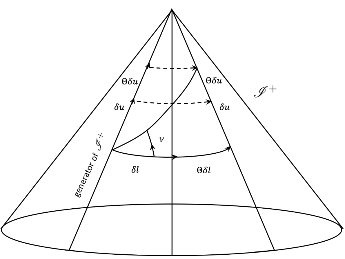
In virtue of the strong conformal geometry, under change of the conformal factor for the metric of , null angles
remain invariant. For further insights about the strong conformal geometry and the interpretation of null angles we suggest to read Penrose (1972a) or Schmidt et al. (1975).
A transformation of to itself which
preserves angles and null angles, i.e. that respects the strong conformal geometry structure, must have
the effect that any expansion (or contraction) of the spatial distances is accompanied by an equal
expansion (or contraction) of the scaling of the special parameters. The allowed transformations
have the form (6.4.8a), where function must now have the precise form that allows the ratio
to remain invariant. Under the transformation (6.4.9) we have, as seen, that the sphere
of the cross-section of undergoes a conformal mapping, i.e.
Since is the conformal factor of the transformation, it depends only on and or, equivalently, on and and must have the form given in (6.4.7). We must therefore also have
Integrating we get
where assumes the form
with and . In virtue of definition 6.3.1 we have obtained the following
Proposition 6.4.2.
The group of conformal transformations of which preserve the strong conformal geometry, i.e. both angles and null angles, is the BMS group.
Remark 6.4.3.
Conformal transformations, and hence the NU group, always preserve finite angles, but null angles, i.e. angles between tangent vectors of which is a linear combination, are preserved by the BMS group only.
The general form of a BMS transformation is thus
| (6.4.15a) | |||
| (6.4.15b) |
with and . Clearly the BMS group is a subgroup of the NU group, the function having its form fixed. However it is still an infinite-dimensional function-space group.
6.5 Structure of the BMS Group
We discuss first the BMS transformations obtained by setting ,
| (6.5.1) |
with
i.e. a rescaling for and a transformation of the group for . Any of these transformations is specified by the 4 constants , satisfying . Hence there are only 3 independent complex parameters, i.e. 6 independent real parameters. Any element reads as
Note that under simultaneous change , , , any element remains unaffected, i.e.
| (6.5.2) |
Now take into account the group of complex matrices with :
Clearly the dimension of is 6. Hence we can consider a map , between and defined by
| (6.5.3) |
It is easy to show that, since the group operation of is the function composition , given and we have
Then taking the images of and through ,
we have, since the operation in is the ordinary matrix product,
| (6.5.4) |
Note that, in virtue of (6.5.2), to the same element there correspond, through , two different elements, and . If we consider now the map :
it is clear that property (6.5.4) holds for as well. This map is a group isomorphism, and being now identified in . We can state
| (6.5.5) |
The group is the double covering of . As already pointed out in the introduction of chapter 2, we also have
| (6.5.6) |
where is the connected component of the Lorentz group. Thus
| (6.5.7) |
We have the following
Proposition 6.5.1.
The connected component of the Lorentz group is isomorphic with the subgroup of the BMS group.
To make this isomorphism explicit take an element and through assign it an element of ,
Then, using the isomorphism of (6.5.6) it can be shown with tedious calculations (Oblak, 2016b) that to there corresponds an element of through the isomorphism of (2.1.5):
| (6.5.8) |
At this stage, the relation between the Lorentz group and the sphere appears as a mere coincidence. In particular, since the original Lorentz group is defined by its linear action on a four-dimensional space, there is no reason for it to have anything to do with certain non-linear transformations of a two-dimensional manifold such as the sphere. However, it can be shown that it is not accidental. Following Oblak (2016b), we can suppose to perform a Lorentz transformation in Minkowski space-time equipped with standard coordinates , i.e.
We may introduce Bondi coordinates for Minkowski space-time as done in (6.2.1). Then if we evaluate the limit for large values of the radial coordinate keeping the value of fixed (i.e. on ) and use the isomorphism (6.5.6) and hence (6.5.8) we obtain the following behaviour:
where
. Furthermore it can be checked that both and , under
the effect of a Lorentz transformation on , undergo an angle-dependent rescaling. Hence
we have obtained a fundamental result: Lorentz transformations acting on , expressed in
terms of the parameters coincide with conformal transformations of .
Since asymptotically flat space-times have the same structure of a Minkowski space-time at infinity,
this argument can be extended to all of them too. In the remainder we will use to describe
the group structure of , the isomorphism with being implicit.
Now we turn to analyse the transformations which involve a non-vanishing .
Definition 6.5.1.
The Abelian subgroup of BMS transformations for which
| (6.5.9) |
is called supertranslations subgroup and is denoted by .
Under such a transformation the system of null hypersurfaces is transformed into another
system of null hypersurfaces .
To proceed further in the analysis of the structure of the BMS group we need to recall the concepts of
right and left cosets and, hence, that of normal subgroup Curzio et al. (2014).
Consider a group and a subgroup of . Introduce in the equivalence relation
defined, for , , as
It is easy to verify that the previous relation is reflexive, symmetric and transitive.
Definition 6.5.2.
The equivalence class with respect to is called right coset of in with respect to and is denoted by :
Similarly, the left coset of in with respect to can be introduced as
Generally, the right and the left cosets are different sets.
Definition 6.5.3.
A subgroup of which defines a unique partition,
is called normal subgroup of .
Clearly it follows that for every and the product . Note that every group
possesses normal subgroups, since and the identity are normal subgroups.
Now consider for a general subgroup of the quotient group (or factor group) , defined as
If is normal the elements of are, indistinctly, the right and left cosets. Furthermore, under this hypothesis, the set can be equipped with a group structure in a natural way by defining the product :
i.e.,
It can be shown that equipped with the product satisfies the group axioms. We are now ready to
discuss further the BMS properties.
Any element of can be written as
Note that with this nomenclature any element of (or, equivalently, of
) can be written as and any element of
as , where denotes the identity in .
The action of on the variables is
where is the element of which corresponds to through the above
discussed isomorphism and its conformal factor.
It is easy to show that, with this notation, we have for the inverse of :
| (6.5.10) |
Considering an element of we have
with
From the above discussion we have the following
Proposition 6.5.2.
The supertranslations form an Abelian normal, infinite-parameter, subgroup of the BMS group:
Under the assumption that the function is twice differentiable, we can expand it into spherical harmonics as
| (6.5.11) |
Definition 6.5.4.
If in decomposition (6.5.11) for , i.e.
| (6.5.12) |
then the supertranslations reduce to a special case, called translation subgroup, denoted by , with just four independent parameters .
It is easy to show that implies
Then equation (6.5.12) becomes
with and real. Hence in terms of and a translation is
If we let be Cartesian coordinates in Minkowski space-time, it is easy to see that
where . Now if we perform a translation
it is easy to get
with , and . Thus, the nomenclature ‘translation’ is consistent
with that for the space-time translations in Minkowski space-time. In fact we have just shown that any
translation in the ordinary sense induces a translation (i.e. an element of ) on .
It is easy to verify that for any and for any
we have
with
Note that it is not obvious that is still a function of and containing only zeroth- and first-order harmonics. A proof of this result will be given in section 6.7. Taking for the moment this result for true it follows that:
Proposition 6.5.3.
The translations form a normal four-dimensional subgroup of :
and clearly
We have the following inclusion relations:
The next step will be to investigate the group structure of . It is easy to show that for any there exists a unique and such that . In fact given
we have that
with . The uniqueness results from the observation that where is the identity in , since if , then implying and . Hence we have
| (6.5.13) |
Furthermore, the supertranslations form an (Abelian) normal subgroup of , according to 6.5.2. Thus we can already state that, by definition of semi-direct product,
Proposition 6.5.4.
The BMS group is a semi-direct product of the conformal group of the unit -sphere with the supertranslations group, i.e.
We can say more by specifying an action of on and, hence, by specifying a product rule for two elements of . Let be the vector space of real functions on the Riemann sphere. Let be a smooth right action of on defined as
| (6.5.14a) | |||
| such that | |||
| (6.5.14b) | |||
where is the conformal factor associated with , the element of that corresponds to . Then it is easy to verify that the composition law for the elements of is
Note that the inverse of in (6.5.10) may be written as
Thus the BMS group is the right semi-direct product Colombo and Jacobs (2014) of with under the action , i.e.
| (6.5.15) |
Historically, this semi-direct product structure was realized by Cantoni (1966). Succesively this idea was developed
by Geroch and Newman (1970) who gave an incorrect formula for the action (6.5.14). Eventually the mistake was amended
by McCarthy (1973), who defined a good action to describe the semi-direct product structure of the BMS group.
However, the idea used here of giving a right action and hence of describing the BMS group as a right
semi-direct product was not developed by any of these authors.
Furthermore, it can be shown that from the above discussion it follows that, by virtue
of the first isomorphism theorem,
| (6.5.16) |
i.e. is the factor group of with respect to its normal subgroup .
Remark 6.5.1.
Note that the structure of the BMS group is similar to that of Poincaré group, denoted by . In fact the Poincaré group can be expressed as the semi-direct product of the connected component of the Lorentz group and the translations group , the former being the factor group of with respect to the latter, i.e. . The action of on is the ‘natural’ one, i.e. the usual multiplication of an element with a vector .
Theorem 6.5.1.
If is a 4-dimensional normal subgroup of , then is contained in .
Proof.
Consider the image of under the homomorphism . Since by hypothesis is a normal subgroup of , is a normal subgroup of and hence, by proposition 6.5.2, a subgroup of the connected component of the Lorentz group . However, the only normal subgroups of are itself and the identity of . Then must be -dimensional, contrary to hypothesis. Therefore ; is thus contained in . ∎
6.6 BMS Lie Algebra
In this section we are going to investigate the Lie Algebra of the BMS group. At first we consider the generators of of (6.5.1). For an infinitesimal conformal transformation we know that the coordinates change as
where is a conformal Killing vector of (6.3.16) of the unit 2-sphere. Furthermore, from (6.5.1) and taking into account (6.3.18d) an infinitesimal transformation for reads as
Thus, the generator of transformation (6.5.1) is
| (6.6.1) |
To see how their Lie algebra closes consider the Lie brackets of two of them, and :
After some calculation the term proportional to becomes
The last term in the previous equation vanishes since it can be shown by direct calculation that for the metric
and hence
Finally we get
| (6.6.2a) | |||
| where | |||
| (6.6.2b) | |||
We take now into account the generators of supertranslations. It is clear from (6.5.9) that these are
where is an arbitrary function of and . It follows that the Lie brackets of two generators, and vanish, i.e.
| (6.6.3) |
that is just a restatement that the supertranslations group is Abelian. The only thing left to do is to calculate the Lie brackets of and . It is easy to see that
| (6.6.4a) | |||
| where | |||
| (6.6.4b) | |||
If we consider now as defined in (6.3.17) it turns out . From the above discussions one obtains that
| (6.6.5) | |||||
with
To sum up the Lie algebra of the BMS group, , is
Since, as shown in the previous section, the BMS group is a semi-direct product, it follows that the BMS Lie algebra, , should be taken to be the semi-direct sum of the Lie algebra of conformal Killing vectors of the Riemann sphere, denoted by (since it can be taken to be the algebra of ) with that of the functions on the Riemann sphere, which we denote by , the supertranslations group being Abelian. Given an element ( being a generator of conformal transformations in (6.3.16)) we know that the exponential map associated to it, , is an element of . Then consider the 1-parameter group of transformations in defined as
| (6.6.6) |
where is that of (6.5.14). Consider the map
such that
Note that is the infinitesimal generator of (6.6.6). Hence Oblak (2016a) we have
| (6.6.7) |
The Lie algebra is determined by three arbitrary functions and on the circle. Thus, defining and labelling elements of (6.6.7) as pairs , we know that the Lie brackets in are
| (6.6.8) |
Equation (6.6.8) follows from the fact the is Abelian, otherwise there would be an extra term involving the commutator of the two elements and . Since we have, using (6.5.14) and (6.3.18d)
then (6.6.8) may be written as
| (6.6.9a) | |||
| with | |||
| (6.6.9b) | |||
as remarked in Barnich and Troessaert (2010b); Barnich and Troessaert (2010a).
Remark 6.6.1.
Depending on the space of functions under consideration, there are many options which define what is actually
meant by . The approach that will be followed in this work is originally due to
Sachs (1962a) and successively amended by Antoniou and Misra (1991). Another approach, based on the Virasoro algebra,
can be found in Barnich and Troessaert (2010b).
In general, we consider any -dimensional Lie transformation group of a -dimensional space. Let
the coordinates of the space be and the parameters of the group be
, where is the identity of the group. Then the transformations have the form
The functions are assumed to be twice differentiable. The generators of the group are the vector fields given by
| (6.6.10) |
Applying these ideas to the BMS group, with the Sachs’s notations Sachs (1962a), it gives for the supertranslations, using the expansion (6.5.11):
and hence
i.e. two supertranslations commute.
To find the generators of conformal transformations we have to be careful. We know that any conformal
transformation has the form
By direct calculations one obtains that the following equations hold for , and :
| (6.6.11a) | ||||
| (6.6.11b) | ||||
| (6.6.11c) | ||||
On denoting by the parameter of the transformation it is clear that are functions of such that and . We have to apply (6.6.10) to (6.6.11). It is easy to verify that
These equations hold in general for any conformal transformation. We choose now to work with Lorentz transformations, and thus to use Lorentz generators and of rotations and boosts, respectively. To know the coefficients corresponding to a Lorentz transformation we need to use the isomorphism (6.5.6). Any rotation of an angle about an axis and any boost of rapidity about an axis can be done by using a matrix given by
| (6.6.12a) | ||||
| (6.6.12b) | ||||
respectively, where are the Pauli matrices of (2.1.2). The parameter of the two transformations is and , respectively. After some calculations we find that the vector fields that generate the transformations are
| (6.6.13) | ||||
| (6.6.14) | ||||
| (6.6.15) | ||||
| (6.6.16) | ||||
| (6.6.17) | ||||
| (6.6.18) |
Note that rotations are characterized by . The and form a complete set of linearly independent vector fields for the Lie algebra . We can find now the commutators
where and is the Levi-Civita symbol. Note that we have just obtained the classical Lorentz algebra. Furthermore, it is easy to derive the following commutator:
| (6.6.19) |
where is defined by the relation
for arbitrary .
For convenience we introduce the raising and lowering operators,
in terms of which, using equation (6.6.19), we give the commutation relations with the generators of the supertranslations:
The form of the commutation relations shows that the BMS algebra is the semi-direct sum of the Lorentz algebra with the infinite Lie algebra , as remarked before.
6.7 Good and Bad Cuts
We begin this section by citing a remarkable result obtained by Sachs.
Theorem 6.7.1.
Sachs (1962a) The only -dimensional normal subgroup of the BMS group is the translation group.
Theorem 6.7.1 characterizes translations uniquely: the translations normal subgroup of the BMS group
is singled out by its group-theoretic properties. Since we have shown that the translations are
the BMS transformations induced on by translations in Minkowski space-time, theorem
6.7.1 makes it possible for us to define the asymptotic translations
of a general asymptotically flat space-time
as the BMS elements belonging to this normal subgroup. However a similar procedure for ,
i.e. rotations and boosts, fails. Thus, as we will discuss in this section, there are several problems in
identifying the Poincaré group as a subgroup of .
The Poincaré group is the symmetry group of flat space-time, hence it might have been thought that a suitably
asymptotically flat space-time should, in some appropriate sense, have the Poincaré group as an asymptotic
symmetry group. Instead, it turns out that in general we seem only to obtain the BMS group (which has
the unpleasant feature of being an infinite-dimensional group) as the asymptotic symmetry group of an
asymptotically flat space-time.
To better understand the nature of this problem we revert to Minkowski space-time and see how the Poincaré
group arises in that case as a subgroup of the BMS group. The BMS group was defined as the group of
transformations which conformally preserves the induced metric on and the strong conformal
geometry. However, the BMS group is much larger than the Poincaré group and thus the former must preserve
less structure on than does the latter. The preservation of this additional structure,
in the case of Minkowski space-time, should allow us to restrict the BMS transformations to Poincaré
transformations, since we know that in that case is a subgroup of .
In Minkowski space-time a null hypersurface is said to be a good cone if it is the future light cone
of some point, and a bad cone if its generators do not meet at a point. Consequently we define a
good cross-section, often called a good cut, a cross-section of which is
the intersection of a future light cone of some point and the null hypersurface .
A bad cut is, on the other hand, the intersection of with some null hypersurface
which does not come together cleanly at a single vertex. The situation is reported in Figure 6.4.

Using Bondi-Sachs coordinates the Minkowski metric tensor takes the form
We see that each cut of given by is a good cut, since it arises from the future light cone of a point on the origin-axis . In particular, all the good cuts can be obtained from the one given by by means of a space-time translation. Hence, as discussed in section 6.5 we obtain that every good cut can be expressed in the form
| (6.7.1) |
being real and being complex. Hence the equations describing good cuts are given, generally,
by setting equal to a function of and which consists only of zeroth-
and first-order spherical harmonics.
The effect of a transformation of the connected component of the Lorentz group is to leave invariant the
particular good cut . Such a transformation is
| (6.7.2a) | ||||
| (6.7.2b) | ||||
with such that . Note that transformations (6.7.2) preserve the functional form of good cuts given in (6.7.1). In fact we have, applying (6.7.2), that
where and have now to be expressed as functions of and . It is straightforward to show that
where
For example, if we perform a boost in the direction we have from (6.6.12)
. Hence we get .
Now it is clear that the general BMS transformation which maps good cuts into good cuts must obtain the particular
good cut from some other good cut. We can therefore express the BMS transformation as the composition
of a translation which maps this other good cut into , with a Lorentz transformation which leaves
invariant. Thus, the BMS transformation is
| (6.7.3a) | ||||
| (6.7.3b) | ||||
These BMS transformations form a -real-parameters group. This is exactly the Poincaré group of Minkowski space-time, being a composition of a Lorentz transformation and a translation. We have obtained the following
Proposition 6.7.1.
The Poincaré group is the group of transformations which maps good cuts into good cuts in Minkowski space-time.
However, there are many other subgroups of the BMS group which can be expressed in the form (6.7.3) and which are therefore isomorphic with the Poincaré group. In fact is not a normal subgroup of the BMS group since for any and for any the product is not necessarily an element of , as can be easily verified, and hence does not get canonically singled out, occurring only as a factor group of by the infinite-parameter Abelian group of supertranslations . In particular, Lorentz transformations do not commute with supertranslations and if we take any supertranslation and consider the group then it is a subgroup of the BMS group which is distinct from but still isomorphic, and thus equivalent, to it. Explicitly, having fixed a supertranslation , a transformation of reads as
| (6.7.4a) | ||||
| (6.7.4b) | ||||
If we start with the good cut described by the equation , which is left invariant by , and
perform the supertranslation , we obtain a new (bad) cut given by . This is the cut which is left
invariant by (6.7.4) and hence by . Hence maps bad cuts into bad cuts.
It follows that if we conjugate the whole Poincaré group of (6.7.3) with respect to
any supertranslation which is not a translation obtaining we get a
distinct subgroup of , but isomorphic and completely equivalent to , which maps
bad cuts into bad cuts. Of course, for a general , and have only the
translations in common. There exist many subgroups of which are
isomorphic with and hence the Poincaré group is not a subgroup of the BMS group
in a canonical way. However we have just seen that in Minkowski space-time, if we require the group of
transformations to preserve the conformal nature of and the strong conformal geometry, together
with the property of mapping good cuts into good cuts, just one of the several copies of the
Poincaré group gets singled out.
Remark 6.7.1.
Note that, again, the situation is similar to what happens for within . In fact does not arise naturally as a subgroup of , since if we form the group , where is a translation, it is a different subgroup of but isomorphic to . We can say, since the commutator of a Lorentz transformation and a translation is a translation, that , as a subgroup of , depends on the choice of an arbitrary origin in Minkowski space-time.
We turn now to the case when the space-time is asymptotically flat. The difficulty here is that there seems
to be no suitable family of cuts that can properly take over the role of Minkowskian good cuts. This means
that, although the translation elements of are canonically singled out, there is no canonical
concept of a ‘supertranslation-free’ Lorentz transformation. Hence the notion of a
‘pure translation’ still makes sense, but that of ‘pure rotation’
or ‘pure boost’ does not.
The most obvious generalization, for an asymptotically flat space-time, of the Minkowskian definition
of a good cut, i.e. the intersection of future light cone of a point with , is totally
inappropriate. One first reason is that there are many perfectly reasonable asymptotically flat space-times
in which no cuts of at all would arise in this way, e.g. Penrose (1972a). Even if we
restrict attention only to asymptotically flat space-times which do contain a reasonable number of good cuts
of this kind, we are not likely to obtain any of the BMS transformations (apart from the identity) which
maps this system of cuts into itself. The difficulty lies in the fact that the detailed irregularities of
the interior of the space-time would be reflected in the definition of ‘goodness’
of a cut. In other words, the light-cone cuts are far more complicated than those (6.7.1) of flat space.
However there is a more satisfactory way to characterize good cuts of , based on the shear (see section 2.8) of null hypersurfaces intersecting . Consider now that the (physical) space-time under consideration contains a null curve of a null geodesics congruence affinely parametrized by and whose tangent null vector is . Complete to a spin basis at a point of . We can propagate and along via
where . From the results of section 2.8 we have that . From the first two equations Newman-Penrose field equations in Appendix B we obtain for the shear and for the divergence the so-called optical equations of Sachs (Sachs, 1961; Sachs, 1962b):
| (6.7.5a) | ||||
| (6.7.5b) | ||||
Introducing the matrices
then, equations (6.7.5) may be written as
| (6.7.6) |
Consider first the case of a flat space-time, i.e. . Then equation (6.7.6) reduces to
where I is the () unit matrix. But
hence we obtain
where and is affine along the congruence, i.e. .
Writing
where and are the values of and at , we get, explicitly
| (6.7.7a) | |||
| (6.7.7b) | |||
Thus has the following asymptotic behaviour:
where is called asymptotic shear. Note that in a flat space-time the vanishing of the asymptotic shear implies the vanishing of the whole shear. If we now turn to the case of asymptotically flat space-times with non-vanishing and , it can be shown, in virtue of their asymptotic behaviours, that the leading term of the asymptotic behaviour of does not change. However the vanishing of does not, in this non-flat case, imply that vanishes (Adamo et al., 2012).
Note that, in virtue of thorem 2.8.1, if we consider the unphysical space-time obtained with conformal factor the shear transforms as
In Minkowski space-time the good cones are characterized locally by the fact that the null rays generating them possess no shear and it can be shown that the cuts of which we defined earlier are precisely the ones arising from the intersection of with null hypersurfaces characterized by . Thus a definition of ‘goodness’ is provided, for Minkowski space-time, which refers only to quantities defined asymptotically.
We would like to extend this definition of good cut to asymptotically flat space-times too. To do that all we need to do is to set up and (see section 2.3) at each point of the cut at , where is complex null, with real and imaginary parts both tangent to the cut and where is real null and orthogonal to , i.e. . The cut is a good cut if the complex shear so obtained equals zero (since on we have ).
We cannot, however, define good cones simply by requiring . In many cases it is not possible to arrange for all values of and . But even in cases where it is possible we have another problem, which is due to the presence of gravitational radiation. To make this point clear, we cite now some important results regarding the relation between asymptotic shear and gravitational radiation which are basically due to Bondi et al. (1962); Newman and Unti (1962); Sachs (1962b). At first forms part of the initial data on used to determine the space-time asymptotically. We introduce the Bondi news function :
Clearly, need not vanish near even though does. It turns out that
where is the (complex conjugate) gravitational radiation field introduced in section 5.5. The news function enters in the Bondi-Sachs definition of mass-momentum. In fact let us consider a hypersurface which spans some two-dimensional cross-section of . That is to say, . The total energy-momentum intercepted by is equal to the following integral over .
where
Note that, is topologically a sphere and can always be transformed, by the introduction of a suitable conformal factor into a metric sphere of unit radius. Hence can be taken to be
Thus, the Bondi mass (see section 3.1) at a cut is
The rate of energy-momentum loss due to gravitational radiation is
| (6.7.8) |

Thus, the squared modulus of represents the flux of energy-momentum of the outgoing gravitational radiation. The time component of (6.7.8) gives the famous Bondi-Sachs mass-loss formula:
| (6.7.9) |
The positivity of the integrand in (6.7.9) shows that if a system emits gravitational waves, i.e. if there is news, then its Bondi mass must decrease. If there is no news, i.e. , the Bondi mass is constant. The reason we get a mass loss rather than a mass gain is simply that the above discussion has been applied to instead of .
From the above discussion it follows that, if the cut is given by and is shear-free, the cross-sections , which are translations of , will not be shear-free in the presence of gravitational radiation. In other words, if for one value of , we will generally have for a later value of , i.e. ‘goodness’ would not be invariant under translation. However, there is a more serious difficulty even than this. Since to specify a cut we just need to specify the value of on each generator of , the freedom in choosing a cut is one real number per point of the cut. On the other hand the quantity is complex, its vanishing therefore, representing two real numbers per point of the section. To solve this problem we need to define the magnetic and the electric part of . Under a rotation of the spacelike vectors , in their plane, given by
| (6.7.10) |
we have, from the definition of shear,
| (6.7.11) |
We say that has spin weight 2. Furthermore it can be shown (Sachs, 1962b) that, under a BMS transformation for which , i.e. a conformal transformation, we have
| (6.7.12) |
Thus we say that has conformal weight . Generally we give the following
Definition 6.7.1.
A scalar will be said to have spin weight if it transforms as
under (6.7.10) and a conformal weight if it transforms under BMS conformal transformations as
We define the differential operator (Goldberg et al., 1967; Penrose and Rindler, 1984) acting on a scalar of spin weight , in the particular coordinate system :
It is easily seen that, under (6.7.10), we have
i.e. raises the spin weight by 1. Similarly lowers the spin weight by 1. We also have
We can define spin- spherical harmonics for integral and by
where are ordinary spherical harmonics. Note that are not defined for . It can be shown that the form a complete orthonormal set for each value of , i.e. any function of spin weight can be expanded in a series in . If we pass now to complex stereographic coordinates , we have that
with . The spin- spherical harmonics take now the form
We have
In particular we see from the above relations that annihilates whenever and annihilates when if . Furthermore the are eigenfunctions of for each spin weight . If , is essentially the total angular momentum.
We give now three important results, whose proof can be found in (Newman and Penrose, 1966).
Theorem 6.7.2.
The operator is invariant, with spin weight unity, under change of coordinate system which preserves the sphere metric
i.e., under we have .
Theorem 6.7.3.
Let have conformal weight and spin weight , where . Then is a quantity of conformal weight and of spin weight . Furthermore we have for the commutator
Theorem 6.7.4.
Given any suitably regular on the sphere of spin weight , there exists of spin weight zero for which
Using theorem 6.7.4, for a quantity of spin weight on the sphere, we can define its electric and magnetic part, denoted by and respectively, given by
such that
with (see theorem 6.7.3)
The invariance properties of imply that the concepts of magnetic and electric parts of are invariant under rotations of the sphere or of the vectors. Furthermore, in virtue of theorem 6.7.3, only if has conformal weight , does the split of onto its electric and magnetic parts turn out to be invariant also under BMS conformal transformations.
We apply now these concepts to which has and . Thus, for each hypersurface we have a splitting , which is invariant under Lorentz transformations, which leave the surface invariant.
Now, it can be shown (Newman and Penrose, 1966) that in the Minkowski case, the asymptotic shear behaves, when as
| (6.7.13a) | ||||
| (6.7.13b) | ||||
with purely electric and independent of . The magnetic part , as vanishes, i.e. .
On the basis of what happens in the Minkowski case we wish to impose a physical restriction on the behaviour of as for a general space-time. Although no actual cuts of may be shear-free, it is reasonable to expect that in the limit on , such cuts will exist. Requiring that this limiting shear-free cuts be sent into one another, we can actually restrict the BMS transformations to obtain a canonically defined subgroup of the BMS group, which is isomorphic to the Poincaré group. The Poincaré group which emerges in this way, in virtue of the considerations we have done on the gravitational radiation, may be thought of as that which has relevance to the remote past, before all the gravitational radiation has been emitted. In analogy with (6.7.13) we require that
| (6.7.14) |
If the analogy with the Minkowski theory is to be trusted, we would expect to be purely electric. However, it is not essential since it will be possible to extract the Poincaré group only on the basis of (6.7.14). Hence we will treat the case in which could have a magnetic part too, i.e. with .
It can be shown (Sachs, 1962b) that, under a full BMS transformation, the asymptotic shear transforms as
| (6.7.15) |
It has to be remarked that refers to the asymptotic shear of the hypersurface of the transformed coordinate system evaluated at . The complete transformation is more complicated. Applying (6.7.14) to (6.7.15) gives
since is real. Using theorem 6.7.4 we can set
for some real . Since can be chosen arbitrarily on the sphere, it follows that a BMS transformations for which imposes . Thus we have introduced coordinate conditions for which at . Now the BMS transformations which preserve the condition are those for which
It can be easily shown that this condition restricts to be of the form of (6.5.12) and thus the allowed supertranslations are simply the translations. The Lorentz transformations, given by do not spoil the coordinate conventions. We have finally obtained the following
Theorem 6.7.5.
The group of asymptotic isometries of an asymptotically flat space-time which preserves the condition at is isomorphic with the Poincaré group .
Remark 6.7.2.
We could have carried out the same arguments by taking the limit , and it would have been an independent choice. Thus, in a similar way, we could have extracted another Poincaré group which has relevance to the remote future, i.e. after all the gravitational radiation has been emitted. There seems to be no reason to believe that these two Poincaré groups will be the same, in general.
6.8 Applications of the BMS Group
There are many very recent applications of the BMS formalism and of particular interest are the ones that have to do with black-hole physics in quantum gravity. Maybe the most significant of them is the one which is due to Strominger (2014). In this work, the author identifies the two different copies of the BMS group of and of as and , respectively. Starting from the idea that and act non-trivially on outgoing and ingoing gravitational scattering data, it is argued that in Christodoulou-Klainerman space-times (Christodoulou and Klainerman, 1993) it is possible to make a canonical identification between the generators and of and (using the link between and ), and hence to find what are called the ‘diagonal’ generators of . Then, since in asymptotically flat quantum gravity one seeks an -matrix relating the ‘in’ and ‘out’ Hilbert states, i.e.
it is asked whether or not the BMS group could provide a symmetry of the -matrix and it is guessed a relation of the form
The classical limit of such a relation would give symmetries of classical gravitational scattering. The generators are made up of Lorentz generators, which provide the usual Lorentz invariance of the -matrix, and of the supertranslations generators which provide that the local energy is conserved at each angle. In fact the simple translations, that are supertranslations whose magnitude does not depend on the angle or position on , lead, as known, to global energy conservation. Then it is plausible that the supertranslations which act at only one angle lead to the conservation of energy at that one angle. Furthermore in quantum theory, matrix elements of the conservation laws give an infinite number of exact relations between scattering amplitudes in quantum gravity. These relations turned out (He et al., 2015) to have been previously discovered by Weinberg (1965) using Feynman diagrammatics and are known as the soft graviton theorem.
The results obtained by Strominger paved the way for a deeper investigation of the so called ‘soft hair’ of black holes. In Hawking et al. (2016a) the authors showed that the Minkowski vacuum in quantum gravity is not invariant under supertranslations. In particular such transformations map the Minkowski vacuum into a physically inequivalent zero-energy one. Hence, the supertranslation symmetry is spontaneously broken and the ‘soft’ (i.e. zero-energy) gravitons are the associated Goldstone bosons. Since the information paradox (Hawking, 1975; Hawking, 1976) relies on the fact that the vacuum is unique, this would be a motivation to doubt of its validity. Furthermore, the information loss argument assumes the fact that the black holes are only characterized by their mass , charge and angular momentum . But supertranslations map a stationary black hole to a physically inequivalent one and in the process of Hawking evaporation, supertranslation charge will be radiated through null infinity. Since this charge is conserved, the sum of the black hole and radiated supertranslation charge is fixed at all times. This requires that black holes carry soft hair (i.e. additional data, besides mass, charge and angular momentum) arising from supertranslations. Moreover, when the black hole has fully evaporated, the net supertranslation charge in the outgoing radiation must be conserved. This leads in turn to correlations between the early- and late-time Hawking radiation. In Hawking et al. (2016b) the same authors showed that black holes in General Relativity are characterized by an infinite head of supertranslation hair and that distinct black holes are characterized by different classical superrotation charges measured at infinity.
Appendix A Topological spaces
Definition A.0.1.
A topological space consists of a set together with a collection of subsets of satisfying the following three properties:
- •
The union of an arbitrary collection of subsets, each of which is in , is in , i.e. if for all , then ;
- •
The intersection of a finite number of subsets in is in , i.e. if then
- •
The entire set and the empty set are in .
Usually is referred to as topology on , and subsets of which are listed in the collection are called open sets.
Let and be topological spaces and a map between them.
Definition A.0.2.
is said to be continuous if the inverse image, , of every open set in is an open set in .
Definition A.0.3.
If is continuous, one-to-one, onto and its inverse is continuous, is called a homomorphism and and are said to be homeomorphic.
Definition A.0.4.
If is a topological space, a subset of is said to be closed if its complement is open.
Note that a subset may be neither open nor closed or may be both open and closed. This last possibility gives rise to the definition of connectedness.
Definition A.0.5.
A topological space is said to be connected if the only subsets which are both open and closed are and .
Consider a topological space and an arbitrary subset of , say .
Definition A.0.6.
The closure of , , is defined as the intersection of all closed sets containing .
Obviously is closed, contains and equals if and only if is closed.
Definition A.0.7.
The interior of , , is defined as the intersection of all open sets contained within .
Clearly is open, is contained in and equals if and only if is open.
Definition A.0.8.
The boundary of , , consists of all points which lie in but not in :
Definition A.0.9.
A topological space is said to be Hausdorff if for each pair of distinct points , , , one can find open sets , such that and , and .
Let be a topological space, be a collection of open sets and a subset of .
Definition A.0.10.
is said to be a open cover of if the union of these sets contains .
Definition A.0.11.
A subcollection of the sets which also covers is referred to a subcover.
The two previous definitions allow us to give the following
Definition A.0.12.
The set is said to be compact if every open cover of has a finite subcover, i.e. a subcover consisting of only a finite number of sets.
The general relation between compact and closed sets is described by the following two theorems.
Theorem A.0.1.
Let be Hausdorff and let be compact. Then is closed.
Theorem A.0.2.
Let be compact and let be closed. Then is compact.
We need now to give the notion of convergence of sequences.
Definition A.0.13.
A sequence of points in a topological space is said to converge to point if given any open neighbourhood of (i.e. an open set containing ) there is an such that for all . The point is said to be the limit of this sequence.
Definition A.0.14.
A point is said to be an accumulation point of if every open neighbourhood of contains infinitely many points of the sequence.
It follows that if converges to , then is an accumulation point of the sequence. However, in a general topological space, if is an accumulation point of it may not even be possible to find a subsequence of the sequence which converges to . Hence we give the following
Definition A.0.15.
A topological space is first countable if for each there is a countable collection of open sets such that every open neighbourhood, , of contains at least one member of this collection.
A stronger requirement is the following
Definition A.0.16.
A topological space is second countable if for each there is a countable collection of open sets such that every open neighbourhood, , of can be expressed as a union of sets in the collection.
The Bolzano-Weierstrass theorem expresses the important relation between compactness and convergence of sequences.
Theorem A.0.3.
Bolzano-Weierstrass Let be a topological space and let . If is compact then every sequence of points in has an accumulation point lying in . Conversely if is second countable and every sequence of points in has an accumulation point in , then is compact. Thus in particular, if is second countable, is compact if and only if every subsequence in has a convergent subsequence whose limit lies in .
We give now the definition of paracompactness. Let be a topological space and let be an open cover of .
Definition A.0.17.
An open cover is said to be a refinement of if for each there exists an such that .
Definition A.0.18.
The cover is said to be locally finite if each has an open neighbourhood such that only finitely many satisfy .
Definition A.0.19.
A topological space is said to be paracompact if every open cover of has a locally finite refinement .
We can now give the definition of a manifold.
Definition A.0.20.
A -dimensional topological manifold is a topological space with a collection of open subsets of , such that
- •
is an open cover of , i.e. ;
- •
For each , there is a one-to-one, onto, homomorphism , where is an open subset of ;
Remark A.0.1.
Usually the pair is called chart or coordinate system and the collection is called atlas. If we can consider the map which takes points in to points in . This map is an homomorphism and is often called coordinate change.
Consider now two topological manifolds and , with respective dimensions and , and a map between them. Let and be respectively charts of and .
Definition A.0.21.
is said to be if the map is in the sense of usual differential calculus.
Let now be an homomorphism, between and .
Definition A.0.22.
is said to be a diffeomorphism if is with its inverse (i.e. the map ).
We can now give the definition of differentiable manifold.
Definition A.0.23.
A -dimensional differentiable manifold is a topological manifold such that all the coordinate changes are maps with their inverses of into itself.
Remark A.0.2.
It is clear that for a differentiable manifold all the coordinate changes must be diffeomorphisms of into itself.

Before we state some important theorems about manifolds we want to briefly comment manifolds-with-boundary without going into details. It is remarkable that the boundary of a manifold is not defined to be the boundary of the topological space . If is covered by a family of open sets , suppose that some of them is homeomorphic not to , but to an open set of ( is called Euclidean half-space). Then the set of points which are mapped to points with is called the boundary of and is denoted by . The coordinates of may be given by numbers . A Further details about the smoothness of coordinate changes and examples can be found in Lang (2002), in Nakahara (2003) or Spivak (1999).
Consider now a paracompact manifold , i.e. a manifold whose topological space is paracompact.
Theorem A.0.4.
A paracompact manifold is second countable.
Corollary A.0.1.
A paracompact manifold can be covered by a locally finite, countable family of charts with each compact.
Consider a locally finite cover of .
Definition A.0.24.
A partition of unity subordinate to is a collection of smooth functions such that
- 1.
the support of is contained within ;
- 2.
;
- 3.
.
Theorem A.0.5.
Every locally finite open cover of a paracompact manifold , such that is compact, admits a subordinate partition of unity.
Corollary A.0.2.
Using this theorem we can define a local Riemannian metric on each and build a Riemannian metric defined all through by setting .
The proof of the last two theorems can be found in Kobayashi and Nomizu (1963).
Theorem A.0.6.
Let be a manifold which is locally compact Haussdorff and whose topology has a countable basis. Then is paracompact.
The proof and insights of this theorem can be found in Lang (2002) or in Engelking (1989).
Appendix B The Newman-Penrose formalism
The source-free Maxwell equations in the Newman-Penrose formalism are:
- 1.
;
- 2.
;
- 3.
;
- 4.
.
The Newman-Penrose field equations are:
- 1.
- 2.
- 3.
- 4.
- 5.
;
- 6.
- 7.
- 8.
- 9.
- 10.
- 11.
- 12.
- 13.
- 14.
- 15.
- 16.
- 17.
- 18.
Appendix C Christoffel Symbols
References
- Adamo et al. (2012) Adamo, T. M., Newman, E. T., and Kozameh, C. (2012). Null Geodesic Congruences, Asymptotically-Flat Spacetimes and Their Physical Interpretation. arXiv:0906.2155v3.
- Antoniou and Misra (1991) Antoniou, I. E. and Misra, B. (1991). Characterization of semidirect sum Lie algebras . J. Math. Phys., 32:864–868.
- Avez (1963) Avez, A. (1963). Essais de géometrie Riemannienne hyperbolique globale. Applications à la Relativité Générale. Ann. Inst. Fourier (Grenoble), 132:105–190.
- Barnich and Troessaert (2010a) Barnich, G. and Troessaert, C. (2010a). Aspects of the BMS/CFT correspondence. arXiv:1001.1541v2.
- Barnich and Troessaert (2010b) Barnich, G. and Troessaert, C. (2010b). Symmetries of Asymptotically Flat Four-Dimensional Spacetimes at Null Infinity Revisited. Phys. Rev. Lett., 105:1–3.
- Barnich and Troessaert (2012) Barnich, G. and Troessaert, C. (2012). Supertranslations call for superrotations. arXiv:1102.4632v2.
- Beem et al. (1996) Beem, J. K., Ehrlich, P. E., and Easley, K. L. (1996). Global Lorentzian Geometry. Marcel Dekker, Inc.
- Bengtsson (1998) Bengtsson, I. (1998). Anti-de Sitter space. http://www.fysik.su.se/~ingemar/Kurs.pdf.
- Bondi et al. (1962) Bondi, H., Van der Burg, M. G. J., and Metzner, A. W. K. (1962). Gravitational Waves in General Relativity. VII. Waves from Axi-Symmetric Isolated Systems. Proc. Roy. Soc. Lond., 269:21–52.
- Bronstein (1936) Bronstein, M. P. (1936). Quantization of Gravitational Waves. Zhurn. Eksp. i Teor. Fiz., 6:195–236.
- Buchdahl (1958) Buchdahl (1958). On the compatibility of relativistic wave equations for particles of higher spin in the presence of a gravitational field. Nuovo Cim., 10:96–103.
- Cantoni (1966) Cantoni, V. (1966). A Class of Representations of the Generalized Bondi-Metzner Group. J. Math. Phys., 7:1361–1364.
- Carter (1971) Carter, B. (1971). Causal Structure in Space-Time. General Relativity and Gravitation, 1:349–391.
- Christodoulou and Klainerman (1993) Christodoulou, D. and Klainerman, S. (1993). The Global Nonlinear Stability of the Minkowski space. Princeton Univerisity Press, Princeton.
- Colombo and Jacobs (2014) Colombo, L. J. and Jacobs, H. O. (2014). Lagrangian Mechanics on Centered Semi-Direct Products . arXiv:1303.3883v2.
- Curzio et al. (2014) Curzio, M., Longobardi, P., and Maj, M. (2014). Lezioni di Algebra. Liguori Editore.
- Engelking (1989) Engelking, R. (1989). General Topology. Berlin: HeldermannVerlag.
- Esposito (1999) Esposito, G. (1999). Complex Geometry of Nature and General Relativity. arXiv:gr-qc/9911051.
- Frauendiener (2000) Frauendiener, J. (2000). Conformal Infinity. Living Rev. Relativity http://www.livingreviews.org/Articles/Volume3/2000-4frauendiener/, 3.
- Geroch (1968) Geroch, R. P. (1968). Spinor Structure of Space-Times in General Relativity I. J. Math. Phys., 9:1739–1744.
- Geroch (1970a) Geroch, R. P. (1970a). Domain of Dependence. J. Math. Phys., 11:437–449.
- Geroch (1970b) Geroch, R. P. (1970b). Singularities. In Carmeli, M., Fickler, S. I., and Witten, L., editors, Relativity, pages 259–292. New York: Plenum Press.
- Geroch (1970c) Geroch, R. P. (1970c). Spinor Structure of Space-Times in General Relativity II. J. Math. Phys., 11:343–348.
- Geroch (1971) Geroch, R. P. (1971). Space-time structure from a global point of view. In Sachs, R. K., editor, General Relativity and Cosmology, pages 71–103. New York: Academic Press.
- Geroch and Horowitz (1978) Geroch, R. P. and Horowitz, G. T. (1978). Asymptotically simple does not imply asymptotically minkowskian. Phys. Rev. Lett., 40:203–206.
- Geroch and Horowitz (1979) Geroch, R. P. and Horowitz, G. T. (1979). Global Structure of Spacetimes. In Hawking, S. W. and Israel, W., editors, General Relativity, an Einstein Centenary Survey. Cambridge: Cambridge Univeristy Press.
- Geroch and Newman (1970) Geroch, R. P. and Newman, E. T. (1970). Application of the Semidirect Product of Groups. J. Math. Phys., 12:314.
- Goldberg et al. (1967) Goldberg, J. N., Macfarlane, A. J., Newman, E. T., Rohrlich, F., and Sudarshan, C. G. (1967). Spin-s Spherical Harmonics and . J. Math. Phys., 8:2155–2161.
- Haco et al. (2017) Haco, S. J., Hawking, S. W., Perry, M. J., and Bourjaily, J. L. (2017). The Conformal BMS Group. arXiv:1701.08110v1.
- Hawking (1969) Hawking, S. W. (1969). The Existence of Cosmic Time Functions. Proc. Roy. Soc. Lond., A308:433–435.
- Hawking (1973) Hawking, S. W. (1973). The Event Horizon. In DeWitt, C. and DeWitt, B. S., editors, Black Holes. New York: Gordon and Breach.
- Hawking (1975) Hawking, S. W. (1975). Particle Creation by Black Holes. Commun. Math. Phys., 43:199–220.
- Hawking (1976) Hawking, S. W. (1976). Breakdown of Predictability in Gravitational Collapse. Phys. Rev. D, 14:2460–2473.
- Hawking and Ellis (1973) Hawking, S. W. and Ellis, G. F. R. (1973). The Large Scale Structure of Space-Time. Cambridge: Cambridge University Press.
- Hawking et al. (1976) Hawking, S. W., King, A. R., and McCarthy, P. J. (1976). A New Topology for Curved Space-Time which Incorporates the Causal, Differential and Conformal Structures. J. Math. Phys., 17:174–181.
- Hawking et al. (2016a) Hawking, S. W., Perry, M. J., and Strominger, A. (2016a). Soft hair on Black Holes. Phys. Rev. Lett., 116:1–9.
- Hawking et al. (2016b) Hawking, S. W., Perry, M. J., and Strominger, A. (2016b). Superrotation Charge and Supertranslation Hair on Black Holes. High. Energ. Phys., 161.
- He et al. (2015) He, T., Lysov, V., Mitra, P., and Strominger, A. (2015). BMS supertranslations and Weinberg’s soft graviton theorem. [arXiv:1401.7026.
- Held et al. (1970) Held, A., Newman, E., and Posadas, R. (1970). The Lorentz Group and the Sphere. J. Math. Phys., 11:3145–3154.
- Hicks (1965) Hicks, N. J. (1965). Notes on Differential Geometry. Princeton: Van Nostrand.
- Kobayashi and Nomizu (1963) Kobayashi, S. and Nomizu, K. (1963). Foundations of Differential Geometry, volume 1. New York: Interscience.
- Lang (2002) Lang, S. (2002). Introduction to Differentiable Manifolds. New York: Springer-Verlag.
- Leray (1952) Leray, J. (1952). Hyperbolic Differential Equations. duplicated notes (Princeton Institute for Advanced Studies).
- Ludvigsen (2004) Ludvigsen, M. (2004). General Relativity: a Geometric Approach. Cambridge: Cambridge University Press.
- Mädler and Winicour (2016) Mädler, T. and Winicour, J. (2016). Bondi-Sachs Formalism. http://www.scholarpedia.org/article/Bondi-Sachs_Formalism.
- McCarthy (1972a) McCarthy, P. J. (1972a). Representations of the Bondi-Metzner-Sachs group I. Determination of the representations. Proc. Roy. Soc. Lond., 330:517–535.
- McCarthy (1972b) McCarthy, P. J. (1972b). Structure of the Bondi-Metzner-Sachs Group. J. Math. Phys., 13:1837–1842.
- McCarthy (1973) McCarthy, P. J. (1973). Representations of the Bondi-Metzner-Sachs group II. Properties and classification of representations. Proc. Roy. Soc. Lond., 333:317–336.
- McCarthy and Crampin.M. (1973) McCarthy, P. J. and Crampin.M. (1973). Representations of the Bondi-Metzner-Sachs group III. Poincare Spin Multiplicities and Irreducibility. Proc. Roy. Soc. Lond., 335:301–311.
- McCarthy and Crampin.M. (1976) McCarthy, P. J. and Crampin.M. (1976). Representations of the Bondi-Metzner-Sachs group IV. Cantoni Representations are Induced. Proc. Roy. Soc. Lond., 351:55–70.
- Nakahara (2003) Nakahara, M. (2003). Geometry, Topology and Physics. Bristol: Institute of Physics Publishing.
- Newman and Penrose (1962) Newman, E. T. and Penrose, R. (1962). An approach to gravitational radiation by a method of spin coefficients. J. Math. Phys., 3:566–578.
- Newman and Penrose (1966) Newman, E. T. and Penrose, R. (1966). Note on the Bondi-Metzner-Sachs Group. J. Math. Phys., 7:863–870.
- Newman and Unti (1962) Newman, E. T. and Unti, T. W. J. (1962). Behaviour of Asymptotically Flat Empty Spaces. J. Math. Phys., 3:891–901.
- Newman (1989) Newman, R. P. A. C. (1989). The global structure of simple space-times. Commun. Math. Phys., 123:17–52.
- Oblak (2016a) Oblak, B. (2016a). BMS Particles in Three Dimensions. arXiv:1610.08526v1.
- Oblak (2016b) Oblak, B. (2016b). From the Lorentz Group to the Celestial Sphere. arXiv:1508.00920v2.
- Penrose (1960) Penrose, R. (1960). A Spinor Approach to General Relativity. Ann. Phys, 10:171–201.
- Penrose (1962) Penrose, R. (1962). The Light Cone at Infinity. In Infeld, L., editor, Relativistic Theories of Gravitation, pages 369–373. Pergamon Press, Oxford.
- Penrose (1963) Penrose, R. (1963). Asymptotic Properties of Fields and Space-Time. Phys. Rev. Lett., 10:66–68.
- Penrose (1964) Penrose, R. (1964). Conformal Treatment of Infinity. In DeWitt, C. and DeWitt, B. S., editors, Relativity, Groups and Topology, pages 565–586. New York: Gordon and Breach.
- Penrose (1965) Penrose, R. (1965). Zero Rest-Mass Fields Including Gravitation: Asymptotyic Behaviour. Proc. Roy. Soc. Lond., A284:159–203.
- Penrose (1967) Penrose, R. (1967). Structure of Space-Time. In DeWitt, C. and Wheeler, J. A., editors, Battelle Rencontres, pages 121–235. New York: Benjamin.
- Penrose (1972a) Penrose, R. (1972a). Relativistic Symmetry Groups. In Barut, A. O., editor, Group Theory in Non-Linear Problems, pages 1–43. D. Reidel Publishing Company, Dordrecht.
- Penrose (1972b) Penrose, R. (1972b). Techniques of Differential Topology in Relativity. Society for Industrial and Applied Mathematics.
- Penrose (1982) Penrose, R. (1982). Some Unsolved Problems in Classical General Relativity. In Yau, S.-T., editor, Seminar on Differential Geometry, pages 631–668. Princeton University Press.
- Penrose (1983) Penrose, R. (1983). Spinors and Torsion in General Relativity. Found. Phys., 13:325–340.
- Penrose and Kronheimer (1967) Penrose, R. and Kronheimer, E. H. (1967). On the Structure of Causal Space-Times. Math. Proc. Camb. Phil. Soc., 63:481–501.
- Penrose and Rindler (1984) Penrose, R. and Rindler, W. (1984). Two-Spinor Calculus and Relativistic Fields, volume 1 of Spinors and Space-Time. Cambridge: Cambridge Univeristy Press.
- Penrose and Rindler (1986) Penrose, R. and Rindler, W. (1986). Spinors and Twistor Methods in Space-Time Geometry, volume 2 of Spinors and Space-Time. Cambridge: Cambridge Univeristy Press.
- Sachs (1961) Sachs, R. K. (1961). Gravitational Waves in General Relativity. VI. The Outgoing Radiation Condition. Proc. Roy. Soc. Lond., 264:309–338.
- Sachs (1962a) Sachs, R. K. (1962a). Asymptotic Symmetries in Gravitational Theory. Phys. Rev., 128:2851–2864.
- Sachs (1962b) Sachs, R. K. (1962b). Gravitational Waves in General Relativity. VIII. Waves in Asymptotically Flat Space-Time. Proc. Roy. Soc. Lond., 270:103–126.
- Schmidt et al. (1975) Schmidt, B., Walker, M., and Sommers, P. (1975). A characterization of the Bondi-Metzner-Sachs group. General Relativity and Gravitation, 6:489–497.
- Seifert (1967) Seifert, H. J. (1967). Global connectivity by timelike geodesics. Zs. f. Naturfor, 22a:1356–1360.
- Spivak (1999) Spivak, M. (1999). A Comprehensive Introduction to Differential Geometry, volume 1. Houston: Publish or Perish, Inc.
- Stewart (1991) Stewart, J. (1991). Advanced General Relativity. Cambridge: Cambridge Univeristy Press.
- Strominger (2014) Strominger, A. (2014). On BMS Invariance of Gravitational Scattering. High. Energ. Phys., 152.
- Wald (1984) Wald, R. (1984). General Relativity. Chicago: The University of Chicago Press.
- Weinberg (1965) Weinberg, S. (1965). Infrared photons and gravitons. Phys. Rev., 140:516–524.
- Wheeler and Regge (1957) Wheeler, J. A. and Regge, T. (1957). Stability of a Schwarzschild Singularity. Phys. Rev., 108:1063–1069.