跳到论文正文
W Papers独立论文阅读器 arXiv:1801.01519 论文正文 计算阅读时间 · 0%
引用这篇论文根据当前论文元数据生成,正式投稿前建议核对。


License: arXiv.org perpetual non-exclusive license
arXiv:1801.01519v2 [cond-mat.str-el] 08 Jan 2019

Characterizing topological order by the information convex

Bowen Shi Affiliation: Department of Physics, The Ohio State University, Columbus, OH 43210, USA    Yuan-Ming Lu Affiliation: Department of Physics, The Ohio State University, Columbus, OH 43210, USA
August 24, 2026
Abstract

Motivated by previous efforts in detecting topological orders from the ground state(s) wave function, we introduce a new quantum information tool, coined the information convex, to capture the bulk and boundary topological excitations of a 2D topological order. Defined as a set of reduced density matrices that minimizes the energy in a subsystem, the information convex encodes not only the bulk anyons but also the gapped boundaries of 2D topological orders. Using untwisted gapped boundaries of non-Abelian quantum doubles as an example, we show how the information convex reveals and characterizes deconfined bulk and boundary topological excitations, and the condensation rule relating them. Interference experiments in cold atoms provide potential measurements for the invariant structure of information convex.

I Introduction

Topological orders [1, 2] represent a large class of gapped quantum phases characterized by long-range entanglement [3, 4]. Unlike symmetry breaking orders, they support topological excitations (anyons) created by (deformable) string operators, which obey fractional braiding statistics [5]. Topological orders have locally indistinguishable states robust to decoherence [6], making them excellent candidates for quantum computation [7, 8]. Enormous theoretical progress has been made in understanding 2D topological orders from topological quantum field theories [9, 2, 10, 11], exactly solved models [7, 12, 13, 14], and tensor category theory [12, 15].

Given a topologically ordered system, one important question is how to detect its topological properties? It has been shown that using the ground state(s), one can compute many invariants that characterize the topological order, such as the topological entanglement entropy (TEE) [10, 16] and modular matrices [17, 18, 4]. In reality, however, any experimental measurement is performed at a finite temperature, which probes a thermal density matrix rather than the ground state(s). Can one instead extract the topological order from the density matrix?

Moreover, although many theoretical efforts study topological orders on a closed manifold such as the torus, most experiments are performed on systems with open boundaries. 2D nonchiral topological orders may have gapped boundaries, where one bulk phase can have more than one boundary types [19, 20, 21, 22, 23, 24, 25, 26, 27]. How to extract this rich structure of boundary excitations in a topologically ordered system?

In this work, we develop a quantum informational tool, the information convex Σ⁡(Ω)\Sigma(\Omega), to characterize the topological excitations in the bulk and on the gapped boundary of a 2D topological order. Most conveniently defined for any frustration-free local Hamiltonian [28], Σ⁡(Ω)\Sigma(\Omega) is the (convex) set of reduced density matrices on a region Ω\Omega, obtained from states which minimize all terms overlapping with region Ω\Omega in the Hamiltonian. See Sec. III for detailed properties of information convex, in which a more general information convex Σ⁡(Ω,Ω′)\Sigma(\Omega,\Omega^{\prime}) is introduced for Ω⊆Ω′\Omega\subseteq\Omega^{\prime}. Intuitively, Σ⁡(Ω,Ω′)\Sigma(\Omega,\Omega^{\prime}) is the set of reduced density matrices on Ω\Omega obtained from states minimizing the energy on Ω′\Omega^{\prime}.

The element σΩ=t​rΩ¯​|φ⟩​⟨φ|\sigma_{\Omega}=tr_{\bar{\Omega}}|\varphi\rangle\langle\varphi| of the information convex Σ⁡(Ω)\Sigma(\Omega) can be obtained from states |φ⟩|\varphi\rangle with no excitations within Ω\Omega, where Ω¯\bar{\Omega} is the complement of Ω\Omega. The information convex can be obtained numerically by performing imaginary time evolution in region Ω\Omega, or experimentally by cooling down the subsystem Ω\Omega below the finite energy gap.

First, for a 2D topological order on a closed manifold, we show that the information convex Σ⁡(Ω)\Sigma(\Omega) naturally captures previously known topological invariant characterizations like TEE [10, 16] and the minimal entangled (ground) states [17]. To study bulk properties, we choose the subsystem Ω\Omega away from the boundary of the system, as illustrated by ω1\omega_{1} and Ω1\Omega_{1} in Fig. 2. The annulus Ω1\Omega_{1} in Fig. 2 leads to extremal points Eq. (1) labeled by different bulk anyon types (or bulk superselection sectors).

Moreover, for a 2D nonchiral topological order with open boundaries, the information convex Σ⁡(Ω)\Sigma(\Omega) allows us to reveal the structure of boundary topological excitations, which are generally different from the bulk anyons [21, 22, 25]. For this purpose, we choose the subsystem Ω\Omega containing a part of the open boundary, illustrated by ω2\omega_{2}, Ω2\Omega_{2}, and Ω3\Omega_{3} in Fig. 2. For example, choosing strip Ω2\Omega_{2} as the subsystem leads to information convex Σ⁡(Ω2)\Sigma(\Omega_{2}), whose extremal points correspond to distinct boundary topological excitations (or boundary superselection sectors).

While bulk anyons (red dots in Fig. 1) of a 2D topological order can be created by deformable strings within the bulk (grey lines in Fig. 1), with open boundaries there are also deformable strings that cannot detach from the boundary (green lines in Fig. 1). Some of these nondetachable strings are attached to the bulk anyons, some are attached to boundary topological excitations (purple dots in Fig. 1). We discuss how the topological invariants of Σ⁡(Ω)\Sigma(\Omega) capture boundary superselection sectors {α}\{\alpha\}, their corresponding quantum dimensions {dα}\{d_{\alpha}\}, and the condensing process from a bulk anyon aa to boundary excitations ∑α\sum\alpha. We also discuss an interesting peculiarity of certain non-Abelian topological orders with condensation multiplicity greater than 11. In this case, the information convex Σ⁡(Ω3)\Sigma(\Omega_{3}) has an infinite number of extremal points forming a manifold whose structure reveals the nontrivial condensation multiplicity.

Refer to caption
Figure 1: A system on a disk D2D^{2}, which has a single gapped boundary. Also shown are examples of string operators and the topological excitations they create. The grey strings are in the bulk and they could be deformed topologically. The green strings are deformable but could not detach from the boundary. Excitations inside the bulk are shown in red and excitations along the boundary are shown in purple.

This paper is organized as follows. In Sec. II, we introduce our main results using a simple example, decoupling the physics of information convex from the calculation from which the results are obtained. In Sec. III, we gives a rigorous definition of information convex Σ⁡(Ω)\Sigma(\Omega) and Σ⁡(Ω,Ω′)\Sigma(\Omega,\Omega^{\prime}) in the context of frustration-free local Hamiltonian and explore some basic properties. In Sec. IV, we provide a detailed study of information convex in the quantum double model with a gapped boundary, including the calculations and a few theorems. In Sec. V, we provide a few more results for quantum double models with a specific boundary type (K={1}K=\{1\}).

II The main results

While our results follow from a concrete (but involved) calculation in the quantum double models, the main physical results are quite compact and accessible without the relative heavy details. Therefore, we choose to convey the physical messages in this section focusing on a simple example. This section also serves as a map pointing to the more detailed calculations and theorems in later sections.

II.1 The models

To demonstrate our main results, we perform explicit calculations on the quantum double models (with a finite group GG) with an untwisted boundary labeled by a subgroup K⊆GK\subseteq G [7, 13, 20]. We focus on a simple example G=S3G=S_{3}, K={1}K=\{1\}, where most of the nontrivial intuitions can be seen (see Sec. IV,V for details and generalizations). For simplicity, we put the model on a disk D2D^{2} with a single open boundary. The Hilbert space is defined on a lattice within the disk, and there is a unique ground state |ψ⟩|\psi\rangle.

S3={1,r,r2,s,s​r,s​r2}S_{3}=\{1,r,r^{2},s,sr,sr^{2}\} with r3=s2=1r^{3}=s^{2}=1, s​r=r2​ssr=r^{2}s is the simplest non-Abelian finite group. The G=S3G=S_{3} quantum double has 8 bulk anyon types (bulk superselection sectors) labeled by a pair a=(c,R)a=(c,R) with quantum dimension dad_{a}. Here, cc is a conjugacy class of GG and RR is an irreducible representation of the centralizer group. We list only useful information for later discussions, while more details can be found in [7, 13, 29] and Appendix B. Note that for the S3S_{3} quantum double model, each bulk anyon is its own antiparticle.

Conjugacy class cc c1={1}c_{1}=\{1\} cr={r,r2}c_{r}=\{r,r^{2}\} cs={s,s​r,s​r2}c_{s}=\{s,sr,sr^{2}\}
aa  11  AA JwJ^{w}  JxJ^{x}  JyJ^{y}  JzJ^{z}      KaK^{a} KbK^{b}
dad_{a} 1 1 2 2 2 2 3 3
Refer to caption
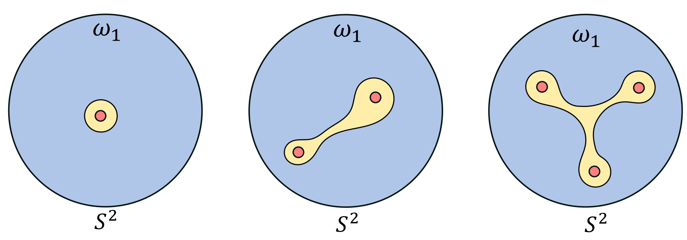
Figure 2: Subsystem choices: (left) to study the bulk; (mid)-(right) to study the gapped boundaries.

II.2 Characterizing bulk anyons

Σ⁡(Ω)\Sigma(\Omega) always contains the reduced density matrix σΩ1≡trΩ¯​|ψ⟩​⟨ψ|\sigma^{1}_{\Omega}\equiv\textrm{tr}_{\bar{\Omega}}|\psi\rangle\langle\psi| of the “global” ground state |ψ⟩|\psi\rangle. For a topologically trivial subsystem ω\omega (e.g. ω1\omega_{1} and ω2\omega_{2} in Fig. 2, we have Σ⁡(ω)={σω1}\Sigma(\omega)=\{\sigma_{\omega}^{1}\}. In other words, states locally minimizing the energy of subsystem ω\omega are indistinguishable from the global ground state on the subsystem. Though simple, Σ⁡(ω)\Sigma(\omega) determines the possible types of deformable strings in Fig. 1 and that the string operators can be unitary (see Sec. IV.3 for details).

On the other hand, the information convex of a bulk annulus Ω1\Omega_{1} has a richer structure:

Σ⁡(Ω1)={σΩ1|σΩ1=∑apa​σΩ1a},\Sigma(\Omega_{1})=\{\sigma_{\Omega_{1}}|\sigma_{\Omega_{1}}=\sum_{a}p_{a}\sigma_{\Omega_{1}}^{a}\}, (1)

where aa labels bulk superselection sectors (bulk anyon types), with a=1a=1 for the vacuum sector. {pa|∑apa=1}\{p_{a}|\sum_{a}p_{a}=1\} is a probability distribution. Clearly, Σ⁡(Ω1)\Sigma(\Omega_{1}) is a convex set and σΩ1a\sigma^{a}_{\Omega_{1}} are its extremal points. Under continuous deformations of Ω1\Omega_{1} and the Hamiltonian, Σ⁡(Ω1)\Sigma({\Omega_{1}}) exhibits the following topological invariant structure:

S⁡(σΩ1a)\displaystyle S(\sigma^{a}_{\Omega_{1}}) =\displaystyle= S⁡(σΩ11)+ln⁡da2\displaystyle S(\sigma^{1}_{\Omega_{1}})+\ln d_{a}^{2} (2)
σΩ1a⋅σΩ1b\displaystyle\sigma^{a}_{\Omega_{1}}\cdot\sigma^{b}_{\Omega_{1}} =\displaystyle= 0for​a≠b;\displaystyle 0\quad\textrm{for}\,\,\,\,a\neq b;\quad (3)
t​r​[σΩ1a⋅σΩ1a]t​r​[σΩ11⋅σΩ11]\displaystyle\frac{tr[\sigma^{a}_{\Omega_{1}}\cdot\sigma^{a}_{\Omega_{1}}]}{tr[\sigma^{1}_{\Omega_{1}}\cdot\sigma^{1}_{\Omega_{1}}]} =\displaystyle= 1da2\displaystyle\frac{1}{d^{2}_{a}} (4)

where S⁡(σ)=−t​r​(σ​ln⁡σ)S(\sigma)=-tr(\sigma\ln\sigma) is the von Neumann entropy. One can further show the extremal point σΩ1a=t​rΩ¯1​|φa⟩​⟨φa|\sigma^{a}_{\Omega_{1}}=tr_{\bar{\Omega}_{1}}|\varphi^{a}\rangle\langle\varphi^{a}| can be obtained from an excited state |φa⟩|\varphi^{a}\rangle with an anyon pair (a,a¯)(a,\bar{a}) created by a bulk string shown in Fig. 3(b). When Ω1\Omega_{1} is a noncontractible annulus on a torus T2T^{2}, each extremal point can be obtained from the corresponding minimal entangled state on torus [17].

In the example of S3S_{3} quantum double, there are 8 extremal points (8 anyons), leading to a 7-dimensional information convex Σ⁡(Ω1)\Sigma(\Omega_{1}).

Refer to caption
Figure 3: (a) A 2D projection of 7D convex set Σ⁡(Ω1)\Sigma(\Omega_{1}) which has 8 extremal points. (b) Preparing an extremal point σΩ1a∈Σ⁡(Ω1)\sigma_{\Omega_{1}}^{a}\in\Sigma(\Omega_{1}) by a bulk process. (c) Divide Ω1\Omega_{1} into A,B,CA,B,C.

II.3 TEE as a saturated lower bound

The information convex Σ⁡(Ω1)\Sigma(\Omega_{1}) naturally encodes the TEE as a saturated lower bound. Let σ~Ω1\tilde{\sigma}_{\Omega_{1}} be the element located at the “center” of Σ⁡(Ω1)\Sigma(\Omega_{1}), written as

σ~Ω1=∑ada2𝒟2​σΩ1a\tilde{\sigma}_{\Omega_{1}}=\sum_{a}\frac{d_{a}^{2}}{\mathcal{D}^{2}}\,\sigma^{a}_{\Omega_{1}} (5)

It has the maximally entanglement entropy among all density matrices in Σ⁡(Ω1)\Sigma(\Omega_{1}). Then, let us take the partition Ω1=A​B​C\Omega_{1}=ABC as is shown in Fig. 3(c) and define TEE St​o​p​o≡(SA​B+SB​C−SB−SA​B​C)|σ1S_{topo}\equiv(S_{AB}+S_{BC}-S_{B}-S_{ABC})|_{\sigma^{1}} in accordance with Levin-Wen [16]. Then one could derive a lower bound St​o​p​o≥S⁡(σ~Ω1)−S⁡(σΩ11)S_{topo}\geq S(\tilde{\sigma}_{\Omega_{1}})-S(\sigma^{1}_{\Omega_{1}}) by noticing the following two facts:

  • •

    The form of St​o​p​oS_{topo} above is the conditional mutual information. It is an important theorem (the strong subadditivity condition) that conditional mutual information is always nonnegative, i.e. (SA​B+SB​C−SB−SA​B​C)|σ≥0(S_{AB}+S_{BC}-S_{B}-S_{ABC})|_{\sigma}\geq 0 for any density matrix σ\sigma.

  • •

    All density matrices in Σ⁡(Ω1)\Sigma(\Omega_{1}) have the same reduced density matrix on A​BAB, B​CBC and BB because Σ⁡(ω1)\Sigma({\omega_{1}}) contains a single element.

Furthermore, it is known that under general assumptions in [30], σ~Ω1\tilde{\sigma}_{\Omega_{1}} saturates the strong subadditivity condition. This allows us to reformulate the celebrated TEE as a saturated lower bound:

St​o​p​o=S⁡(σ~Ω1)−S⁡(σΩ11)=ln⁡𝒟2S_{topo}=S(\tilde{\sigma}_{\Omega_{1}})-S(\sigma^{1}_{\Omega_{1}})=\ln\mathcal{D}^{2} (6)

where 𝒟≡∑ada2\mathcal{D}\equiv\sqrt{\sum_{a}d_{a}^{2}} is the total quantum dimension. See Sec. IV.4 for more details of the derivation and further discussions.

II.4 Characterizing boundary topological excitations

The topological excitations on the gapped boundary can be extracted by choosing subsystem Ω2\Omega_{2} in Fig. 2:

Σ⁡(Ω2)\displaystyle\Sigma(\Omega_{2}) =\displaystyle= {σΩ2|σΩ2=∑αpα​σΩ2α}.\displaystyle\{\sigma_{\Omega_{2}}|\sigma_{\Omega_{2}}=\sum_{\alpha}p_{\alpha}\sigma_{\Omega_{2}}^{\alpha}\}. (7)
S⁡(σΩ2α)\displaystyle S(\sigma^{\alpha}_{\Omega_{2}}) =\displaystyle= S⁡(σΩ21)+ln⁡dα2,\displaystyle S(\sigma^{1}_{\Omega_{2}})+\ln{d_{\alpha}^{2}}, (8)
σΩ2α⋅σΩ2β\displaystyle\sigma^{\alpha}_{\Omega_{2}}\cdot\sigma^{\beta}_{\Omega_{2}} =\displaystyle= 0for​α≠β;\displaystyle 0\quad\textrm{for}\,\,\,\,\alpha\neq\beta;\quad (9)
t​r​[σΩ2α⋅σΩ2α]t​r​[σΩ21⋅σΩ21]\displaystyle\frac{tr[\sigma^{\alpha}_{\Omega_{2}}\cdot\sigma^{\alpha}_{\Omega_{2}}]}{tr[\sigma^{1}_{\Omega_{2}}\cdot\sigma^{1}_{\Omega_{2}}]} =\displaystyle= 1dα2,\displaystyle\frac{1}{d^{2}_{\alpha}}, (10)

where {pα}\{p_{\alpha}\} is a probability distribution. The structure of Σ⁡(Ω2)\Sigma(\Omega_{2}) is very similar to that of Σ⁡(Ω1)\Sigma(\Omega_{1}), except that the α,β\alpha,\beta label the boundary superselection sectors instead of the bulk ones. The name comes from the fact that every extremal point σΩ2α\sigma_{\Omega_{2}}^{\alpha} can be obtained from an excited state with a unitary string operator acting along the boundary, which creates a pair of boundary topological excitations (α,α¯)(\alpha,\bar{\alpha}) as shown in Fig. 4(b).

For a K={1}K=\{1\} boundary of GG quantum double, α∈G\alpha\in G labels the “flux” type and dα=1d_{\alpha}=1, ∀α∈G\forall~\alpha\in G. For G=S3G=S_{3}:

α\alpha  11  rr r2r^{2}  ss  s​rsr  s​r2sr^{2}
dαd_{\alpha} 1 1 1 1 1 1

For a general quantum double model with an untwisted K⊆GK\subseteq G boundary, we use the information convex to identify deconfined topological excitations along the boundary, in contrast to the confined boundary excitations discussed in Ref. [27]. However, our calculations show that they share the same algebraic structure as in [27].

Refer to caption
Figure 4: (a) A 2D projection of 5D convex set Σ⁡(Ω2)\Sigma(\Omega_{2}) for S3S_{3} quantum double, which has 6 extremal points. Σ​(Ω2)b​u​l​k⊆Σ⁡(Ω2)\Sigma(\Omega_{2})_{bulk}\subseteq\Sigma(\Omega_{2}) is a 2D convex set with 3 extremal points. (b) A boundary process that prepares an extremal point σΩ2α∈Σ⁡(Ω2)\sigma^{\alpha}_{\Omega_{2}}\in\Sigma(\Omega_{2}). (c) A bulk process that prepares an extremal point of Σ​(Ω2)b​u​l​k\Sigma(\Omega_{2})_{bulk}. (d) A pair of bulk non-Abelian anyons (a,a¯)(a,\bar{a}) created by a boundary process. (e) A (a¯,α)(\bar{a},\alpha) pair created by a boundary process.

We use Σ⁡(Ω2)\Sigma(\Omega_{2}) to demonstrate the relation between bulk anyons and boundary topological excitations, focusing on non-Abelian topological orders. For quantum double with Abelian group GG and any untwisted K⊆GK\subseteq G boundary, all extremal points of Σ⁡(Ω2)\Sigma(\Omega_{2}) can be obtained by creating a bulk anyon pair (a,a¯)(a,\bar{a}) with a bulk string crossing Ω2\Omega_{2}, see Fig. 4(c). On the other hand, for a non-Abelian GG with a K={1}K=\{1\} boundary, bulk excitations in Fig. 4(c) can only explore a (convex) subset Σ​(Ω2)b​u​l​k⊊Σ⁡(Ω2)\Sigma(\Omega_{2})_{bulk}\subsetneq\Sigma(\Omega_{2}) of the information convex Σ⁡(Ω2)\Sigma(\Omega_{2}).

For G=S3G=S_{3}, K={1}K=\{1\} case, we find:

Σ​(Ω2)b​u​l​k={σΩ2|σΩ2=p1​σΩ21+pcr​σΩ2cr+pcs​σΩ2cs},\Sigma(\Omega_{2})_{bulk}=\{\sigma_{\Omega_{2}}|\sigma_{\Omega_{2}}=p_{1}\sigma^{1}_{\Omega_{2}}+p_{c_{r}}\sigma^{c_{r}}_{\Omega_{2}}+p_{c_{s}}\sigma^{c_{s}}_{\Omega_{2}}\}, (11)

where {p1,pcr,pcs}\{p_{1},p_{c_{r}},p_{c_{s}}\} is a probability distribution, and

σΩ2cr≡12​(σΩ2r+σΩ2r2),σΩ2cs≡13​(σΩ2s+σΩ2s​r+σΩ2s​r2).\sigma^{c_{r}}_{\Omega_{2}}\equiv\frac{1}{2}(\sigma_{\Omega_{2}}^{r}+\sigma_{\Omega_{2}}^{r^{2}}),\quad\sigma^{c_{s}}_{\Omega_{2}}\equiv\frac{1}{3}(\sigma^{s}_{\Omega_{2}}+\sigma^{sr}_{\Omega_{2}}+\sigma^{sr^{2}}_{\Omega_{2}}). (12)

The bulk anyon pair (a,a¯)(a,\bar{a}) associated with extremal points of Σ​(Ω2)b​u​l​k\Sigma(\Omega_{2})_{bulk} is a∈{1,A,Jw}a\in\{1,A,J^{w}\} for σΩ21\sigma_{\Omega_{2}}^{1}, a∈{Jx,Jy,Jz}a\in\{J^{x},J^{y},J^{z}\} for σΩ2cr\sigma_{\Omega_{2}}^{c_{r}}, and a∈{Ka,Kb}a\in\{K^{a},K^{b}\} for σΩ2cs\sigma_{\Omega_{2}}^{c_{s}}. In this case, while boundary topological excitations can lead to all extremal points in Σ⁡(Ω2)\Sigma(\Omega_{2}), only one extremal point σΩ21\sigma_{\Omega_{2}}^{1} can be obtained by anyons connected by a bulk string.

What are the relation and distinction between bulk and boundary topological excitations? First of all, each boundary topological excitation as in Fig. 4(b) can be deformed into the bulk as in Fig. 4(d) by local unitary operators, although the string may not completely detach from the boundary. However, such a bulk pair (a,a¯)(a,\bar{a}) connected by a boundary string in Fig. 4(d) should not be identified with a pair connected by a pure bulk string in Fig. 4(c), since they may correspond to different elements in the information convex.

In G=S3,K={1}G=S_{3},~K=\{1\} quantum double, a boundary excitation pair (α=r,α¯=r2)(\alpha=r,\bar{\alpha}=r^{2}) in Fig. 4(b) can be deformed into a bulk pair (a=Jx,a¯=Jx)(a=J^{x},\bar{a}=J^{x}) connected by a boundary string in Fig. 4(d), and they both lead to the extremal point σΩ2α=σΩ2r\sigma^{\alpha}_{\Omega_{2}}=\sigma^{r}_{\Omega_{2}} in Fig. 4(a). In contrast, a pair of bulk anyons (Jx,Jx)(J^{x},J^{x}) in Fig. 4(c) only gives rise to σΩ2cr\sigma^{c_{r}}_{\Omega_{2}} in Fig. 4(a).

Secondly, each bulk anyon aa in Fig. 4(c), when “moved” to the boundary in Fig. 4(e) by local unitary operators, is generally deformed into a superposition ∑α\sum\alpha of boundary topological excitations. This process is governed by certain condensation rules a→∑αa\rightarrow\sum\alpha [21, 20, 27], which manifests in the information convex.

Specifically in G=S3,K={1}G=S_{3},~K=\{1\} case, Eq. (12) of the information convex Σ⁡(Ω2)\Sigma(\Omega_{2}) corresponds to the anyon condensation rules of K={1}K=\{1\} boundary of G=S3G=S_{3} quantum double, summarized below:

cc c1={1}c_{1}=\{1\} cr={r,r2}c_{r}=\{r,r^{2}\} cs={s,s​r,s​r2}c_{s}=\{s,sr,sr^{2}\}
aa  11  AA JwJ^{w}     JxJ^{x}     JyJ^{y}     JzJ^{z}     KaK^{a}     KbK^{b}
α\alpha  11  11 2⋅12\cdot 1  rr r2r^{2}  rr r2r^{2}  rr r2r^{2}  ss s​rsr s​r2sr^{2}  ss s​rsr s​r2sr^{2}

Here each of the bulk anyons {Jx,Jy,Jz,Ka,Kb}\{J^{x},J^{y},J^{z},K^{a},K^{b}\} becomes a superposition of boundary topological excitations, once moved to the boundary as in Fig. 4(e) by a local unitary operator. For instance, consider a bulk anyon pair (a=Jx,a¯=Jx)(a=J^{x},\bar{a}=J^{x}) in Fig. 4(c). Local unitaries can deform the bulk string and move anyon a=Jxa=J^{x} to the boundary as in Fig. 4(e). However, this bulk anyon a=Jxa=J^{x} cannot turn into a single boundary superselection sector by any local unitary: instead, it “condenses into” a superposition of boundary topological excitations Jx→r+r2J^{x}\rightarrow r+r^{2}, in accordance with Eq. (12).

II.5 Anyon condensation to the boundary

Previously, Σ⁡(Ω2)\Sigma(\Omega_{2}) already demonstrates the anyon condensation on the gapped boundary [21, 22, 27, 31]. Here we discuss a unique consequence of boundary anyon condensation rules of non-Abelian topological orders, where the information convex Σ⁡(Ω3)\Sigma(\Omega_{3}) for subsystem Ω3\Omega_{3} (see Fig. 5) can have an infinite number of extremal points.

Refer to caption
Figure 5: (a) A 3D projection of 5D convex set Σ⁡(Ω3)\Sigma(\Omega_{3}) which has extremal points on a sphere S2S^{2} plus two isolated points. (b) A boundary process that prepares an extremal point of Σ⁡(Ω3)\Sigma(\Omega_{3}), where a=1,A,Jwa=1,A,J^{w}. (c) Braiding an (α,α¯)(\alpha,\bar{\alpha}) pair along the boundary corresponds to a unitary operation W⁡(α)W(\alpha) supported on the yellow loop.

Consider annulus Ω3\Omega_{3} covering the boundary in Fig. 5, for K={1}K=\{1\} gapped boundary of G=S3G=S_{3} quantum double, the information convex Σ⁡(Ω3)\Sigma(\Omega_{3}) has the following extremal points: σΩ31\sigma^{1}_{\Omega_{3}}, σΩ3A\sigma^{A}_{\Omega_{3}}, and σΩ3Jw​(θ,ϕ)\sigma^{J^{w}}_{\Omega_{3}}(\theta,\phi), where (θ,ϕ)(\theta,\phi) parametrize a sphere S2S^{2} as shown in Fig. 5(a),

Σ(Ω3)={σΩ3|σΩ3\displaystyle\Sigma(\Omega_{3})=\{\sigma_{\Omega_{3}}|\sigma_{\Omega_{3}} =\displaystyle= p1​σΩ31+pA​σΩ3A\displaystyle p_{1}\sigma_{\Omega_{3}}^{1}+p_{A}\sigma^{A}_{\Omega_{3}} (13)
+∫dθdϕp(θ,ϕ)σΩ3Jw(θ,ϕ)},\displaystyle+\int d\theta d\phi\,\,p(\theta,\phi)\,\sigma^{J^{w}}_{\Omega_{3}}(\theta,\phi)\},\qquad

with nonnegative p1p_{1}, pAp_{A}, p⁡(θ,ϕ)p(\theta,\phi) satisfying p1+pA+∫d​θ​𝑑ϕ​p​(θ,ϕ)=1p_{1}+p_{A}+\int d\theta d\phi\,p(\theta,\phi)=1. Moreover, Σ⁡(Ω3)\Sigma(\Omega_{3}) has the following structure:

S⁡(σΩ3A)\displaystyle S(\sigma^{A}_{\Omega_{3}}) =\displaystyle= S⁡(σΩ31)+ln⁡dA,\displaystyle S(\sigma^{1}_{\Omega_{3}})+\ln d_{A}, (14)
S⁡(σΩ3Jw​(θ,ϕ))\displaystyle S(\sigma^{J^{w}}_{\Omega_{3}}(\theta,\phi)) =\displaystyle= S⁡(σΩ31)+ln⁡dJw;\displaystyle S(\sigma^{1}_{\Omega_{3}})+\ln d_{J^{w}}; (15)
σΩ31⋅σΩ3A=σΩ31⋅σΩ3Jw​(θ,ϕ)\displaystyle\sigma^{1}_{\Omega_{3}}\cdot\sigma^{A}_{\Omega_{3}}=\sigma^{1}_{\Omega_{3}}\cdot\sigma^{J^{w}}_{\Omega_{3}}(\theta,\phi) =\displaystyle= σΩ3A⋅σΩ3Jw​(θ,ϕ)=0;\displaystyle\sigma^{A}_{\Omega_{3}}\cdot\sigma^{J^{w}}_{\Omega_{3}}(\theta,\phi)=0;\qquad (16)
t​r​[σΩ3A⋅σΩ3A]t​r​[σΩ31⋅σΩ31]\displaystyle\frac{tr[\sigma^{A}_{\Omega_{3}}\cdot\sigma^{A}_{\Omega_{3}}]}{tr[\sigma^{1}_{\Omega_{3}}\cdot\sigma^{1}_{\Omega_{3}}]} =\displaystyle= 1dA;\displaystyle\frac{1}{d_{A}}; (17)
t​r​[σΩ3Jw​(θ,ϕ)⋅σΩ3Jw​(θ′,ϕ′)]t​r​[σΩ31⋅σΩ31]\displaystyle\frac{tr[\sigma^{J^{w}}_{\Omega_{3}}(\theta,\phi)\cdot\sigma^{J^{w}}_{\Omega_{3}}(\theta^{\prime},\phi^{\prime})]}{tr[\sigma^{1}_{\Omega_{3}}\cdot\sigma^{1}_{\Omega_{3}}]} =\displaystyle= 1dJw⋅1+n^⋅n^′2,\displaystyle\frac{1}{d_{J^{w}}}\cdot\frac{1+\hat{n}\cdot\hat{n}^{\prime}}{2}, (18)

where the unit vector n^=(sin⁡θ​cos⁡ϕ,sin⁡θ​sin⁡ϕ,cos⁡θ)\hat{n}=(\sin\theta\cos\phi,\sin\theta\sin\phi,\cos\theta), and similarly for n^′\hat{n}^{\prime} in terms of (θ′,ϕ′)(\theta^{\prime},\phi^{\prime}).

We notice that braiding a (α,α¯)(\alpha,\bar{\alpha}) pair around the boundary before annihilation, implemented by a unitary operator W⁡(α)W(\alpha) supported on the closed loop in Fig. 5(c), do not change the energy density anywhere. Therefore this operation generates a (structure preserving) bijective map σΩ3∈Σ⁡(Ω3)→W⁡(α)​σΩ3​W​(α)†∈Σ⁡(Ω3)\sigma_{\Omega_{3}}\in\Sigma(\Omega_{3})\rightarrow W(\alpha)\sigma_{\Omega_{3}}W({{\alpha}})^{\dagger}\in\Sigma(\Omega_{3}). Explicitly, each W⁡(α)W(\alpha) keeps the extremal points σΩ31\sigma^{1}_{\Omega_{3}} and σΩ3A\sigma^{A}_{\Omega_{3}} fixed but rotates on the sphere of σΩ3Jw​(θ,ϕ)\sigma^{J^{w}}_{\Omega_{3}}(\theta,\phi). The set of rotations are generated by W⁡(r)W(r): (θ,ϕ)→(θ,ϕ+2​π/3)(\theta,\phi)\rightarrow(\theta,\phi+2\pi/3) and W⁡(s)W(s): (θ,ϕ)→(π−θ,−ϕ)(\theta,\phi)\rightarrow(\pi-\theta,-\phi), and they realize the S3S_{3} group action on sphere S2S^{2}.

While σΩ31\sigma^{1}_{\Omega_{3}} is obtained from the ground state, the extremal point σΩ3A\sigma^{A}_{\Omega_{3}} (or σΩ3Jw​(θ,ϕ)\sigma^{J^{w}}_{\Omega_{3}}(\theta,\phi)) is prepared by an excited state with a single anyon AA (or JwJ^{w}) in the bulk, created by a string attached to the boundary as in Fig. 5(b). The (θ,ϕ)(\theta,\phi) dependence for σΩ3Jw\sigma_{\Omega_{3}}^{J^{w}} comes from the condensation multiplicity 22 in Jw→2⋅1J^{w}\to 2\cdot 1. The two ways to condense JwJ^{w} into the boundary lead to a two-dimensional protected Hilbert space, which result in a set of reduced density matrices {σΩ3Jw​(θ,ϕ)}\{\sigma_{\Omega_{3}}^{J^{w}}(\theta,\phi)\} parametrized by (θ,ϕ)∈S2(\theta,\phi)\in S^{2}. Such condensation multiplicity and infinite extremal points are unique to non-Abelian topological orders.

Though σΩ3Jw\sigma^{J^{w}}_{\Omega_{3}} with different (θ,ϕ)(\theta,\phi) share the same entanglement entropy and entanglement spectrum [32], their “interference pattern” in Eq. (18) leaves a clear signature for the infinite extremal points σΩ3Jw​(θ,ϕ)\sigma^{J^{w}}_{\Omega_{3}}(\theta,\phi).

II.6 Potential measurements of information convex structure

It is an interesting question whether the structure of the information convex could be observed experimentally. One challenge is the creation of anyons and another is the measurement of properties directly related to density matrices. Recently, cold atom experiments seem to have made progress in both directions. Anyons are claimed to be created in a minimal toric code Hamiltonian [33] and the corresponding braiding properties are studied. The recent interference experiments [34, 35] allow people to measure t​r​[σΩ(1)⋅σΩ(2)]tr[\sigma_{\Omega}^{(1)}\cdot\sigma_{\Omega}^{(2)}] for any Ω\Omega. In the interference experiment, two identical copies of a cold atom system are created. Then, the authors prepare the two copies of the system in pure state |φ(1)⟩|\varphi^{(1)}\rangle and |φ(2)⟩|\varphi^{(2)}\rangle respectively. The quantum state of the two copies of the system |φ(1)⟩|\varphi^{(1)}\rangle and |φ(2)⟩|\varphi^{(2)}\rangle can be either the same or different and

σΩ(1)=t​rΩ¯​|φ(1)⟩​⟨φ(1)|,σΩ(2)=t​rΩ¯​|φ(2)⟩​⟨φ(2)|\sigma_{\Omega}^{(1)}=tr_{\bar{\Omega}}|\varphi^{(1)}\rangle\langle\varphi^{(1)}|,\quad\sigma_{\Omega}^{(2)}=tr_{\bar{\Omega}}|\varphi^{(2)}\rangle\langle\varphi^{(2)}| (19)

The interference of these two copies of the system allows people to measure t​r​[σΩ(1)⋅σΩ(2)]tr[\sigma_{\Omega}^{(1)}\cdot\sigma_{\Omega}^{(2)}]. It seems possible to observe the structure of information convex in this type of cold atom experiment.

One could cool down the system except for several isolated points such that Ω\Omega, a subsystem being cooled down, contains no excitations. Then the information convex gives prediction for the measurement result of t​r​[σΩ(1)⋅σΩ(2)]tr[\sigma_{\Omega}^{(1)}\cdot\sigma_{\Omega}^{(2)}] for topological orders. For example:

  • •

    First, in the simplest situation, both |φ(1)⟩|\varphi^{(1)}\rangle and |φ(2)⟩|\varphi^{(2)}\rangle are in the ground state. Then, the interference experiment measures t​r​[σΩ1⋅σΩ1]tr[\sigma^{1}_{\Omega}\cdot\sigma^{1}_{\Omega}] for all subsystems Ω\Omega. It is always a positive number, which may be used to normalize the rest of the results.

  • •

    Suppose on the state |φ(1)⟩|\varphi^{(1)}\rangle a pair of bulk anyons (a,a¯)(a,\bar{a}) is created and the state |φ(2)⟩|\varphi^{(2)}\rangle is the ground state. Here a≠1a\neq 1. Then, according to Eq. (3), we get 00 on any annulus surrounding the anyon aa, since t​r​[σΩ11⋅σΩ1a]=0tr[\sigma^{1}_{\Omega_{1}}\cdot\sigma^{a}_{\Omega_{1}}]=0. A similar result holds for any annulus surrounding the anyon a¯\bar{a}.

  • •

    Suppose on the state |φ(1)⟩|\varphi^{(1)}\rangle a pair of boundary topological excitations (α,α¯)(\alpha,\bar{\alpha}) is created and the state |φ(2)⟩|\varphi^{(2)}\rangle is the ground state. Here α≠1\alpha\neq 1. Then, according to Eq. (9), we get 00 on any subsystem of Ω2\Omega_{2} topology surrounding the boundary topological excitation α\alpha, since t​r​[σΩ21⋅σΩ2α]=0tr[\sigma^{1}_{\Omega_{2}}\cdot\sigma^{\alpha}_{\Omega_{2}}]=0. A similar result holds for any subsystem of Ω2\Omega_{2} topology surrounding the boundary topological excitation α¯\bar{\alpha}.

  • •

    Suppose on the state |φ(1)⟩|\varphi^{(1)}\rangle a bulk anyon JwJ^{w} discussed above is created with a condensation channel labeled by (θ,ϕ)(\theta,\phi), and on the state |φ(2)⟩|\varphi^{(2)}\rangle a bulk anyon JwJ^{w} discussed above is created with a condensation channel labeled by (θ′,ϕ′)(\theta^{\prime},\phi^{\prime}). Note that, we do not require the two anyons be created at the same location. Then, according to Eq. (18), for each subsystem of Ω3\Omega_{3} topology, we get an interference result depending on the condensation channel, i.e.

    t​r​[σΩ3Jw​(θ,ϕ)⋅σΩ3Jw​(θ′,ϕ′)]∼1+n^⋅n^′2tr[\sigma^{J^{w}}_{\Omega_{3}}(\theta,\phi)\cdot\sigma^{J^{w}}_{\Omega_{3}}(\theta^{\prime},\phi^{\prime})]\sim\frac{1+\hat{n}\cdot\hat{n}^{\prime}}{2} (20)
  • •

    For a system with multiple gapped boundaries (or closed manifold like a torus) which typically give rise to multiple ground states, we could observe signatures even without excitations.

On the other hand, no features listed above are expected for any short-range entangled phase without topological excitations.

For real experiments, a challenge is to prepare relatively large identical copies of the system. Another challenge is to make accurate interference measurement in large systems. Typically, the number of measurements to make a prediction for t​r​[σΩ(1)⋅σΩ(2)]tr[\sigma_{\Omega}^{(1)}\cdot\sigma_{\Omega}^{(2)}] with a given precision grows very fast as system size grows. Therefore, it would be a difficult experiment. A good news is that a single interference simultaneously measure t​r​[σΩ(1)⋅σΩ(2)]tr[\sigma_{\Omega}^{(1)}\cdot\sigma_{\Omega}^{(2)}] for a lot of different subsystems Ω\Omega. Therefore, it should be possible to obtain a good accuracy of information convex structure with a much fewer number of measurements than what is required to measure the 2nd-Renyi entropy for a single subsystem Ω\Omega. We hope this type of experimental detection of the information convex structure will be possible in the future.

III The Information convex

We provide a definition of information convex Σ⁡(Ω,Ω′)\Sigma(\Omega,\Omega^{\prime}) and Σ⁡(Ω)\Sigma(\Omega) for frustration-free local Hamiltonians and discuss some basic properties. Generalizations beyond frustration-free local Hamiltonians are briefly discussed.

III.1 Frustration-free local Hamiltonians

We use the following definition of frustration-free local Hamiltonians in the context of lattice models. This definition of frustration-free local Hamiltonian is similar to the definition in Ref. [28].

Definition III.1 (Frustration-free local Hamiltonians).

A frustration-free local Hamiltonian is a Hamiltonian written as H=∑ihiH=\sum_{i}h_{i}, which satisfies the following:

1) Each hih_{i} is a Hermitian operator acting on links within a local region of finite size RR. To simplify our notations below, we will assume the minimal eigenvalue of each hih_{i} to be 00.

2) hi​P0=0,∀ih_{i}P_{0}=0,\forall i, where P0P_{0} is the projector onto the subspace of ground states of HH. In other words, every hih_{i} obtains its minimal eigenvalue 00 on a ground state |ψ⟩|\psi\rangle, i.e. hi​|ψ⟩=0,∀ih_{i}|\psi\rangle=0,\,\forall i.

Let HΩ′H_{\Omega^{\prime}} be the Hamiltonian of subsystem Ω′\Omega^{\prime}, i.e. keeping terms of HH which are supported on the subsystem Ω′\Omega^{\prime}. One can easily check that the ground state |ψ⟩|\psi\rangle minimize the Hamiltonian HΩ′H_{\Omega^{\prime}}, i.e. HΩ′⊗1Ω¯′​|ψ⟩=0H_{\Omega^{\prime}}\otimes 1_{\bar{\Omega}^{\prime}}|\psi\rangle=0. Here Ω¯′\bar{\Omega}^{\prime} is the complement of Ω′\Omega^{\prime}.

III.2 The information convex for frustration-free local Hamiltonians

Let us define the information convex for a general frustration-free local Hamiltonian satisfying definition III.1 and study a few basic properties. Note that frustration-free local Hamiltonians include commuting projector Hamiltonians as a subset. Therefore, the definition applies to many exactly solved models of topological orders in 2D, 3D, exactly solved SET models and models related to these exactly solved models by a finite depth quantum circuit.

Definition III.2 (The information convex).

For a frustration-free local Hamiltonian, define the information convex Σ⁡(Ω,Ω′)\Sigma(\Omega,\Omega^{\prime}) to be the set of reduced density matrices on subsystem Ω\Omega obtained from reduced density matrices on a larger subsystem Ω′\Omega^{\prime} (see Fig.6, Ω⊆Ω′⊆S\Omega\subseteq\Omega^{\prime}\subseteq S, SS is the whole system) which minimize the Hamiltonian HΩ′H_{\Omega^{\prime}}, i.e.:

Σ⁡(Ω,Ω′)≡{σΩ|σΩ=t​r[Ω′\Ω]​ρΩ′​where​t​r​[HΩ′​ρΩ′]=0}.\Sigma(\Omega,\Omega^{\prime})\equiv\{\,\sigma_{\Omega}\,|\,\sigma_{\Omega}=tr_{[\Omega^{\prime}\backslash\Omega]}\,\rho_{\Omega^{\prime}}\,\,\,\,\textrm{where}\,\,\,\,tr[H_{\Omega^{\prime}}\rho_{\Omega^{\prime}}]=0\,\}. (21)

For the set to be interesting, we require Ω′\Omega^{\prime} to contain all terms in HH which overlap with Ω\Omega. We use a simpler notation Σ⁡(Ω)\Sigma(\Omega) when we choose the minimal Ω′\Omega^{\prime}.

The definition of Σ⁡(Ω,Ω′)\Sigma(\Omega,\Omega^{\prime}) may be motivated by the consideration that while the set of general reduced density matrices on Ω\Omega has a complicated structure due to the large number of possible excitations, the set of reduced density matrices that minimize the energy around Ω\Omega should have a much simpler structure. Another motivation is that, as we will see, for the quantum double model (which is a zero correlation length commuting projector model) of topological orders, Σ⁡(Ω,Ω′)\Sigma(\Omega,\Omega^{\prime}) and Σ⁡(Ω)\Sigma(\Omega) are small dimensional but nontrivial convex sets depending on subsystem topologies. Homotopically increase Ω′\Omega^{\prime} would not change the set Σ⁡(Ω,Ω′)\Sigma(\Omega,\Omega^{\prime}). Its structure contains important information about the phase. On the other hand, there are frustration-free Hamiltonian models with nonzero correlation length. For these models, the dimension of Σ⁡(Ω)\Sigma(\Omega) may be sensitive to the boundary length and we do not expect Σ⁡(Ω)\Sigma(\Omega) to be stable under an increase of Ω′\Omega^{\prime}. Nevertheless, if the correlation length is finite, we expect Σ⁡(Ω,Ω′)\Sigma(\Omega,\Omega^{\prime}) to (approximately) have a low dimension and simple structure when Ω′\Omega^{\prime} is bigger than Ω\Omega by a few correlation lengths. In this case, it seems better to consider Σ⁡(Ω,Ω′)\Sigma(\Omega,\Omega^{\prime}) instead of Σ⁡(Ω)\Sigma(\Omega).

In the present paper, we do not have to worry about this issue since the calculation is done in a zero correlation length commuting projector model. Nevertheless, some useful properties can be proved with the assumption of frustration-free and we will consider this general class of Hamiltonians in the next section.

Refer to caption
Figure 6: An illustration of subsystem Ω\Omega and Ω′\Omega^{\prime}. Here Ω⊆Ω′\Omega\subseteq\Omega^{\prime}.

III.3 Some general properties

This section contains a few general properties of the information convex Σ⁡(Ω,Ω′)\Sigma(\Omega,\Omega^{\prime}). Most importantly, it is shown that Σ⁡(Ω,Ω′)\Sigma(\Omega,\Omega^{\prime}) is always a compact convex set. This allows us to borrow tools from convex analysis and explore the structure of the convex set Σ⁡(Ω,Ω′)\Sigma(\Omega,\Omega^{\prime}) in this new context. The concept extremal points is introduced. Additional discussions concern some general properties of Σ⁡(Ω,Ω′)\Sigma(\Omega,\Omega^{\prime}) under a change of Ω\Omega or Ω′\Omega^{\prime}.

Theorem III.1.

Σ⁡(Ω,Ω′)\Sigma(\Omega,\Omega^{\prime}) is a convex set.

Here, the set Σ⁡(Ω,Ω′)\Sigma(\Omega,\Omega^{\prime}) being a convex set means the condition that for any two reduced density matrices σΩ(1),σΩ(2)∈Σ⁡(Ω,Ω′)\sigma^{(1)}_{\Omega},\sigma^{(2)}_{\Omega}\in\Sigma(\Omega,\Omega^{\prime}) and arbitrary p∈[0,1]p\in[0,1], we always have p​σΩ(1)+(1−p)​σΩ(2)∈Σ⁡(Ω,Ω′)p\,\sigma^{(1)}_{\Omega}+(1-p)\sigma^{(2)}_{\Omega}\in\Sigma(\Omega,\Omega^{\prime}).

Proof.

For σΩ(1),σΩ(2)∈Σ⁡(Ω,Ω′)\sigma^{(1)}_{\Omega},\sigma^{(2)}_{\Omega}\in\Sigma(\Omega,\Omega^{\prime}), by definition, there exist ρΩ′(1)\rho^{(1)}_{\Omega^{\prime}} and ρΩ′(2)\rho^{(2)}_{\Omega^{\prime}} such that:

σΩ(1)=t​r[Ω′\Ω]​ρΩ′(1),σΩ(2)=t​r[Ω′\Ω]​ρΩ′(2),t​r​[ρΩ′(1)​HΩ′]=t​r​[ρΩ′(2)​HΩ′]=0.\sigma^{(1)}_{\Omega}=tr_{[\Omega^{\prime}\backslash\Omega]}\rho^{(1)}_{\Omega^{\prime}},\quad\sigma^{(2)}_{\Omega}=tr_{[\Omega^{\prime}\backslash\Omega]}\rho^{(2)}_{\Omega^{\prime}},\quad tr[\rho^{(1)}_{\Omega^{\prime}}H_{\Omega^{\prime}}]=tr[\rho^{(2)}_{\Omega^{\prime}}H_{\Omega^{\prime}}]=0. (22)

Therefore, p​ρΩ′(1)+(1−p)​ρΩ′(2)p\rho^{(1)}_{\Omega^{\prime}}+(1-p)\rho^{(2)}_{\Omega^{\prime}} with p∈[0,1]p\in[0,1] is also a density matrix that minimize the Hamiltonian HΩ′H_{\Omega^{\prime}}, and:

p​σΩ(1)+(1−p)​σΩ(2)=t​r[Ω′\Ω]​[p​ρΩ′(1)+(1−p)​ρΩ′(2)]⇒p​σΩ(1)+(1−p)​σΩ(2)∈Σ⁡(Ω,Ω′).p\sigma^{(1)}_{\Omega}+(1-p)\sigma^{(2)}_{\Omega}=tr_{[\Omega^{\prime}\backslash\Omega]}[p\rho^{(1)}_{\Omega^{\prime}}+(1-p)\rho^{(2)}_{\Omega^{\prime}}]\quad\Rightarrow\quad p\sigma^{(1)}_{\Omega}+(1-p)\sigma^{(2)}_{\Omega}\in\Sigma(\Omega,\Omega^{\prime}). (23)

∎

Theorem III.2.

Σ⁡(Ω,Ω′)\Sigma(\Omega,\Omega^{\prime}) is a compact subset of RNR^{{N}}. Here N{N} is a finite number which could depend on the choice of Ω\Omega and Ω′\Omega^{\prime}.

Proof.

The set of all reduced density matrices on Ω\Omega is a compact (closed and bounded) subset of RM2R^{{M}^{2}}. Here M=dimℋ⁡(Ω){M}=\dim\mathcal{H}(\Omega) is the dimension of the Hilbert space on subsystem Ω\Omega. MM is finite for a lattice model with Ω\Omega containing a finite number of links (or sites) and each link (or site) has a corresponding finite-dimensional Hilbert space. Σ⁡(Ω,Ω′)\Sigma(\Omega,\Omega^{\prime}) is a subset of the set of all reduced density matrices on Ω\Omega and therefore it is a bounded subset of RM2R^{{M}^{2}}. Furthermore, Σ⁡(Ω,Ω′)\Sigma(\Omega,\Omega^{\prime}) is closed. Therefore, Σ⁡(Ω,Ω′)\Sigma(\Omega,\Omega^{\prime}) is a compact subset of RNR^{{N}} with finite NN. ∎

Remark.

Theorem III.1 and Theorem III.2 show that Σ⁡(Ω,Ω′)\Sigma(\Omega,\Omega^{\prime}) is a compact convex subset of RNR^{N} for some finite NN. This applies to all the convex sets we will discuss in this paper. We will call them convex sets for short and it is understood that they are compact convex subsets of RNR^{N} for some finite NN.

Definition III.3 (Extremal point).

An extremal point of Σ⁡(Ω,Ω′)\Sigma(\Omega,\Omega^{\prime}) is a reduced density matrix σΩ∈Σ⁡(Ω,Ω′)\sigma_{\Omega}\in\Sigma(\Omega,\Omega^{\prime}) such that if σΩ=p​σΩ(1)+(1−p)​σΩ(2)\sigma_{\Omega}=p\,\sigma^{(1)}_{\Omega}+(1-p)\sigma^{(2)}_{\Omega} with σΩ(1),σΩ(2)∈Σ⁡(Ω,Ω′)\sigma^{(1)}_{\Omega},\sigma^{(2)}_{\Omega}\in\Sigma(\Omega,\Omega^{\prime}) and p∈(0,1)p\in(0,1), then σΩ(1)=σΩ(2)=σΩ\sigma^{(1)}_{\Omega}=\sigma^{(2)}_{\Omega}=\sigma_{\Omega}.

In other words, an extremal point is a point (reduced density matrix) in Σ⁡(Ω,Ω′)\Sigma(\Omega,\Omega^{\prime}) which could not be prepared by other points in Σ⁡(Ω,Ω′)\Sigma(\Omega,\Omega^{\prime}) with a probability distribution.

Proposition III.3.

Σ⁡(Ω,Ω′)\Sigma(\Omega,\Omega^{\prime}) is uniquely determined by the set of extremal points. Furthermore, if Σ⁡(Ω,Ω′)\Sigma(\Omega,\Omega^{\prime}) is nn-dimensional, then any point in Σ⁡(Ω,Ω′)\Sigma(\Omega,\Omega^{\prime}) can be written as a convex combination of at most n+1n+1 extremal points.

Here, convex combination is a combination with a probability distribution {pi}i=1n+1\{p_{i}\}_{i=1}^{n+1}. In other words, for any σΩ∈Σ⁡(Ω,Ω′)\sigma_{\Omega}\in\Sigma(\Omega,\Omega^{\prime}) it is possible to find a (sub)set of extremal points {σΩi}i=1n+1\{\sigma^{i}_{\Omega}\}_{i=1}^{n+1} and a probability distribution {pi}i=1n+1\{p_{i}\}_{i=1}^{n+1} such that σΩ=∑i=1n+1pi​σΩi\sigma_{\Omega}=\sum_{i=1}^{n+1}p_{i}\sigma^{i}_{\Omega}.

Proof.

First, notice that Σ⁡(Ω,Ω′)\Sigma(\Omega,\Omega^{\prime}) is a compact convex subset of RNR^{N} for some finite NN, i.e., the result of theorems III.1 and III.2. Then, use the Minkowski-Caratheodory theorem, 11 1 The Minkowski-Caratheodory theorem together with its generalization to infinite dimension, i.e., the Krein-Milman theorem can be found in the following link: http://math.caltech.edu/Simon_Chp8.pdf., which says that, for Σ\Sigma, a compact convex subset of dimension nn (nn is finite and Σ\Sigma is a subset of RNR^{N} for some finite NN), any point in Σ\Sigma can be written as a convex combination of at most n+1n+1 extremal points. ∎

Proposition III.4.

Every extremal point of Σ⁡(Ω,Ω′)\Sigma(\Omega,\Omega^{\prime}) has a purification in Ω′\Omega^{\prime}. In other words, there exists a pure state |φ⟩Ω′|\varphi\rangle_{\Omega^{\prime}} such that σΩ=t​r[Ω′\Ω]​|φ⟩Ω′​Ω′​⟨φ|\sigma_{\Omega}=tr_{[\Omega^{\prime}\backslash\Omega]}|\varphi\rangle_{\Omega^{\prime}\,\Omega^{\prime}}\langle\varphi|, if σΩ\sigma_{\Omega} is an extremal point of Σ⁡(Ω,Ω′)\Sigma(\Omega,\Omega^{\prime}).

In the following, we discuss a few properties of Σ⁡(Ω,Ω′)\Sigma(\Omega,\Omega^{\prime}) when one tries to change Ω\Omega or Ω′\Omega^{\prime}.

Theorem III.5.

One obtains a convex subset of Σ⁡(Ω,Ω′)\Sigma(\Omega,\Omega^{\prime}) when one replaces Ω′\Omega^{\prime} by a larger subsystem Ω′′\Omega^{\prime\prime}, i.e.:

Σ⁡(Ω,Ω′′)⊆Σ⁡(Ω,Ω′)forΩ′⊆Ω′′.\Sigma(\Omega,\Omega^{\prime\prime})\subseteq\Sigma(\Omega,\Omega^{\prime})\quad\textrm{for}\quad\Omega^{\prime}\subseteq\Omega^{\prime\prime}. (24)
Corollary III.5.1.

Let |ψ⟩|\psi\rangle be a ground state of the frustration-free local Hamiltonian HH. Then, the corresponding reduced density matrix σΩ1≡t​rΩ¯​|ψ⟩​⟨ψ|\sigma_{\Omega}^{1}\equiv tr_{\bar{\Omega}}|\psi\rangle\langle\psi| satisfies σΩ1∈Σ⁡(Ω,Ω′)\sigma_{\Omega}^{1}\in\Sigma(\Omega,\Omega^{\prime}).

Theorem III.6.

The mapping Γ:Σ⁡(Ω,Ω′)→Σ⁡(ω,Ω′)\Gamma:\Sigma(\Omega,\Omega^{\prime})\rightarrow\Sigma(\omega,\Omega^{\prime}) defined by Γ⁡[σΩ]=t​r[Ω\ω]​σΩ\Gamma[\sigma_{\Omega}]=tr_{[\Omega\backslash\omega]}\sigma_{\Omega} is surjective and it preserves the convex structure. Here, ω⊆Ω\omega\subseteq\Omega.

Proof.

The mapping Γ\Gamma is surjective. This follows from t​r[Ω′\ω]=t​r[Ω\ω]​t​r[Ω′\Ω]tr_{[\Omega^{\prime}\backslash\omega]}=tr_{[\Omega\backslash\omega]}tr_{[\Omega^{\prime}\backslash\Omega]}. The following is about the convex structure. Let σΩ(1),σΩ(2)∈Σ⁡(Ω,Ω′)\sigma^{(1)}_{\Omega},\sigma^{(2)}_{\Omega}\in\Sigma(\Omega,\Omega^{\prime}), and p∈[0,1]p\in[0,1]. From the linearity of the t​r[Ω\ω]tr_{[\Omega\backslash\omega]} operation, we have:

Γ⁡[p​σΩ(1)+(1−p)​σΩ(2)]=p​Γ​[σΩ(1)]+(1−p)​Γ​[σΩ(2)].\Gamma[p\,\sigma^{(1)}_{\Omega}+(1-p)\sigma^{(2)}_{\Omega}]=p\,\Gamma[\sigma^{(1)}_{\Omega}]+(1-p)\Gamma[\sigma^{(2)}_{\Omega}]. (25)

This result shows (by definition) that the mapping Γ\Gamma preserves the convex structure. ∎

Theorem III.6 gives constraints to the number of extremal points.

Corollary III.6.1.

If the number of extremal points of Σ⁡(Ω,Ω′)\Sigma(\Omega,\Omega^{\prime}) is a finite number NΩN_{\Omega}, then the number of extremal points of Σ⁡(ω,Ω′)\Sigma(\omega,\Omega^{\prime}) is a finite number NωN_{\omega} satisfying Nω≤NΩN_{\omega}\leq N_{\Omega}. Furthermore, an extremal point of Σ⁡(ω,Ω′)\Sigma(\omega,\Omega^{\prime}) must be the image of some extremal point of Σ⁡(Ω,Ω′)\Sigma(\Omega,\Omega^{\prime}) under the mapping Γ\Gamma. Here, ω⊆Ω\omega\subseteq\Omega.

Proof.

This result follows from the fact that the image of a nonextremal point of Σ⁡(Ω,Ω′)\Sigma(\Omega,\Omega^{\prime}) cannot be an extremal point of Σ⁡(ω,Ω′)\Sigma(\omega,\Omega^{\prime}) unless it is also the image of an extremal point of Σ⁡(Ω,Ω′)\Sigma(\Omega,\Omega^{\prime}). ∎

Remark.

Constraints for the case with an infinite number of extremal points may also be deduced from theorem III.6.

III.4 Beyond frustration-free local Hamiltonians

In this section, we briefly discuss what we expect for generalizations of information convex to models beyond frustration-free local Hamiltonians and hope that more rigorous results will be available in the future.

Let us first consider a frustration-free local Hamiltonian HH with HΩ′H_{\Omega^{\prime}} having a finite energy gap Δ\Delta (between the ground states and the 1st excited state) and consider a generalization of Σ⁡(Ω,Ω′)\Sigma(\Omega,\Omega^{\prime}) into Σ⁡(Ω,Ω′|ϵ)\Sigma(\Omega,\Omega^{\prime}|\epsilon). Here, 0≤ϵ≪Δ0\leq\epsilon\ll\Delta,

Σ⁡(Ω,Ω′|ϵ)≡{σΩ​(ϵ)|σΩ​(ϵ)=t​r[Ω′\Ω]​ρΩ′​where​t​r​[HΩ′​ρΩ′]∈[0,ϵ]}.\Sigma(\Omega,\Omega^{\prime}|\epsilon)\equiv\{\,\sigma_{\Omega}(\epsilon)\,|\,\sigma_{\Omega}(\epsilon)=tr_{[\Omega^{\prime}\backslash\Omega]}\,\rho_{\Omega^{\prime}}\,\,\,\,\textrm{where}\,\,\,\,tr[H_{\Omega^{\prime}}\rho_{\Omega^{\prime}}]\in[0,\epsilon]\,\}. (26)

It is straightforward to show that Σ⁡(Ω,Ω′|ϵ)\Sigma(\Omega,\Omega^{\prime}|\epsilon) is a convex set. Comparing with Eq. (21), if ϵ>0\epsilon>0, then ρΩ′\rho_{\Omega^{\prime}} can have small mixture of excited states. Due to the large number of excited states, the convex set Σ⁡(Ω,Ω′|ϵ)\Sigma(\Omega,\Omega^{\prime}|\epsilon) with ϵ>0\epsilon>0 will be of a large dimension even if Σ⁡(Ω,Ω′)\Sigma(\Omega,\Omega^{\prime}) is a small dimensional convex set. Nevertheless, Σ⁡(Ω,Ω′|ϵ)\Sigma(\Omega,\Omega^{\prime}|\epsilon) stretches out in the directions of excited states by a “distance” suppressed by ϵ/Δ\epsilon/\Delta. Here, the distance could be measured by the minimal deviation of the fidelity (between σΩ​(ϵ)∈Σ⁡(Ω,Ω′|ϵ)\sigma_{\Omega}(\epsilon)\in\Sigma(\Omega,\Omega^{\prime}|\epsilon) and σΩ∈Σ⁡(Ω,Ω′)\sigma_{\Omega}\in\Sigma(\Omega,\Omega^{\prime})) from 1:

l⁡(σΩ​(ϵ))≡[1−F⁡(σΩ​(ϵ),σΩ)]min,withσΩ​(ϵ)∈Σ⁡(Ω,Ω′|ϵ)andσΩ∈Σ⁡(Ω,Ω′).l(\sigma_{\Omega}(\epsilon))\equiv[1-F(\sigma_{\Omega}(\epsilon),\sigma_{\Omega})]_{\min},\qquad\qquad\textrm{with}\qquad\sigma_{\Omega}(\epsilon)\in\Sigma(\Omega,\Omega^{\prime}|\epsilon)\quad\textrm{and}\quad\sigma_{\Omega}\in\Sigma(\Omega,\Omega^{\prime}). (27)

Here fidelity is defined as F⁡(ρ,σ)≡(t​r​ρ12​σ​ρ12)2F(\rho,\sigma)\equiv\bigg(tr\sqrt{\rho^{\frac{1}{2}}\sigma\rho^{\frac{1}{2}}}\bigg)^{2}. One can show that:

l⁡(σΩ​(ϵ))≤ϵΔfor∀σΩ​(ϵ)∈Σ⁡(Ω,Ω′|ϵ).l(\sigma_{\Omega}(\epsilon))\leq\frac{\epsilon}{\Delta}\quad\qquad\quad\quad\textrm{for}\quad\forall\sigma_{\Omega}(\epsilon)\in\Sigma(\Omega,\Omega^{\prime}|\epsilon). (28)

For 0≤ϵ≪Δ0\leq\epsilon\ll\Delta, we could still approximately treat the convex set Σ⁡(Ω,Ω′|ϵ)\Sigma(\Omega,\Omega^{\prime}|\epsilon) as small dimensional with the same structures as Σ⁡(Ω,Ω′)\Sigma(\Omega,\Omega^{\prime}).

Now let us consider the case beyond frustration-free local Hamiltonians. We focus on the case that local perturbations are added to a gapped frustration-free local Hamiltonian (with energy gap Δ\Delta), the case discussed in [36, 28]. Note that we do need to generalize Σ⁡(Ω,Ω′)\Sigma(\Omega,\Omega^{\prime}) into Σ⁡(Ω,Ω′|ϵ)\Sigma(\Omega,\Omega^{\prime}|\epsilon) with some 0≤ϵ≪Δ0\leq\epsilon\ll\Delta in order to get meaningful structures. Consider a model with topological order and the system is defined on a torus S=T2S=T^{2} with length LL and a correlation length ξ≪L\xi\ll L. For the unperturbed model, the ground state degeneracy is exact and Σ⁡(S,S)\Sigma(S,S) is a convex set with (an infinite number of) extremal points in one to one correspondence with the (pure) ground states. However, local perturbations will split the ground-state energies by the order Δexp(−L/ξ)\Delta\exp(-L/\xi); for a more rigorous bound of the energy splitting see [36, 28]. Therefore, in order to construct a convex set with similar structure as the Σ⁡(S,S)\Sigma(S,S) of the unperturbed model, Σ⁡(S,S)\Sigma(S,S) is no longer a good choice, since it does not keep all the low energy states corresponding to the degenerate ground states of the unperturbed model. We need to choose Σ⁡(S,S|ϵ)\Sigma(S,S|\epsilon) with ϵ∼Δexp(−L/ξ)\epsilon\sim\Delta\exp(-L/\xi) for the perturbed theory.

More generally, we expect the Σ⁡(Ω,Ω′)\Sigma(\Omega,\Omega^{\prime}) for the unperturbed model, with Ω′\Omega^{\prime} thicker than Ω\Omega by length L′≫ξL^{\prime}\gg\xi to be generalized into Σ⁡(Ω,Ω′|ϵ)\Sigma(\Omega,\Omega^{\prime}|\epsilon) with ϵ∼Δexp(−L′/ξ)\epsilon\sim\Delta\exp(-L^{\prime}/\xi). Since exp(−L′/ξ)≪1\exp(-L^{\prime}/\xi)\ll 1, the convex set Σ⁡(Ω,Ω′|ϵ)\Sigma(\Omega,\Omega^{\prime}|\epsilon) is approximately small dimensional and it should have very similar structure to the Σ⁡(Ω,Ω′)\Sigma(\Omega,\Omega^{\prime}) in the unperturbed model.

IV GG quantum double with K⊆GK\subseteq G boundary

IV.1 The Hamiltonian of GG quantum double with K⊆GK\subseteq G boundary

Refer to caption
Figure 7: A square lattice with a boundary, generalization to other lattices is straightforward. Labels are as follows: bulk link ee, boundary link e′e^{\prime}, bulk vertex vv, boundary vertex v′v^{\prime}, and face ff. Note that in our model, e′e^{\prime}, v′v^{\prime} only lie in the 1D boundary lattice shown in thicker line.

A quantum double model on an orientable 2D lattice without boundary is defined for any finite group GG [7, 13]. Let us consider a square lattice shown in Fig. 7, generalization to other lattices is straightforward. On a lattice with a boundary, a gapped boundary can be defined for each subgroup K⊆GK\subseteq G [20, 27]. In addition to the subgroup KK, the boundary can depend on a 2-cocycle of KK [20]. In the current work, we focus on the untwisted boundaries, i.e. those with trivial 2-cocycles.

The total Hilbert space is a tensor product of the Hilbert space on each link. The Hilbert space for each bulk link (labeled by ee) is |G||G| dimensional: ℋe=s​p​a​n​{|g⟩e|g∈G}\mathcal{H}_{e}=span\{\,|g\rangle_{e}\,|\,g\in G\,\}, where {|g⟩e|g∈G}\{\,|g\rangle_{e}\,|\,g\in G\,\} is an orthonormal basis. The Hilbert space for each boundary link (labeled by e′e^{\prime}, thicker links in Fig. 7) is |K||K| dimensional: ℋe′=s​p​a​n​{|k⟩e′|k∈K}\mathcal{H}_{e^{\prime}}=span\{\,|k\rangle_{e^{\prime}}\,|\,k\in K\,\}, where {|k⟩e′|k∈K}\{\,|k\rangle_{e^{\prime}}\,|\,k\in K\,\} is an orthonormal basis. We denote a vertex in the bulk (bulk vertex) as vv and a vertex on the boundary (boundary vertex) as v′v^{\prime}, and denote a face as ff. A bulk site s=(v,f)s=(v,f) is a pair containing a face ff and an adjacent bulk vertex vv, a boundary site s′=(v′,f)s^{\prime}=(v^{\prime},f) is a pair containing a face ff, and an adjacent boundary vertex v′v^{\prime}. Our Hamiltonian for GG quantum double with a K⊆GK\subseteq G boundary is

H=∑v(1−Av)+∑f(1−Bf)+∑v′(1−Av′K).H=\sum_{v}(1-A_{v})+\sum_{f}(1-B_{f})+\sum_{v^{\prime}}(1-A_{v^{\prime}}^{K}). (29)

Constants are added into the Hamiltonian simply to keep the minimal eigenvalue to be zero. Here

Av≡1|G|​∑g∈GAvg;Bf≡Bs1;Av′K≡1|K|​∑k∈KAv′k.A_{v}\equiv\frac{1}{|G|}\sum_{g\in G}A_{v}^{g};\qquad B_{f}\equiv B_{s}^{1};\qquad A_{v^{\prime}}^{K}\equiv\frac{1}{|K|}\sum_{k\in K}A_{v^{\prime}}^{k}. (30)

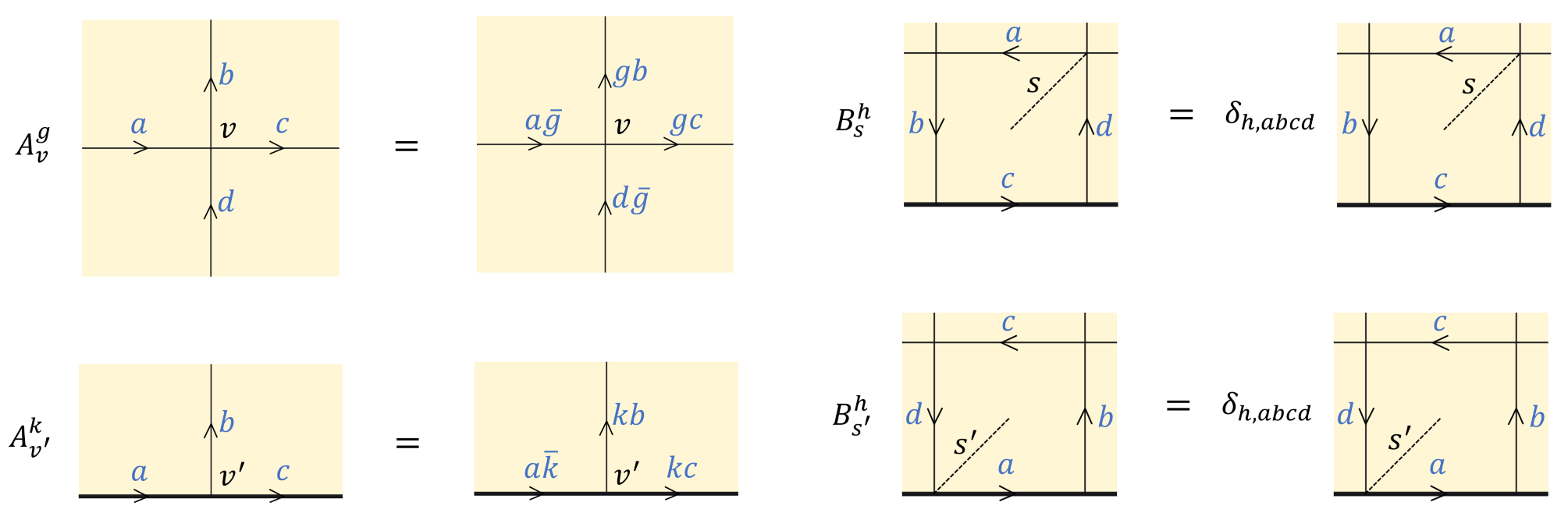
Each operator AvgA_{v}^{g}, BshB_{s}^{h}, Av′kA_{v^{\prime}}^{k}, Bs′hB_{s^{\prime}}^{h} with g,h∈Gg,h\in G and k∈Kk\in K acts on a few links around a vertex or a face. They are defined in Fig. 8.
Refer to caption
Figure 8: The diagram shows the definitions of the operators AvgA_{v}^{g}, BshB_{s}^{h}, Av′kA_{v^{\prime}}^{k}, Bs′hB_{s^{\prime}}^{h} with g,h∈Gg,h\in G and k∈Kk\in K.

One can easily check that all terms in the Hamiltonian commute, and that Av,Bf,Av′KA_{v},B_{f},A_{v^{\prime}}^{K} are projectors (so do 1−Av1-A_{v}, 1−Bf1-B_{f}, 1−Av′K1-A_{v^{\prime}}^{K}), i.e. Av2=AvA_{v}^{2}=A_{v}, Bf2=BfB_{f}^{2}=B_{f}, (Av′K)2=Av′K(A_{v^{\prime}}^{K})^{2}=A_{v^{\prime}}^{K}. A state |ψ⟩|\psi\rangle is a ground state if and only if it satisfies

Av​|ψ⟩=Bf​|ψ⟩=Av′K​|ψ⟩=|ψ⟩,∀v,f,v′.A_{v}|\psi\rangle=B_{f}|\psi\rangle=A_{v^{\prime}}^{K}|\psi\rangle=|\psi\rangle,\qquad\forall\,v,f,v^{\prime}. (31)

For a system with D2D^{2} topology (i.e. cover a disk D2D^{2} with lattice), it can be shown that there is a unique ground state |ψ⟩|\psi\rangle that can be written as (up to normalization)

|ψ⟩=∏vAv⋅∏v′Av′K|1,1,⋯,1⟩.|\psi\rangle=\prod_{v}A_{v}\cdot\prod_{v^{\prime}}A_{v^{\prime}}^{K}|1,1,\cdots,1\rangle. (32)

Here, 11 represents the identity of group GG (or KK). This ground state is an equal weight superposition of all “zero flux” configurations. Let us define the reduced density matrix on subsystem Ω\Omega calculated from the unique ground state |ψ⟩|\psi\rangle as σΩ1\sigma^{1}_{\Omega}, i.e. σΩ1≡t​rΩ¯​|ψ⟩​⟨ψ|\sigma^{1}_{\Omega}\equiv tr_{\bar{\Omega}}|\psi\rangle\langle\psi|, where Ω¯\bar{\Omega} is the complement of Ω\Omega. It will appear many times in later sections.

Remark.

Our Hilbert space and Hamiltonian is closely related to the ones in previous works [20, 27], but there are differences. Our Hilbert space is “smaller” than that in Refs. [20] and [27]. It is the effective Hilbert space when certain terms in the Hamiltonian [20, 27] are not excited. Our Hamiltonian is the effective Hamiltonian of the models in [20, 27] when no excitations of the types discussed above are present. The excitations that could be created in our model also appear in the models in [20, 27], but some of the excitations that could be created in Refs. [20] or [27] may not be created in our model. Especially, the confined excitations inside a boundary [27] do not exist in our model. On the other hand, as will be described below, our model allows a set of deconfined topological excitations to carry boundary superselection sectors α\alpha and quantum dimension dαd_{\alpha}. The set of (α,dα)(\alpha,d_{\alpha}) is coincident with what has been discussed in Ref. [27] for confined boundary excitations. See Eq. (58) and Secs. IV.3,IV.6,IV.8 for more details.

IV.2 The calculation of the information convex for GG quantum double with K⊆GK\subseteq G boundary

The GG quantum double with K⊆GK\subseteq G boundary is a model with commuting projector Hamiltonian Eq. (29), and on a ground state, each projector obtains its minimal eigenvalue 00. Therefore, it is an example of frustration-free local Hamiltonian. The information convex Σ⁡(Ω,Ω′)\Sigma({\Omega,\Omega^{\prime}}) is a convex set uniquely determined by the set of extremal points, see Theorem III.3. Therefore our task here is to find the set of extremal points.

Consider a reduced density matrix ρΩ′\rho_{\Omega^{\prime}} that minimizes the Hamiltonian HΩ′H_{\Omega^{\prime}}. Let us write ρΩ′\rho_{\Omega^{\prime}} in its diagonal form, ρΩ′=∑αλα​|α⟩Ω′​Ω′​⟨α|\rho_{\Omega^{\prime}}=\sum_{\alpha}\lambda_{\alpha}|\alpha\rangle_{\Omega^{\prime}\,\Omega^{\prime}}\langle\alpha| with ⟨α|β⟩Ω′Ω′=δα,β{}_{\Omega^{\prime}}\langle\alpha|\beta\rangle_{\Omega^{\prime}}=\delta_{\alpha,\beta}.

tr(HΩ′ρΩ′)=0⇔HΩ′|α⟩Ω′=0∀α.tr(H_{\Omega^{\prime}}\rho_{\Omega^{\prime}})=0\quad\Leftrightarrow\quad H_{\Omega^{\prime}}|\alpha\rangle_{\Omega^{\prime}}=0\quad\forall\alpha. (33)

In other words, each |α⟩Ω′|\alpha\rangle_{\Omega^{\prime}} is a ground state of HΩ′H_{\Omega^{\prime}}. According to proposition III.4, to find the extremal points of Σ⁡(Ω,Ω′)\Sigma(\Omega,\Omega^{\prime}), it is enough to consider the set of reduced density matrices σΩ=t​r[Ω′\Ω]​|α⟩Ω′​Ω′​⟨α|\sigma_{\Omega}=tr_{[\Omega^{\prime}\backslash\Omega]}|\alpha\rangle_{\Omega^{\prime}\,\Omega^{\prime}}\langle\alpha|.

Let us take the minimal Ω′\Omega^{\prime}, i.e. consider Σ⁡(Ω)\Sigma(\Omega). In this case, HΩ′​|α⟩Ω′=0H_{\Omega^{\prime}}|\alpha\rangle_{\Omega^{\prime}}=0 is equivalent to the following conditions:
(a) Bf​|α⟩Ω′=|α⟩Ω′B_{f}|\alpha\rangle_{\Omega^{\prime}}=|\alpha\rangle_{\Omega^{\prime}}, for f∈∂Ωf\in\partial\Omega.
(b) Bf​|α⟩Ω′=|α⟩Ω′B_{f}|\alpha\rangle_{\Omega^{\prime}}=|\alpha\rangle_{\Omega^{\prime}}, for f∈Ωf\in\Omega.
(c) Avg​|α⟩Ω′=|α⟩Ω′A_{v}^{g}|\alpha\rangle_{\Omega^{\prime}}=|\alpha\rangle_{\Omega^{\prime}} and Av′k​|α⟩Ω′=|α⟩Ω′A_{v^{\prime}}^{k}|\alpha\rangle_{\Omega^{\prime}}=|\alpha\rangle_{\Omega^{\prime}}, for v,v′∈Ωv,v^{\prime}\in\Omega and g∈Gg\in G, k∈Kk\in K.
(d) Avg​|α⟩Ω′=|α⟩Ω′A_{v}^{g}|\alpha\rangle_{\Omega^{\prime}}=|\alpha\rangle_{\Omega^{\prime}} and Av′k​|α⟩Ω′=|α⟩Ω′A_{v^{\prime}}^{k}|\alpha\rangle_{\Omega^{\prime}}=|\alpha\rangle_{\Omega^{\prime}}, for v,v′∈∂Ωv,v^{\prime}\in\partial\Omega and g∈Gg\in G, k∈Kk\in K.
Here, we say f∈Ωf\in\Omega if BfB_{f} is supported on Ω\Omega; we say f∈∂Ωf\in\partial\Omega if BfB_{f} has support overlap with Ω\Omega but is not supported on Ω\Omega; we say v,v′∈Ωv,v^{\prime}\in\Omega if AvgA_{v}^{g} and Av′kA_{v^{\prime}}^{k} are supported on Ω\Omega; we say v,v′∈∂Ωv,v^{\prime}\in\partial\Omega if AvgA_{v}^{g} and Av′kA_{v^{\prime}}^{k} have support overlap with Ω\Omega but not supported on Ω\Omega.

Then, one can show it is possible to write |α⟩Ω′|\alpha\rangle_{\Omega^{\prime}} in the following Schmidt basis:

|α⟩Ω′=∑{haI},λp{haI}λ|{haI};λ⟩Ω⊗|{haI};λ⟩Ω′\Ω⇒σΩ=∑{haI},λp{haI}λ|{haI};λ⟩Ω​Ω⟨{haI};λ|.|\alpha\rangle_{\Omega^{\prime}}=\sum_{\{h^{I}_{a}\},\lambda}\,\sqrt{p^{\lambda}_{\{h^{I}_{a}\}}}\,|\{h^{I}_{a}\};\lambda\rangle_{\Omega}\otimes|\{h^{I}_{a}\};\lambda\rangle_{\Omega^{\prime}\backslash\Omega}\quad\Rightarrow\quad\sigma_{\Omega}=\sum_{\{h^{I}_{a}\},\lambda}{p^{\lambda}_{\{h^{I}_{a}\}}}|\{h^{I}_{a}\};\lambda\rangle_{\Omega\,\,\Omega}\langle\{h^{I}_{a}\};\lambda|. (34)

Here I=1,⋯,MI=1,\cdots,M labels the number of disconnected pieces of ∂Ω∩∂Ω¯\partial\Omega\cap\partial\bar{\Omega} (Ω¯\bar{\Omega} is the complement of Ω\Omega). {haI}\{h^{I}_{a}\} is a set of link values haI∈Gh^{I}_{a}\in G, 22 2 Or haI∈Kh^{I}_{a}\in K for the case involving boundary links in the IIth piece. This will not happen in this paper. with a=1,⋯NIa=1,\cdots N_{I} labeling the links along the IIth piece and hI1hI2⋯hINI=hIh^{I}_{1}h^{I}_{2}\cdots h^{I}_{N_{I}}=h^{I}. Each haIh_{a}^{I} is obtained from a product of group elements on one or more links connecting v,v′∈∂Ωv,v^{\prime}\in\partial\Omega, and it is important to notice that those vertices v,v′∈Ωv,v^{\prime}\in\Omega do not count even if they are near ∂Ω\partial\Omega. The same set of haIh^{I}_{a} appears in |{haI};λ⟩Ω|\{h^{I}_{a}\};\lambda\rangle_{\Omega} and |{haI};λ⟩Ω′\Ω|\{h^{I}_{a}\};\lambda\rangle_{\Omega^{\prime}\backslash\Omega}, this is due to condition (a).

Conditions (b) and (c) are equivalent to the following:

Bf|{haI};λ⟩Ω=Av|{haI};λ⟩Ω=Av′K|{haI};λ⟩Ω=|{haI};λ⟩Ω∀f,v,v′∈Ω.B_{f}|\{h^{I}_{a}\};\lambda\rangle_{\Omega}=A_{v}|\{h^{I}_{a}\};\lambda\rangle_{\Omega}=A_{v^{\prime}}^{K}|\{h^{I}_{a}\};\lambda\rangle_{\Omega}=|\{h^{I}_{a}\};\lambda\rangle_{\Omega}\qquad\quad\forall f,v,v^{\prime}\in\Omega. (35)

This requires |{haI};λ⟩Ω|\{h^{I}_{a}\};\lambda\rangle_{\Omega} be an equal weight superposition of all configurations with “zero flux,” which could be related by a product of AvgA_{v}^{g} and Av′kA_{v^{\prime}}^{k} operators, v,v′∈Ωv,v^{\prime}\in\Omega. Note that, AvgA_{v}^{g} or Av′kA_{v^{\prime}}^{k} with v,v′∈Ωv,v^{\prime}\in\Omega does not mix different {haI}\{h^{I}_{a}\} sectors. Here, “zero flux” stands for the condition that a configuration has eigenvalue Bf=1B_{f}=1 for ∀f∈Ω\forall f\in\Omega. It may happen that two “zero-flux” configurations could not be related by a product of AvgA_{v}^{g} and Av′kA_{v^{\prime}}^{k} operations, and the index λ\lambda labels exactly those additional degrees of freedom. Note that the number of additional degrees of freedom λ\lambda depends on {haI}\{h^{I}_{a}\} in general.

Finally, the operators AvgA_{v}^{g}, Av′kA_{v^{\prime}}^{k} with v,v′∈∂Ωv,v^{\prime}\in\partial\Omega mix different {haI}\{h^{I}_{a}\} sectors. Condition (d) gives constraint for the probability distribution {p{haI}λ}\{p^{\lambda}_{\{h^{I}_{a}\}}\}. Each of the AvgA_{v}^{g}, Av′kA_{v^{\prime}}^{k} operators with v,v′∈∂Ωv,v^{\prime}\in\partial\Omega is a unitary operator that could be written as products of unitary operators on each link. Define Avg​(Ω)A_{v}^{g}(\Omega), Av′k​(Ω)A_{v^{\prime}}^{k}(\Omega) to be the “truncation” of the operators AvgA_{v}^{g}, Av′kA_{v^{\prime}}^{k} (with v,v′∈∂Ωv,v^{\prime}\in\partial\Omega) onto Ω\Omega in the fashion that UΩ′​(Ω)=UΩU_{\Omega^{\prime}}(\Omega)=U_{\Omega} for UΩ′=UΩ⊗UΩ′\ΩU_{\Omega^{\prime}}=U_{\Omega}\otimes U_{\Omega^{\prime}\backslash\Omega}. Let us define a group of operators A⁡(Ω)A(\Omega) as following:

A(Ω)≡{A(g,k)|A(g,k)≡∏v∈∂Ω[Avg⁡(v)(Ω)]⋅∏v′∈∂Ω[Av′k⁡(v′)(Ω)] with g(v)∈G,k(v′)∈K}.A(\Omega)\equiv\{A(g,k)\,|\,A(g,k)\equiv\prod_{v\in\partial\Omega}[A_{v}^{g(v)}(\Omega)]\cdot\prod_{v^{\prime}\in\partial\Omega}[A_{v^{\prime}}^{k(v^{\prime})}(\Omega)]\textrm{ with }g(v)\in G,k(v^{\prime})\in K\}.

Now, we can write down the constraint on σΩ\sigma_{\Omega} caused by (d):

A⁡(g,k)​σΩ​A​(g,k)†\displaystyle A(g,k)\sigma_{\Omega}A(g,k)^{\dagger} =\displaystyle= σΩ∀A⁡(g,k)∈A⁡(Ω)\displaystyle\sigma_{\Omega}\qquad\forall\,A(g,k)\in A(\Omega) (36)
⇔\displaystyle\Leftrightarrow Avg​(Ω)​σΩ​Avg¯​(Ω)=Av′k​(Ω)​σΩ​Av′k¯​(Ω)∀v,v′∈∂Ω,g∈G,k∈K.\displaystyle A_{v}^{g}(\Omega)\sigma_{\Omega}A^{\bar{g}}_{v}(\Omega)=A_{v^{\prime}}^{k}(\Omega)\sigma_{\Omega}A_{v^{\prime}}^{\bar{k}}(\Omega)\quad\forall v,v^{\prime}\in\partial\Omega,\,\,\,\,g\in G,k\in K.

Next, let us go to some examples. First, recall the subsystem choices ω1,Ω1,ω2,Ω2,Ω3\omega_{1},\Omega_{1},\omega_{2},\Omega_{2},\Omega_{3} discussed in the paper, see Fig. 9. We will see below that the structures of the information convex of these choices of subsystem all have simple physical meaning.

Refer to caption
Figure 9: An illustration of topologically distinct subsystem types: ω1\omega_{1}, Ω1\Omega_{1}, ω2\omega_{2}, Ω2\Omega_{2} and Ω3\Omega_{3}. The GG quantum double model lives on a disk D2D^{2} with a single gapped K⊆GK\subseteq G boundary. Note that, the relation to the boundary is considered as part of the topological data.

Our strategy for solving a information convex Σ⁡(Ω)\Sigma(\Omega) is to apply the method developed above, i.e. follow Eqs. (34,35,36). In practice we find that, the problem is reduced to a problem for some minimal diagram, a simplified lattice with less links and a corresponding Hilbert space ℋ∗​(Ω)\mathcal{H}^{\ast}(\Omega). The problem is to solve Σ∗​(Ω)\Sigma^{\ast}(\Omega), a suitably defined set of density matrices on ℋ∗​(Ω)\mathcal{H}^{\ast}(\Omega), which satisfies a set of requirements very similar to Eqs. (34,35,36).

Σ⁡(Ω)\Sigma(\Omega) and Σ∗​(Ω)\Sigma^{\ast}(\Omega) have identical convex structures, i.e. there is a naturally defined bijective mapping π:Σ⁡(Ω)→Σ∗​(Ω)\pi:\Sigma(\Omega)\to\Sigma^{\ast}(\Omega), which preserves the convex structure (maps a line segment to a line segment). The number of extremal points does not change under this mapping. Furthermore, there are physical properties (properties of the density matrices) of Σ⁡(Ω)\Sigma(\Omega), which are invariant under continuous deformations of Ω\Omega, e.g., the entanglement entropy difference between two extremal points (in the case with more than one extremal point). We call these properties topological invariant structures (or structures for short) of the information convex Σ⁡(Ω)\Sigma(\Omega). Σ∗​(Ω)\Sigma^{\ast}(\Omega) captures all the topological invariant structures of Σ⁡(Ω)\Sigma(\Omega).

IV.2.1 The calculation of Σ⁡(ω1)\Sigma(\omega_{1})

For subsystem ω1\omega_{1}, i.e. a disk in the bulk, ∂ω1∩∂ω¯1=∂ω1\partial\omega_{1}\cap\partial\bar{\omega}_{1}=\partial\omega_{1} contains one piece. Therefore, M=1M=1. Let us relabel ha1→hah^{1}_{a}\rightarrow h_{a} and N1→nN_{1}\rightarrow n. It is well known that Σ⁡(ω1)\Sigma(\omega_{1}) contains a single element, i.e. the reduced density matrix calculated from the ground state |ψ⟩|\psi\rangle,

Σ⁡(ω1)={σω11}withσω11=t​rω¯1​|ψ⟩​⟨ψ|.\Sigma(\omega_{1})=\{\sigma^{1}_{\omega_{1}}\}\qquad\textrm{with}\qquad\sigma^{1}_{\omega_{1}}=tr_{\bar{\omega}_{1}}|\psi\rangle\langle\psi|. (37)

This result is consistent with the fact that topological orders have locally indistinguishable ground states. The reduced density matrix σω11\sigma^{1}_{\omega_{1}} can be found in a number of references, for example, Refs. [32, 37]. Simple as it is, this result is a powerful statement for the study of local perturbations (known as the TQO-2 condition) [36]. Also, it strongly constraints the possible form of operators that create excitations on a ground state once combined with the HJW theorem, see Sec. IV.3. Let us briefly recall that σω11\sigma^{1}_{\omega_{1}} can be written as:

σω11=1|G|n−1​∑{ha}|{ha}⟩ω1​ω1​⟨{ha}|.\sigma^{1}_{\omega_{1}}=\frac{1}{|G|^{n-1}}\sum_{\{h_{a}\}}|\{h_{a}\}\rangle_{\omega_{1}\,\,\omega_{1}}\langle\{h_{a}\}|. (38)

Here, the sum of {ha}\{h_{a}\} is the shorthand notation for the sum of different {h1,⋯,hn}\{h_{1},\cdots,h_{n}\}, and |{ha}⟩ω1|\{h_{a}\}\rangle_{\omega_{1}} is a unique state fixed by two requirements:
1) The set of values on ∂ω1\partial\omega_{1} are {ha}\{h_{a}\}, a=1,⋯,na=1,\cdots,n with ha∈Gh_{a}\in G.
2) The requirement in Eq. (35), i.e. Bf​|{ha}⟩ω1=Av​|{ha}⟩ω1=|{ha}⟩ω1B_{f}|\{h_{a}\}\rangle_{\omega_{1}}=A_{v}|\{h_{a}\}\rangle_{\omega_{1}}=|\{h_{a}\}\rangle_{\omega_{1}} for ∀f,v∈ω1\forall f,v\in\omega_{1}.

The second requirement implies h1h2⋯hn=1h_{1}h_{2}\cdots h_{n}=1, and ends up with |G|n−1|G|^{n-1} choices for {ha}\{h_{a}\}. Also, it guarantees |{ha}⟩ω1|\{h_{a}\}\rangle_{\omega_{1}} to be an equal weight superposition of all zero-flux configurations with fixed {ha}\{h_{a}\} at ∂ω1\partial\omega_{1}.

Refer to caption
Figure 10: An illustration of the subsystem ω1\omega_{1} and the corresponding minimal diagram.

Using the fact that ⟨{ha}|{h~a}⟩=δ{ha},{h~a}\langle\{h_{a}\}|\{\tilde{h}_{a}\}\rangle=\delta_{\{h_{a}\},\{\tilde{h}_{a}\}}, one can derive the following properties:

σω11⋅σω11=1|G|n−1​σω11⇒S⁡(σω11)=(n−1)​ln⁡|G|,t​r​[σω11⋅σω11]=1|G|n−1.\sigma^{1}_{\omega_{1}}\cdot\sigma^{1}_{\omega_{1}}=\frac{1}{|G|^{n-1}}\sigma^{1}_{\omega_{1}}\quad\Rightarrow\quad S(\sigma^{1}_{\omega_{1}})=(n-1)\ln|G|,\quad\qquad tr[{\sigma^{1}_{\omega_{1}}\cdot\sigma^{1}_{\omega_{1}}}]=\frac{1}{|G|^{n-1}}. (39)

Here, S⁡(σω11)S(\sigma^{1}_{\omega_{1}}) is the von Neumann entropy. Note that these results depends on nn the number of link values around ∂ω1\partial\omega_{1}.

On the other hand, as is mentioned above, there are properties invariant under topological deformations of ω1\omega_{1}. Such as the number of extremal points and the entanglement entropy difference between two extremal points (in the case with more than one extremal points). We call these properties topological invariant structures (or structures for short) of an information convex. Also, note that we need to be careful when talking about “topological deformations.” The relation to boundaries must be treated as topological data. ω1\omega_{1}, ω2\omega_{2} and Ω2\Omega_{2} in Fig. 9 are all simply connected in the usual sense, but here they are treated as topologically distinct due to their different relation to the boundary.

The information convex Σ⁡(ω1)\Sigma(\omega_{1}) may also be calculated following Eqs. (34,35,36). We find that the problem is reduced to a problem for some minimal diagram that realizes the same topological invariant structures as Σ⁡(ω1)\Sigma(\omega_{1}). One may solve the problem for the minimal diagram first and then go back to the original problem.

Consider the minimal diagram in Fig. 10. Define the corresponding Hilbert space ℋ∗​(ω1)=s​p​a​n​{|h⟩|h∈G}\mathcal{H}^{\ast}(\omega_{1})=span\{|h\rangle|h\in G\}, where {|h⟩}\{|h\rangle\} with h∈Gh\in G is an orthonormal basis. Define Σ∗​(ω1)\Sigma^{\ast}(\omega_{1}) as the set of density matrices σω1∗\sigma_{\omega_{1}}^{\ast} on ℋ∗​(ω1)\mathcal{H}^{\ast}(\omega_{1}) satisfying the following requirements:
1) σω1∗=∑h∈Gph​|h⟩​⟨h|\sigma^{\ast}_{\omega_{1}}=\sum_{h\in G}p_{h}|h\rangle\langle h|; here, {ph}\{p_{h}\} is a probability distribution.
2) B​σω1∗=σω1∗B\,\sigma_{\omega_{1}}^{\ast}=\sigma_{\omega_{1}}^{\ast}; here, B​|h⟩=δ1,h​|h⟩B|h\rangle=\delta_{1,h}|h\rangle.
3) A1g​σω1∗​A1g¯=σω1∗A^{g}_{1}\sigma^{\ast}_{\omega_{1}}A_{1}^{\bar{g}}=\sigma^{\ast}_{\omega_{1}} for ∀g∈G\forall g\in G; here, A1g​|h⟩=|g​h​g¯⟩A_{1}^{g}|h\rangle=|gh\bar{g}\rangle.

Then, it is easy to verify that

Σ∗​(ω1)={σω1∗1},σω1∗1≡|1⟩​⟨1|.\Sigma^{\ast}(\omega_{1})=\{\sigma^{\ast 1}_{\omega_{1}}\},\qquad\sigma^{\ast 1}_{\omega_{1}}\equiv|1\rangle\langle 1|. (40)

It has the same structures as Σ⁡(ω1)\Sigma(\omega_{1}). There is a naturally defined mapping π:Σ⁡(ω1)→Σ∗​(ω1)\pi:\Sigma(\omega_{1})\to\Sigma^{\ast}(\omega_{1}), such that π⁡(σω11)=σω1∗1\pi(\sigma^{1}_{\omega_{1}})=\sigma^{\ast 1}_{\omega_{1}}. Intuitively, what the mapping π\pi does is to map a state |{ha}⟩ω1|\{h_{a}\}\rangle_{\omega_{1}} into a configuration eigenstate |h⟩∈ℋ∗​(ω1)|h\rangle\in\mathcal{H}^{\ast}(\omega_{1}) with h=h1h2⋯hnh=h_{1}h_{2}\cdots h_{n}. Trivial as the minimal diagram for ω1\omega_{1} is, similar constructions will be very useful in the more involved examples below.

IV.2.2 The calculation of Σ⁡(Ω1)\Sigma(\Omega_{1})

For Ω1\Omega_{1} topology, i.e. an annulus in the bulk, M=2M=2, let us relabel ha1→hah^{1}_{a}\rightarrow h_{a} with a=1,⋯,na=1,\cdots,n and hb2→Hbh^{2}_{b}\rightarrow H_{b} with b=1,⋯,Nb=1,\cdots,N and h≡h1⋯hnh\equiv h_{1}\cdots h_{n}, H=H1⋯HNH=H_{1}\cdots H_{N}. As is discussed above, the calculation of Σ⁡(Ω1)\Sigma(\Omega_{1}) can be done following Eqs. (34,35,36), but a simpler way is to consider a minimal diagram, see Fig. 11.

Refer to caption
Figure 11: An illustration of the subsystem Ω1\Omega_{1} and the corresponding minimal diagram.

Define ℋ∗(Ω1)=span{|h,H,t⟩|h,H,t∈G}\mathcal{H}^{\ast}(\Omega_{1})=span\{|h,H,t\rangle|h,H,t\in G\} to be the Hilbert space for the minimal diagram. Here {|h,H,t⟩|h,H,t∈G}\{|h,H,t\rangle|h,H,t\in G\} is an orthonormal basis. Define Σ∗​(Ω1)\Sigma^{\ast}(\Omega_{1}) to be the set of density matrices σΩ1∗\sigma^{\ast}_{\Omega_{1}} on ℋ∗​(Ω1)\mathcal{H}^{\ast}(\Omega_{1}) satisfying the following requirements:
1) σΩ1∗=∑h,H∈G∑λp{h,H}λ|{h,H};λ⟩⟨{h,H};λ|\sigma^{\ast}_{\Omega_{1}}=\sum_{h,H\in G}\sum_{\lambda}\,p^{\lambda}_{\{h,H\}}|\{h,H\};\lambda\rangle\langle\{h,H\};\lambda|, where {p{h,H}λ}\{p^{\lambda}_{\{h,H\}}\} is a probability distribution and |{h,H};λ⟩≡∑t∈Gcλ(t)|h,H,t⟩|\{h,H\};\lambda\rangle\equiv\sum_{t\in G}c_{\lambda}(t)|h,H,t\rangle with complex coefficients cλ​(t)c_{\lambda}(t) satisfying ∑t∈G|cλ​(t)|2=1\sum_{t\in G}|c_{\lambda}(t)|^{2}=1.
2) B​σΩ1∗=σΩ1∗B\,\sigma^{\ast}_{\Omega_{1}}=\sigma^{\ast}_{\Omega_{1}}, where B|h,H,t⟩=δh,t​H​t¯|h,H,t⟩B|h,H,t\rangle=\delta_{h,tH\bar{t}}|h,H,t\rangle.
3) A1g​σΩ1∗​A1g¯=A2g​σΩ1∗​A2g¯=σΩ1∗A^{g}_{1}\sigma^{\ast}_{\Omega_{1}}A^{\bar{g}}_{1}=A^{g}_{2}\sigma^{\ast}_{\Omega_{1}}A^{\bar{g}}_{2}=\sigma^{\ast}_{\Omega_{1}} for ∀g∈G\forall g\in G, where A1g|h,H,t⟩=|ghg¯,H,gt⟩A^{g}_{1}|h,H,t\rangle=|gh\bar{g},H,gt\rangle and A2g|h,H,t⟩=|h,gHg¯,tg¯⟩A^{g}_{2}|h,H,t\rangle=|h,gH\bar{g},t\bar{g}\rangle.

From these requirements, on can verify:

Σ∗​(Ω1)={σΩ1∗|σΩ1∗=∑(c,R)p(c,R)​σΩ1∗(c,R)},c∈(G)c​j,R∈(E⁡(c))i​r.\Sigma^{\ast}(\Omega_{1})=\{\sigma^{\ast}_{\Omega_{1}}|\,\sigma^{\ast}_{\Omega_{1}}=\sum_{(c,R)}p_{(c,R)}\sigma^{\ast(c,R)}_{\Omega_{1}}\},\qquad\quad c\in(G)_{cj},\quad R\in(E(c))_{ir}. (41)

Here, {p(c,R)}\{p_{(c,R)}\} is a probability distribution and therefore Σ∗​(Ω1)\Sigma^{\ast}(\Omega_{1}) is a convex set. σΩ1∗(c,R)\sigma^{\ast(c,R)}_{\Omega_{1}} is an extremal point

σΩ1∗(c,R)=1|c|2⋅nR2​∑u∑v|(c,R)​(u,v)⟩​⟨(c,R)​(u,v)|\sigma^{\ast(c,R)}_{\Omega_{1}}=\frac{1}{|c|^{2}\cdot n_{R}^{2}}\sum_{u}\sum_{v}|(c,R)(u,v)\rangle\langle(c,R)(u,v)| (42)

and the state |(c,R)​(u,v)⟩|(c,R)(u,v)\rangle is defined as (note the similarity of the following result with the results in Appendix A.2)

|(c,R)​(u,v)⟩\displaystyle|(c,R)(u,v)\rangle ≡\displaystyle\equiv A1piA2pi′∑t∈E⁡(c)nR|E⁡(c)|Γ¯Rj​j′(t)|rc,rc,t⟩=∑t∈E⁡(c)nR|E⁡(c)|Γ¯Rj​j′(t)|ci,ci′,pitp¯i′⟩\displaystyle A^{p_{i}}_{1}A_{2}^{p_{i^{\prime}}}\sum_{t\in E(c)}\sqrt{\frac{n_{R}}{|E(c)|}}\,\bar{\Gamma}_{R}^{jj^{\prime}}(t)|r_{c},r_{c},t\rangle=\sum_{t\in E(c)}\sqrt{\frac{n_{R}}{|E(c)|}}\,\bar{\Gamma}_{R}^{jj^{\prime}}(t)|c_{i},c_{i^{\prime}},p_{i}t\bar{p}_{i^{\prime}}\rangle (43)
⇒\displaystyle\Rightarrow ⟨(c,R)​(u,v)|(c′,R′)​(u′,v′)⟩=δc,c′​δR,R′​δu,u′​δv,v′.\displaystyle\quad\langle(c,R)(u,v)|(c^{\prime},R^{\prime})(u^{\prime},v^{\prime})\rangle=\delta_{c,c^{\prime}}\delta_{R,R^{\prime}}\delta_{u,u^{\prime}}\delta_{v,v^{\prime}}. (44)

Here,
1) c∈(G)c​jc\in(G)_{cj}, i.e. c={g​rc​g¯|g∈G}c=\{g\,r_{c}\,\bar{g}\,|\,g\in G\} and rcr_{c} is a representative of cc.
2) E⁡(c)E(c) is the centralizer group of cc, defined as E⁡(c)≡{g∈G|g​rc=rc​g}E(c)\equiv\{g\in G\,|\,g\,r_{c}=r_{c}\,g\}.
3) R∈(E⁡(c))i​rR\in(E(c))_{ir} and nRn_{R} is the dimension of RR. ΓR\Gamma_{R} is the unitary nR×nRn_{R}\times n_{R} matrix associated with RR, with components ΓRj​j′{\Gamma}_{R}^{jj^{\prime}}. Γ¯Rj​j′\bar{\Gamma}_{R}^{jj^{\prime}} is the complex conjugate of ΓRj​j′{\Gamma}_{R}^{jj^{\prime}}.
4) P⁡(c)={pi}i=1|c|P(c)=\{p_{i}\}_{i=1}^{|c|} is a set of representatives of G/E⁡(c)G/E(c). c={ci}i=1|c|c=\{c_{i}\}_{i=1}^{|c|} with ci=pi​rc​p¯ic_{i}=p_{i}r_{c}\bar{p}_{i}.
5) u=(i,j),v=(i′,j′)u=(i,j),v=(i^{\prime},j^{\prime}) with i,i′=1,⋯,|c|i,i^{\prime}=1,\cdots,|c| and j,j′=1,⋯,nRj,j^{\prime}=1,\cdots,n_{R}.
For more explanations of the notation, see Appendix A.1.

Now, introduce the label a=(c,R)a=(c,R) for c∈(G)c​jc\in(G)_{cj} and R∈(E⁡(c))i​rR\in(E(c))_{ir}, which will be identified as the label of bulk superselecton sector (bulk anyon type). da≡|c|⋅nRd_{a}\equiv|c|\cdot n_{R} is the quantum dimension for bulk anyons in quantum double models. One can easily check ∑ada2=|G|2=𝒟2\sum_{a}d_{a}^{2}=|G|^{2}=\mathcal{D}^{2} with 𝒟≡∑ada2=|G|\mathcal{D}\equiv\sqrt{\sum_{a}d_{a}^{2}}=|G|. Here, 𝒟\mathcal{D} is the total quantum dimension. We have the following results about Σ∗​(Ω1)\Sigma^{\ast}{(\Omega_{1})}:

σΩ1∗a⋅σΩ1∗b=δa,bda2​σΩ1∗a⇒S⁡(σΩ1∗a)=ln⁡da2,t​r​[σΩ1∗a⋅σΩ1∗b]=δa,bda2.\sigma^{\ast a}_{\Omega_{1}}\cdot\sigma_{\Omega_{1}}^{\ast b}=\frac{\delta_{a,b}}{d^{2}_{a}}\sigma^{\ast a}_{\Omega_{1}}\quad\Rightarrow\quad S(\sigma^{\ast a}_{\Omega_{1}})=\ln d^{2}_{a},\qquad\quad tr[\sigma^{\ast a}_{\Omega_{1}}\cdot\sigma_{\Omega_{1}}^{\ast b}]=\frac{\delta_{a,b}}{d^{2}_{a}}. (45)

Knowing the similarities between Σ⁡(Ω1)\Sigma(\Omega_{1}) and Σ∗​(Ω1)\Sigma^{\ast}(\Omega_{1}), we conclude that the set Σ⁡(Ω1)\Sigma(\Omega_{1}) has extremal points σΩ1a\sigma^{a}_{\Omega_{1}}, with a=(c,R)a=(c,R):

Σ⁡(Ω1)={σΩ1|σΩ1=∑apa​σΩ1a},{pa}​ is a probability distribution.\Sigma(\Omega_{1})=\{\sigma_{\Omega_{1}}|\,\sigma_{\Omega_{1}}=\sum_{a}p_{a}\,\sigma^{a}_{\Omega_{1}}\},\qquad\qquad\{p_{a}\}\textrm{ is a probability distribution.} (46)

The extremal points of Σ⁡(Ω1)\Sigma(\Omega_{1}) have the following properties:

σΩ1a⋅σΩ1b=δa,bda2⋅|G|n+N−2​σΩ1a⇒S⁡(σΩ1a)=ln⁡da2+(n+N−2)​ln⁡|G|,t​r​[σΩ1a⋅σΩ1b]=δa,bda2⋅|G|n+N−2.\sigma^{a}_{\Omega_{1}}\cdot\sigma^{b}_{\Omega_{1}}=\frac{\delta_{a,b}}{d^{2}_{a}\cdot|G|^{n+N-2}}\sigma^{a}_{\Omega_{1}}\quad\Rightarrow\quad S(\sigma^{a}_{\Omega_{1}})=\ln d^{2}_{a}+(n+N-2)\ln|G|,\qquad tr[\sigma^{a}_{\Omega_{1}}\cdot\sigma^{b}_{\Omega_{1}}]=\frac{\delta_{a,b}}{d^{2}_{a}\cdot|G|^{n+N-2}}. (47)

We will use a=1a=1 as a shorthand notation for cc being the conjugacy class containing the identity element 1∈G1\in G, i.e. c={1}c=\{1\} with the one-dimensional identity representation R=I​dR=Id. One could verify, σΩ11\sigma_{\Omega_{1}}^{1} is the reduced density matrix calculated from the ground state |ψ⟩|\psi\rangle, i.e. σΩ11=t​rΩ¯1​|ψ⟩​⟨ψ|\sigma^{1}_{\Omega_{1}}=tr_{\bar{\Omega}_{1}}|\psi\rangle\langle\psi|, and that d1=1d_{1}=1.

The following structures of Σ⁡(Ω1)\Sigma(\Omega_{1}) are invariant under topological deformations of Ω1\Omega_{1}:

S(σΩ1a)=S(σΩ11)+lnda2,σΩ1a⋅σΩ1b=0=tr[σΩ1a⋅σΩ1b]fora≠b,t​r​[σΩ1a⋅σΩ1a]t​r​[σΩ11⋅σΩ11]=1da2.S(\sigma^{a}_{\Omega_{1}})=S(\sigma^{1}_{\Omega_{1}})+\ln d^{2}_{a},\qquad\qquad\sigma^{a}_{\Omega_{1}}\cdot\sigma^{b}_{\Omega_{1}}=0=tr[\sigma^{a}_{\Omega_{1}}\cdot\sigma^{b}_{\Omega_{1}}]\quad\textrm{for}\quad a\neq b,\qquad\qquad\frac{tr[\sigma^{a}_{\Omega_{1}}\cdot\sigma^{a}_{\Omega_{1}}]}{tr[\sigma^{1}_{\Omega_{1}}\cdot\sigma^{1}_{\Omega_{1}}]}=\frac{1}{d_{a}^{2}}. (48)

IV.2.3 The calculation of Σ⁡(ω2)\Sigma(\omega_{2})

A subsystem with ω2\omega_{2} topology attaches to the boundary at one piece, see Fig. 9. ∂ω2∩∂ω¯2\partial\omega_{2}\cap\partial\bar{\omega}_{2} has a single piece, M=1M=1. Relabel haI→hah^{I}_{a}\to h_{a} with a=1,⋯,na=1,\cdots,n.

Refer to caption
Figure 12: An illustration of the subsystem ω2\omega_{2} and the corresponding minimal diagram.

Again, in order to find Σ⁡(ω2)\Sigma(\omega_{2}), we consider a corresponding minimal diagram in Fig. 12. Define the Hilbert space for the minimal diagram to be ℋ∗(ω2)=span{|h,t⟩|h∈G,t∈K}\mathcal{H}^{\ast}(\omega_{2})=span\{|h,t\rangle|h\in G,t\in K\}, where {|h,t⟩|h∈G,t∈K}\{|h,t\rangle|h\in G,t\in K\} is an orthonormal basis. Define Σ∗​(ω2)\Sigma^{\ast}(\omega_{2}) to be the set of density matrices σω2∗\sigma^{\ast}_{\omega_{2}} on ℋ∗​(ω2)\mathcal{H}^{\ast}(\omega_{2}) satisfying the following requirements:
1) σω2∗=∑h∈G∑λphλ|{h};λ⟩⟨{h};λ|\sigma^{\ast}_{\omega_{2}}=\sum_{h\in G}\sum_{\lambda}\,p^{\lambda}_{h}|\{h\};\lambda\rangle\langle\{h\};\lambda|, where {phλ}\{p^{\lambda}_{h}\} is a probability distribution and |{h};λ⟩≡∑t∈Kcλ(t)|h,t⟩|\{h\};\lambda\rangle\equiv\sum_{t\in K}c_{\lambda}(t)|h,t\rangle with complex coefficients cλ​(t)c_{\lambda}(t) satisfying ∑t∈K|cλ​(t)|2=1\sum_{t\in K}|c_{\lambda}(t)|^{2}=1.
2) B​σω2∗=σω2∗B\sigma^{\ast}_{\omega_{2}}=\sigma^{\ast}_{\omega_{2}}, where B|h,t⟩=δ1,h​t|h,t⟩B|h,t\rangle=\delta_{1,ht}|h,t\rangle.
3) A1′k​σω2∗​A1′k¯=A2′k​σω2∗​A2′k¯=σω2∗A^{k}_{1^{\prime}}\sigma^{\ast}_{\omega_{2}}A^{\bar{k}}_{1^{\prime}}=A^{k}_{2^{\prime}}\sigma^{\ast}_{\omega_{2}}A^{\bar{k}}_{2^{\prime}}=\sigma^{\ast}_{\omega_{2}}, for ∀k∈K\forall k\in K; here, A1′k|h,t⟩=|kh,tk¯⟩A^{k}_{1^{\prime}}|h,t\rangle=|kh,t\bar{k}\rangle and A2′k|h,k⟩=|hk¯,kt⟩A^{k}_{2^{\prime}}|h,k\rangle=|h\bar{k},kt\rangle.

Then, it is easy to verify that:

Σ∗(ω2)={σω2∗1}withσω2∗1=1|K|∑k∈K|k,k¯⟩⟨k,k¯|.\Sigma^{\ast}(\omega_{2})=\{\sigma^{\ast 1}_{\omega_{2}}\}\quad\textrm{with}\quad\sigma^{\ast 1}_{\omega_{2}}=\frac{1}{|K|}\sum_{k\in K}|k,\bar{k}\rangle\langle k,\bar{k}|. (49)

with the following properties of the extremal point:

σω2∗1⋅σω2∗1=1|K|​σω2∗1⇒S⁡(σω2∗1)=ln⁡|K|,t​r​[σω2∗1⋅σω2∗1]=1|K|.\sigma^{\ast 1}_{\omega_{2}}\cdot\sigma^{\ast 1}_{\omega_{2}}=\frac{1}{|K|}\sigma^{\ast 1}_{\omega_{2}}\quad\Rightarrow\quad S(\sigma^{\ast 1}_{\omega_{2}})=\ln|K|,\qquad tr[\sigma^{\ast 1}_{\omega_{2}}\cdot\sigma^{\ast 1}_{\omega_{2}}]=\frac{1}{|K|}. (50)

From the similarity of Σ∗​(ω2)\Sigma^{\ast}(\omega_{2}) and Σ⁡(ω2)\Sigma(\omega_{2}), one can show that Σ⁡(ω2)\Sigma(\omega_{2}) contains a single element, i.e. the reduced density matrix calculated from the ground state |ψ⟩|\psi\rangle,

Σ⁡(ω2)={σω21},σω21=t​rω¯2​|ψ⟩​⟨ψ|,\Sigma(\omega_{2})=\{\sigma^{1}_{\omega_{2}}\},\qquad\qquad\sigma^{1}_{\omega_{2}}=tr_{\bar{\omega}_{2}}|\psi\rangle\langle\psi|, (51)

with the following properties:

σω21⋅σω21=1|K|⋅|G|n−1​σω21⇒S⁡(σω21)=(n−1)​ln⁡|G|+ln⁡|K|,t​r​[σω21⋅σω21]=1|K|⋅|G|n−1.\sigma^{1}_{\omega_{2}}\cdot\sigma^{1}_{\omega_{2}}=\frac{1}{|K|\cdot|G|^{n-1}}\sigma^{1}_{\omega_{2}}\quad\Rightarrow\quad S(\sigma^{1}_{\omega_{2}})=(n-1)\ln|G|+\ln|K|,\qquad tr[\sigma^{1}_{\omega_{2}}\cdot\sigma^{1}_{\omega_{2}}]=\frac{1}{|K|\cdot|G|^{n-1}}. (52)

IV.2.4 The calculation of Σ⁡(Ω2)\Sigma(\Omega_{2})

Now consider a subsystem with Ω2\Omega_{2} topology, see Fig. 9. It attaches to the boundary at two pieces. ∂Ω2∩∂Ω¯2\partial\Omega_{2}\cap\partial\bar{\Omega}_{2} contain two pieces, M=2M=2. Relabel ha1→hah^{1}_{a}\rightarrow h_{a} with a=1,⋯,na=1,\cdots,n and ha2→Hbh^{2}_{a}\rightarrow H_{b} with b=1,⋯,Nb=1,\cdots,N.

Refer to caption
Figure 13: An illustration of the subsystem Ω2\Omega_{2} and the corresponding minimal diagram.

Again, to calculate Σ⁡(Ω2)\Sigma(\Omega_{2}), we consider a minimal diagram in Fig. 13. Define the Hilbert space for the minimal diagram ℋ∗(Ω2)=span{|h,H,t1,t2⟩|h,H∈G,t1,t2∈K}\mathcal{H}^{\ast}(\Omega_{2})=span\{|h,H,t_{1},t_{2}\rangle|h,H\in G,t_{1},t_{2}\in K\}. Define Σ∗​(Ω2)\Sigma^{\ast}(\Omega_{2}) to be the set of density matrices σΩ2∗\sigma^{\ast}_{\Omega_{2}} on ℋ∗​(Ω2)\mathcal{H}^{\ast}(\Omega_{2}) satisfying the following requirements:
1) σΩ2∗=∑h,H∈G∑λp{h,H}λ|{h,H};λ⟩⟨{h,H};λ|\sigma^{\ast}_{\Omega_{2}}=\sum_{h,H\in G}\sum_{\lambda}\,p^{\lambda}_{\{h,H\}}|\{h,H\};\lambda\rangle\langle\{h,H\};\lambda|, where {p{h,H}λ}\{p^{\lambda}_{\{h,H\}}\} is a probability distribution and the state |{h,H};λ⟩≡∑t1,t2∈Kcλ(t1,t2)|h,H,t1,t2⟩|\{h,H\};\lambda\rangle\equiv\sum_{t_{1},t_{2}\in K}\,c_{\lambda}(t_{1},t_{2})|h,H,t_{1},t_{2}\rangle with complex coefficients cλ​(t1,t2)c_{\lambda}(t_{1},t_{2}) satisfying ∑t1,t2∈K|cλ​(t1,t2)|2=1\sum_{t_{1},t_{2}\in K}|c_{\lambda}(t_{1},t_{2})|^{2}=1.
2) B​σΩ2∗=σΩ2∗B\sigma^{\ast}_{\Omega_{2}}=\sigma^{\ast}_{\Omega_{2}}, where B|h,H,t1,t2⟩=δh,t1​H​t2|h,H,t1,t2⟩B|h,H,t_{1},t_{2}\rangle=\delta_{h,t_{1}Ht_{2}}|h,H,t_{1},t_{2}\rangle.
3) A1′k​σΩ2∗​A1′k¯=A2′k​σΩ2∗​A2′k¯=A3′k​σΩ2∗​A3′k¯=A4′k​σΩ2∗​A4′k¯=σΩ2∗A^{k}_{1^{\prime}}\sigma^{\ast}_{\Omega_{2}}A^{\bar{k}}_{1^{\prime}}=A^{k}_{2^{\prime}}\sigma^{\ast}_{\Omega_{2}}A^{\bar{k}}_{2^{\prime}}=A^{k}_{3^{\prime}}\sigma^{\ast}_{\Omega_{2}}A^{\bar{k}}_{3^{\prime}}=A^{k}_{4^{\prime}}\sigma^{\ast}_{\Omega_{2}}A^{\bar{k}}_{4^{\prime}}=\sigma^{\ast}_{\Omega_{2}}, for ∀k∈K\forall k\in K; here,

A1′k|h,H,t1,t2⟩\displaystyle A^{k}_{1^{\prime}}|h,H,t_{1},t_{2}\rangle =\displaystyle= |kh,H,kt1,t2⟩,A2′k|h,H,t1,t2⟩=|h,kH,t1k¯,t2⟩,\displaystyle|kh,H,kt_{1},t_{2}\rangle,\qquad\qquad A^{k}_{2^{\prime}}|h,H,t_{1},t_{2}\rangle\,\,=\,\,|h,kH,t_{1}\bar{k},t_{2}\rangle,
A3′k|h,H,t1,t2⟩\displaystyle A^{k}_{3^{\prime}}|h,H,t_{1},t_{2}\rangle =\displaystyle= |hk¯,H,t1,t2k¯⟩,A4′k|h,H,t1,t2⟩=|h,Hk¯,t1,kt2⟩.\displaystyle|h\bar{k},H,t_{1},t_{2}\bar{k}\rangle,\qquad\qquad A^{k}_{4^{\prime}}|h,H,t_{1},t_{2}\rangle\,\,=\,\,|h,H\bar{k},t_{1},kt_{2}\rangle.

From these requirements, on can verify:

Σ∗​(Ω2)={σΩ2∗|σΩ2∗=∑(T,R)p(T,R)​σΩ2∗(T,R)},T∈K\G/K,R∈(KrT)i​r.\Sigma^{\ast}(\Omega_{2})=\{\sigma^{\ast}_{\Omega_{2}}|\,\sigma^{\ast}_{\Omega_{2}}=\sum_{(T,R)}p_{(T,R)}\sigma^{\ast(T,R)}_{\Omega_{2}}\},\qquad\quad T\in K\backslash G/K,\quad R\in(K^{r_{T}})_{ir}. (53)

Here {p(T,R)}\{p_{(T,R)}\} is a probability distribution and σΩ2∗(T,R)\sigma^{\ast(T,R)}_{\Omega_{2}} is an extremal point,

σΩ2∗(T,R)=1|T|2⋅nR2​∑u,v∑k3,k4∈K|(T,R)​(u,v)​(k3,k4)⟩​⟨(T,R)​(u,v)​(k3,k4)|\sigma^{\ast(T,R)}_{\Omega_{2}}=\frac{1}{|T|^{2}\cdot n_{R}^{2}}\sum_{u,v}\sum_{k_{3},k_{4}\in K}|(T,R)(u,v)(k_{3},k_{4})\rangle\langle(T,R)(u,v)(k_{3},k_{4})| (54)

with

|(T,R)​(u,v)​(k3,k4)⟩\displaystyle|(T,R)(u,v)(k_{3},k_{4})\rangle ≡\displaystyle\equiv A1′qiA2′qi′A3′k3A4′k4nR|KrT|∑t1∈KrTΓ¯Rj​j′(t1)|rT,rT,t1,r¯Tt¯1rT⟩\displaystyle A^{q_{i}}_{1^{\prime}}A^{q_{i}^{\prime}}_{2^{\prime}}A_{3^{\prime}}^{k_{3}}A_{4^{\prime}}^{k_{4}}\sqrt{\frac{n_{R}}{|K^{r_{T}}|}}\sum_{t_{1}\in K^{r_{T}}}\bar{\Gamma}^{jj^{\prime}}_{R}(t_{1})|r_{T},r_{T},t_{1},\bar{r}_{T}\bar{t}_{1}r_{T}\rangle (55)
=\displaystyle= nR|KrT|∑t1∈KrTΓ¯Rj​j′(t1)|qirTk¯3,qi′rTk¯4,qit1q¯i′,k4r¯Tt¯1rTk¯3⟩\displaystyle\sqrt{\frac{n_{R}}{|K^{r_{T}}|}}\sum_{t_{1}\in K^{r_{T}}}\bar{\Gamma}^{jj^{\prime}}_{R}(t_{1})|q_{i}r_{T}\bar{k}_{3},\,q_{i^{\prime}}r_{T}\bar{k}_{4},\,q_{i}t_{1}\bar{q}_{i^{\prime}},\,k_{4}\bar{r}_{T}\bar{t}_{1}r_{T}\bar{k}_{3}\rangle (56)

with k3,k4∈Kk_{3},k_{4}\in K. One can verify that:

⟨(T,R)​(u,v)​(k3,k4)|(T′,R′)​(u′,v′)​(k3′,k4′)⟩=δT,T′​δR,R′​δu,u′​δv,v′​δk3,k3′​δk4,k4′.\langle(T,R)(u,v)(k_{3},k_{4})|(T^{\prime},R^{\prime})(u^{\prime},v^{\prime})(k^{\prime}_{3},k^{\prime}_{4})\rangle=\delta_{T,T^{\prime}}\,\delta_{R,R^{\prime}}\,\delta_{u,u^{\prime}}\,\delta_{v,v^{\prime}}\,\delta_{k_{3},k^{\prime}_{3}}\,\delta_{k_{4},k^{\prime}_{4}}. (57)

Here:
1) T∈K\G/KT\in K\backslash G/K is a double coset, i.e. T={k1rTk2|k1,k2∈K}T=\{k_{1}r_{T}k_{2}\,|\,k_{1},k_{2}\in K\}. rT∈Gr_{T}\in G is a representative of TT.
2) KrT≡K​⋂rT​K​r¯TK^{r_{T}}\equiv K\bigcap r_{T}K\bar{r}_{T} is a subgroup of KK, and it depends on the choice of rTr_{T} in general.
3) R∈(KrT)i​rR\in(K^{r_{T}})_{ir} and nRn_{R} is the dimension of RR. ΓR\Gamma_{R} is the unitary nR×nRn_{R}\times n_{R} matrix associated with RR, with components ΓRj​j′{\Gamma}_{R}^{jj^{\prime}}. Γ¯Rj​j′\bar{\Gamma}_{R}^{jj^{\prime}} is the complex conjugate of ΓRj​j′{\Gamma}_{R}^{jj^{\prime}}.
4) Q={qi}Q=\{q_{i}\}, i=1,⋯,|Q|i=1,\cdots,|Q| is a set of representatives of K/KrTK/K^{r_{T}}. |Q|=|K|/|KrT|=|T|/|K||Q|=|K|/|K^{r_{T}}|=|T|/|K|. si≡qi​rT​q¯is_{i}\equiv q_{i}r_{T}\bar{q}_{i}.
5) u=(i,j)u=(i,j), v=(i′,j′)v=(i^{\prime},j^{\prime}) with i,i′=1,⋯,|Q|i,i^{\prime}=1,\cdots,|Q| and j,j′=1,⋯,nRj,j^{\prime}=1,\cdots,n_{R}.
For more explanations of the notation, see Appendix A.1.

Now let us introduce label α=(T,R)\alpha=(T,R) for T∈K\G/KT\in K\backslash G/K and R∈(KrT)i​rR\in(K^{r_{T}})_{ir}, which will be identified with the label of boundary superselection sector and the corresponding quantum dimension:

dα=|T|⋅nR|K|=|K|⋅nR|KrT|α=(T,R).d_{\alpha}=\frac{|T|\cdot n_{R}}{|K|}=\frac{|K|\cdot n_{R}}{|K^{r_{T}}|}\qquad\qquad\alpha=(T,R). (58)

One can easily check that ∑αdα2=∑ada2=|G|=𝒟\sum_{\alpha}d_{\alpha}^{2}=\sqrt{\sum_{a}d_{a}^{2}}=|G|=\mathcal{D}. We note that the quantum dimension dαd_{\alpha} has been discovered algebraically in [27] in a different physical context. One could verify the following properties of Σ∗​(Ω2)\Sigma^{\ast}(\Omega_{2}):

σΩ2∗α⋅σΩ2∗β=δα,βdα2⋅|K|2​σΩ2∗α⇒S⁡(σΩ2∗α)=ln⁡dα2+2​ln⁡|K|,t​r​[σΩ2∗α⋅σΩ2∗β]=δα,βdα2⋅|K|2.\sigma_{\Omega_{2}}^{\ast\alpha}\cdot\sigma_{\Omega_{2}}^{\ast\beta}=\frac{\delta_{\alpha,\beta}}{d_{\alpha}^{2}\cdot|K|^{2}}\sigma_{\Omega_{2}}^{\ast\alpha}\quad\Rightarrow\quad S(\sigma^{\ast\alpha}_{\Omega_{2}})=\ln d^{2}_{\alpha}+2\ln|K|,\qquad tr[\sigma^{\ast\alpha}_{\Omega_{2}}\cdot\sigma^{\ast\beta}_{\Omega_{2}}]=\frac{\delta_{\alpha,\beta}}{d^{2}_{\alpha}\cdot|K|^{2}}. (59)

One can obtain Σ⁡(Ω2)\Sigma(\Omega_{2}) from its similarity to Σ∗​(Ω2)\Sigma^{\ast}(\Omega_{2}):

Σ⁡(Ω2)={σΩ2|σΩ2=∑αpα​σΩ2α},{pα}​ is a probability distribution.\Sigma(\Omega_{2})=\{\sigma_{\Omega_{2}}|\sigma_{\Omega_{2}}=\sum_{\alpha}p_{\alpha}\,\sigma^{\alpha}_{\Omega_{2}}\},\qquad\qquad\{p_{\alpha}\}\textrm{ is a probability distribution.} (60)

The extremal points have the following properties:

σΩ2α⋅σΩ2β=δα,βdα2⋅|K|2⋅|G|n+N−2​σΩ2α\displaystyle\sigma^{\alpha}_{\Omega_{2}}\cdot\sigma^{\beta}_{\Omega_{2}}=\frac{\delta_{\alpha,\beta}}{d_{\alpha}^{2}\cdot|K|^{2}\cdot|G|^{n+N-2}}\sigma^{\alpha}_{\Omega_{2}}\quad ⇒\displaystyle\Rightarrow S⁡(σΩ2α)=ln⁡dα2+2​ln⁡|K​|+(n+N−2)​ln|​G|,\displaystyle\quad S(\sigma^{\alpha}_{\Omega_{2}})=\ln d_{\alpha}^{2}+2\ln|K|+(n+N-2)\ln|G|, (62)
t​r​[σΩ2α⋅σΩ2β]=δα,βdα2⋅|K|2⋅|G|n+N−2.\displaystyle\quad tr[\sigma^{\alpha}_{\Omega_{2}}\cdot\sigma^{\beta}_{\Omega_{2}}]=\frac{\delta_{\alpha,\beta}}{d_{\alpha}^{2}\cdot|K|^{2}\cdot|G|^{n+N-2}}.

Let us use the notation α=1\alpha=1 for T=KT=K and R=I​dR=Id the one dimensional identity representation of KrTK^{r_{T}} (in fact KrT=KK^{r_{T}}=K for T=KT=K). σΩ21\sigma^{1}_{\Omega_{2}} is the reduced density matrix calculated from the ground state |ψ⟩|\psi\rangle, i.e. σΩ21=t​rΩ¯2​|ψ⟩​⟨ψ|\sigma^{1}_{\Omega_{2}}=tr_{\bar{\Omega}_{2}}|\psi\rangle\langle\psi| and the quantum dimension d1=1d_{1}=1.

The information convex Σ⁡(Ω2)\Sigma(\Omega_{2}) has the following topological invariant structures:

S(σΩ2α)=S(σΩ21)+lndα2,σΩ2α⋅σΩ2β=0forα≠β,t​r​[σΩ2α⋅σΩ2α]t​r​[σΩ21⋅σΩ21]=1dα2.S(\sigma^{\alpha}_{\Omega_{2}})=S(\sigma^{1}_{\Omega_{2}})+\ln d^{2}_{\alpha},\qquad\sigma^{\alpha}_{\Omega_{2}}\cdot\sigma^{\beta}_{\Omega_{2}}=0\quad\textrm{for}\quad\alpha\neq\beta,\qquad\frac{tr[\sigma^{\alpha}_{\Omega_{2}}\cdot\sigma^{\alpha}_{\Omega_{2}}]}{tr[\sigma^{1}_{\Omega_{2}}\cdot\sigma^{1}_{\Omega_{2}}]}=\frac{1}{d^{2}_{\alpha}}. (63)

IV.3 Topological excitations, unitary string operators and superselection sectors

Perhaps, the most well-known examples of topological excitations are anyons in 2D topological orders on a system without boundaries. They could not be created by local unitary operators supported around the excitations but could be created (usually need to create more than one) by unitary operators supported on a deformable string. Different excitations that could be related by a local unitary operation (acting around the excitations) are in the same superselection sector. Superselection sector is the label of anyon type (let us denote the vacuum superselection sector as a=1a=1).

In this section, we discuss a way to establish possible deformable unitary string operator types for 2D topological orders with a gapped boundary (for both excitations inside the bulk and excitations along the boundary). The method makes use of the structure of Σ⁡(ω1)\Sigma(\omega_{1}), Σ⁡(ω2)\Sigma(\omega_{2}) and the HJW theorem. Then, we give a definition of bulk superselection sectors and boundary superselection sectors using the results of Σ⁡(Ω1)\Sigma(\Omega_{1}) and Σ⁡(Ω2)\Sigma(\Omega_{2}) and discuss what type of unitary string operators could realize topological excitations of each bulk/boundary superselection sector.

IV.3.1 Deformable unitary string operators from the HJW theorem

For Abelian models it is usually straightforward to construct the unitary operators creating (a,a¯)(a,\bar{a}) for each anyon type aa. The unitary operators have stringlike support and the strings are deformable. For non-Abelian models, like a non-Abelian quantum double model, the proof of the existence of such unitary operators is less well-known but conceptually important [38]. Things that make the story complicated for non-Abelian models are (1) the ribbon operators (see Secs. IV.5 and IV.6) though deformable are not unitary in general; (2) the support of the unitary operators can be slightly “fatter” than the ribbon operators.

Here, we provide a proof of the existence of the unitary string operators for both quantum double model on a sphere S2S^{2} and quantum double model on D2D^{2} with a single boundary making use of the result of Σ⁡(ω1)\Sigma(\omega_{1}) and Σ⁡(ω2)\Sigma(\omega_{2}) in Sec. IV.2.1, Sec. IV.2.3 and the HJW theorem. The proof is quite general and it is generalizable to systems on other manifold topologies. Given the suitable structure of information convex, the proof can be generalized to other topological orders in 2D and topological orders in higher dimensions.

First, let us review the HJW theorem [39]. Consider the Hilbert space of system A​BAB, which can be written as a tensor product of Hilbert spaces of subsystems AA and BB, i.e. ℋA​B=ℋA⊗ℋB\mathcal{H}_{AB}=\mathcal{H}_{A}\otimes\mathcal{H}_{B}. For |ψ⟩,|φ⟩∈ℋA​B|\psi\rangle,|\varphi\rangle\in\mathcal{H}_{AB}, the HJW theorem implies (which could be verified easily using Schmidt decomposition):

trA|φ⟩⟨φ|=trA|ψ⟩⟨ψ|⇔|φ⟩=UA⊗1B|ψ⟩.tr_{A}|\varphi\rangle\langle\varphi|=tr_{A}|\psi\rangle\langle\psi|\quad\Leftrightarrow\quad|\varphi\rangle=U_{A}\otimes 1_{B}|\psi\rangle. (64)

Here UAU_{A} is a unitary operator acting on ℋA\mathcal{H}_{A} and 1B1_{B} is the identity operator acting on ℋB\mathcal{H}_{B}.

Refer to caption
Figure 14: A system on a sphere S2S^{2}. Excitations are in the red area, which is a subset of the yellow region ω¯1\bar{\omega}_{1}. Using the HJW theorem, one can show there must be a unitary operator supported on ω¯1\bar{\omega}_{1}, which creates the excitations.

Now let us consider a system defined on a sphere S2S^{2}. We have Σ(ω1)={σω11≡trω¯1|ψ⟩⟨ψ|}\Sigma(\omega_{1})=\{\sigma^{1}_{{\omega}_{1}}\equiv tr_{\bar{\omega}_{1}}|\psi\rangle\langle\psi|\}. Here |ψ⟩|\psi\rangle is the unique ground state on S2S^{2} and ω1\omega_{1} is any simply connected subsystem in the bulk (need to look at a scale bigger than a few lattice spacing for “topology” to make sense). Consider a few examples of excitations in the red areas of Fig. 14, and let us call the corresponding excited state |φ⟩|\varphi\rangle. Since only the topology of ω1\omega_{1} matters, we may choose ω1\omega_{1} as large as possible, but it does not overlap with the excitations. From the HJW theorem:

t​rω¯1​|φ⟩​⟨φ|∈Σ⁡(ω1)⇒t​rω¯1​|φ⟩​⟨φ|=t​rω¯1​|ψ⟩​⟨ψ|⇒|φ⟩=Uω¯1⊗1ω1​|ψ⟩.tr_{\bar{\omega}_{1}}|\varphi\rangle\langle\varphi|\in\Sigma(\omega_{1})\quad\Rightarrow\quad tr_{\bar{\omega}_{1}}|\varphi\rangle\langle\varphi|=tr_{\bar{\omega}_{1}}|\psi\rangle\langle\psi|\quad\Rightarrow\quad|\varphi\rangle=U_{\bar{\omega}_{1}}\otimes 1_{\omega_{1}}|\psi\rangle. (65)

In other words, there exists a unitary operator supported on the yellow region ω¯1\bar{\omega}_{1} which could create the excitations (when acting on the ground state). Since ω1\omega_{1} can be topologically deformed, the yellow region and therefore the support of the string operators can be topologically deformed also.
Explicitly:

A single excitation on S2S^{2} can always be created using a local unitary operator acting around the excitation. Therefore, it carries the trivial superselection sector. The method we used is an alternative way to prove a statement in [13]. Be aware that, on torus T2T^{2} it is possible (for non-Abelian models) to have a single excitation carry a nontrivial superselection sector [13]. This result is also suggested by our method. A pair of excitations separated by an arbitrary distance on S2S^{2} can be created using a unitary operator supported on a deformable string connecting the pair. The thickness of the string does not grow with the distance between the excitations, and for the exactly solved quantum double model, it is just a few lattice spacings. Three excitations on S2S^{2} can always be created by a unitary operator supported on a deformable treelike string.
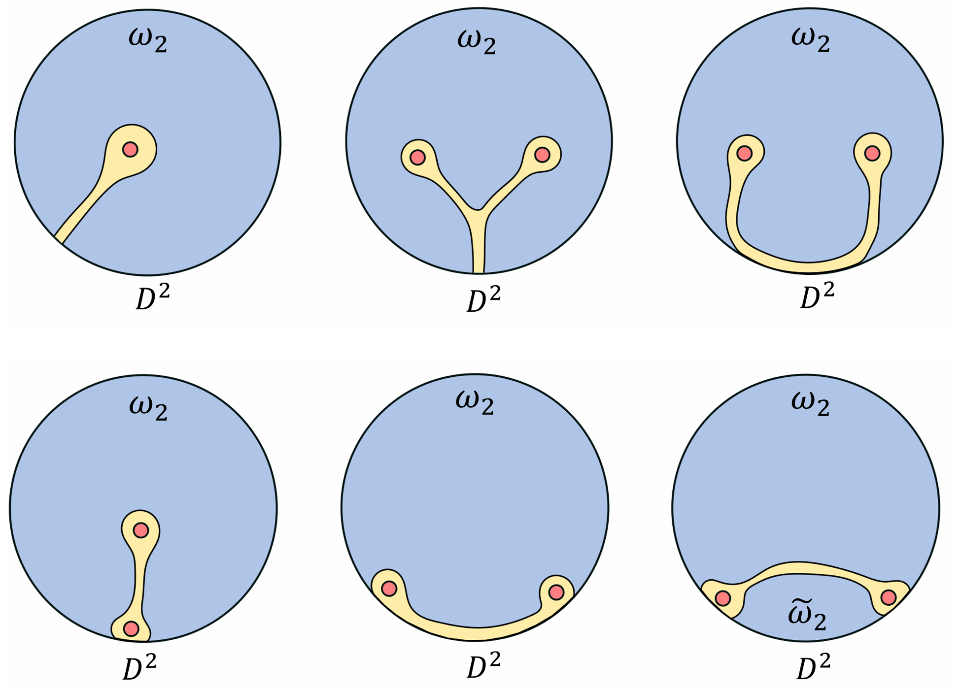
Refer to caption
Figure 15: A system on a disk D2D^{2}. Excitations are in the red area, which is a subset of the yellow region ω¯2\bar{\omega}_{2} (or ω¯2∩ω~¯2\bar{\omega}_{2}\cap\bar{\tilde{\omega}}_{2} for the last diagram). Using the HJW theorem, one can show there must be a unitary operator supported on the yellow region ω¯2\bar{\omega}_{2} (or ω¯2∩ω~¯2\bar{\omega}_{2}\cap\bar{\tilde{\omega}}_{2}) which creates the excitations.

Now let us consider a system on a disk D2D^{2}. The results are illustrated in Fig. 15. The proof is quite similar to that discussed above, the only difference is that we now need the result Σ(ω2)={σω21≡trω¯2|ψ⟩⟨ψ|}\Sigma(\omega_{2})=\{\sigma^{1}_{\omega_{2}}\equiv tr_{\bar{\omega}_{2}}|\psi\rangle\langle\psi|\}. Here ω2\omega_{2} is a simply connected subsystem attached to the boundary at one piece, see Fig. 9 and Sec. IV.2.3. |ψ⟩|\psi\rangle now represents the unique ground state on D2D^{2}. (For the last diagram, Σ(ω2∪ω~2)={σω2∪ω~21≡trω¯2∩ω~¯2|ψ⟩⟨ψ|}\Sigma(\omega_{2}\cup\tilde{\omega}_{2})=\{\sigma^{1}_{\omega_{2}\cup\tilde{\omega}_{2}}\equiv tr_{\bar{\omega}_{2}\cap\bar{\tilde{\omega}}_{2}}|\psi\rangle\langle\psi|\} is needed, where ω~2\tilde{\omega}_{2} has the same topology as ω2\omega_{2}.)

A new feature is that now a generic excited state with localized excitations need to be created using a process that involves the boundary, i.e. |φ⟩≠Ub​u​l​k​|ψ⟩|\varphi\rangle\neq U_{bulk}|\psi\rangle in general. Here Ub​u​l​kU_{bulk} is a unitary operator supported on a bulk subsystem.

Explicitly, single excitation away from the boundary of D2D^{2} can be created by a unitary operator supported on a string attached to the boundary. The string could be deformed, and the string can end at anywhere of the boundary. Unlike a single excitation on S2S^{2}, this single excitation on D2D^{2} may carry nontrivial bulk superselection sector. On the other hand, a single excitation located along the boundary can always be created by a local unitary operator acting around the excitation and therefore it carries a trivial boundary superselection sector. A pair of excitations away from the boundary of D2D^{2} could be created by a unitary operator supported on a stringlike region attached to the boundary. Note that there is no guarantee that the pair of excitations could be created by a unitary operator supported on a bulk string. Indeed, for some non-Abelian models, there can be an excited state |φ⟩|\varphi\rangle with a bulk anyon pair (a,a¯)(a,\bar{a}) located away from the boundary, but |φ⟩≠Ub​u​l​k​|ψ⟩|\varphi\rangle\neq U_{bulk}|\psi\rangle, see Sec. V.5 for more details. A pair of excitations around the boundary could be created by a unitary operator supported on a string along the boundary. The middle part of the string can be deformed into the bulk.

IV.3.2 Unitary string operators which create excitations of all possible superselection sectors

We have identified possible string types that connect pointlike excitations. Here, we discuss what type of string operators could guarantee the excitations to have all possible superselection sectors. One way is to do the explicit calculation using ribbon operators, see Sec. IV.5 and Sec. IV.6. Here, we discuss an alternative way which is applicable to models whose ribbon operators are hard (if not impossible) to be written down.

Refer to caption
Figure 16: An illustration of subsystems used in the proof, Ω1⊆Ω1′\Omega_{1}\subseteq\Omega_{1}^{\prime}, Ω2⊆Ω2′\Omega_{2}\subseteq\Omega_{2}^{\prime} and the red areas are excitations.
Theorem IV.1.

For a quantum double on S2S^{2} and an annulus subsystem Ω1\Omega_{1}, every extremal point of Σ⁡(Ω1)\Sigma(\Omega_{1}) can be written as t​rΩ¯1​|φ⟩​⟨φ|tr_{\bar{\Omega}_{1}}|\varphi\rangle\langle\varphi|. Here, |φ⟩|\varphi\rangle is an excited state with a pair of pointlike excitations, created by a unitary operator supported on a deformable bulk string crossing Ω1\Omega_{1}.

Proof.

We have shown that an excited state with a pair of excitations could be written as |φ⟩=U​|ψ⟩|\varphi\rangle=U|\psi\rangle. Here, |ψ⟩|\psi\rangle is the unique ground state on S2S^{2} and UU is supported on a deformable string. Also, one can always make a “thicker” annulus Ω1′\Omega_{1}^{\prime} on S2S^{2} which covers the entire S2S^{2} except for two localized regions, see Fig. 16. Then, one can show that
1) Σ⁡(Ω1,Ω1′)=Σ⁡(Ω1)\Sigma(\Omega_{1},\Omega_{1}^{\prime})=\Sigma(\Omega_{1}) using the explicit reduced density matrix in Sec. IV.2.2 and tracing out some suitable subsystems.
2) Each extremal point of Σ⁡(Ω1,Ω1′)\Sigma(\Omega_{1},\Omega_{1}^{\prime}) has purification on the system. This can be deduced from proposition III.4.

Therefore, there exists an excited state |φa⟩|\varphi^{a}\rangle with a pair of pointlike excitations in Ω¯1′\bar{\Omega}_{1}^{\prime} which could be created using a unitary string operator and it prepares an extremal point σΩ1a∈Σ⁡(Ω1)\sigma^{a}_{\Omega_{1}}\in\Sigma(\Omega_{1}), i.e. σΩ1a=t​rΩ¯1​|φa⟩​⟨φa|\sigma^{a}_{\Omega_{1}}=tr_{\bar{\Omega}_{1}}|\varphi^{a}\rangle\langle\varphi^{a}|. ∎

This also gives a natural way to define the superselection sector of pointlike excitations, i.e. by looking at what reduced density matrix of Σ⁡(Ω1)\Sigma(\Omega_{1}) it prepares. If it prepares an extremal point σΩ1a\sigma^{a}_{\Omega_{1}}, then the excitation circled by the annulus is in the aa superselection sector. If it prepares a nonextremal point, then it carries a superposition (or mixture) of superselection sectors.

Theorem IV.2.

For a quantum double on D2D^{2} and a subsystem Ω2\Omega_{2}, every extremal point of Σ⁡(Ω2)\Sigma(\Omega_{2}) can be written as t​rΩ¯2​|φ⟩​⟨φ|tr_{\bar{\Omega}_{2}}|\varphi\rangle\langle\varphi|. Here |φ⟩|\varphi\rangle is an excited state with a pair of pointlike excitations along the boundary, created by a unitary operator supported on a string along the boundary crossing Ω2\Omega_{2}. The middle part of the string can be deformed into the bulk.

Proof.

We have shown that an excited state with a pair of excitations along the boundary could be written as |φ⟩=U​|ψ⟩|\varphi\rangle=U|\psi\rangle. Here |ψ⟩|\psi\rangle is the unique ground state on D2D^{2} and UU is supported on a string along the boundary, the middle part of which could be deformed into the bulk. Also, one can always make a “thicker” annulus Ω2′\Omega_{2}^{\prime} on D2D^{2} which covers the entire D2D^{2} except for two localized regions along the boundary, see Fig. 16. Then, one can show:
1) Σ⁡(Ω2,Ω2′)=Σ⁡(Ω2)\Sigma(\Omega_{2},\Omega_{2}^{\prime})=\Sigma(\Omega_{2}) using the explicit reduced density matrix in Sec. IV.2.4 and tracing out some suitable subsystems.
2) Each extremal point of Σ⁡(Ω2,Ω2′)\Sigma(\Omega_{2},\Omega_{2}^{\prime}) has purification on the system. This can be deduced from Proposition III.4.

Therefore, there exists an excited state |φα⟩|\varphi^{\alpha}\rangle with a pair of pointlike excitations in Ω¯2′\bar{\Omega}_{2}^{\prime} which could be created using a unitary string operator along the boundary and it prepare an extremal point σΩ2α∈Σ⁡(Ω2)\sigma^{\alpha}_{\Omega_{2}}\in\Sigma(\Omega_{2}), i.e. σΩ2α=t​rΩ¯2​|φα⟩​⟨φα|\sigma^{\alpha}_{\Omega_{2}}=tr_{\bar{\Omega}_{2}}|\varphi^{\alpha}\rangle\langle\varphi^{\alpha}|. ∎

Similar to the bulk case, one could define a boundary superselection sector of the excitations using the element of Σ⁡(Ω2)\Sigma(\Omega_{2}) they prepare.

Theorem IV.3.

For a quantum double on D2D^{2} and a bulk annulus Ω1\Omega_{1}, every extremal point of Σ⁡(Ω1)\Sigma(\Omega_{1}) can be written as t​rΩ¯1​|φ⟩​⟨φ|tr_{\bar{\Omega}_{1}}|\varphi\rangle\langle\varphi|. Here |φ⟩|\varphi\rangle is an excited state with a pair of pointlike excitations in the bulk, created by a unitary operator supported on a bulk string crossing Ω1\Omega_{1}.

Proof.

First, note the fact that the ground state of S2S^{2} or D2D^{2} has the same reduced density matrix on a disklike subsystem in the bulk. In other words, a disk in the bulk could not tell whether it lives on S2S^{2} or D2D^{2}. One can choose a disklike subsystem containing the annulus Ω1\Omega_{1} and apply a bulk string operator inside the disklike subsystem, then, use Theorem IV.1 to finish the proof. ∎

IV.4 Topological entanglement entropy from topological invariant structures of information convex

Topological entanglement entropy (TEE) [10, 16] is an important topological invariant characterization of the ground state. In the middle steps of our derivation of Σ⁡(ω1)\Sigma(\omega_{1}), one could see the topological contribution explicitly, e.g. the −ln⁡|G|-\ln|G| in Eq. (39) for the bulk 33 3 The −ln⁡|G|+ln⁡|K|-\ln|G|+\ln|K| in Eq. (52) may also be regarded as a topological contribution for a system attached to a boundary, but in order to extract this contribution using a linear combination canceling out local contributions of entanglement entropy, one needs more than one boundary type.. However, in the final step, when we keep only topological invariant structures of Σ⁡(ω1)\Sigma(\omega_{1}), the important constant is lost.

Nevertheless, we show that TEE can be recovered as a lower bound (which appears to be saturated), given the topological invariant structures of Σ⁡(ω1)\Sigma(\omega_{1}) and Σ⁡(Ω1)\Sigma(\Omega_{1}). In fact, the lower bound always saturates given a few simple assumptions [30]. In this sense, TEE is retained in the topological invariant structures of information convex.

Below is the derivation of the lower bound. First, recall some properties of Σ⁡(Ω1)\Sigma(\Omega_{1}):

Σ⁡(Ω1)={σΩ1|σΩ1=∑apa​σΩ1a}withS⁡(σΩ1a)=S⁡(σΩ11)+ln⁡da2,σΩ1a⋅σΩ1b=0fora≠b.\Sigma({\Omega_{1}})=\{\sigma_{\Omega_{1}}|\sigma_{\Omega_{1}}=\sum_{a}p_{a}\,\sigma^{a}_{\Omega_{1}}\}\quad\textrm{with}\quad S(\sigma^{a}_{\Omega_{1}})=S(\sigma^{1}_{\Omega_{1}})+\ln d^{2}_{a},\qquad\sigma^{a}_{\Omega_{1}}\cdot\sigma^{b}_{\Omega_{1}}=0\quad\textrm{for}\quad a\neq b. (66)

From these properties, one could calculate the entanglement entropy for any σΩ1∈Σ⁡(Ω1)\sigma_{\Omega_{1}}\in\Sigma(\Omega_{1}) and find the element σ~Ω1∈Σ⁡(Ω1)\tilde{\sigma}_{\Omega_{1}}\in\Sigma(\Omega_{1}) with the maximal entanglement entropy:

S⁡(∑apa​σΩ1a)\displaystyle S(\sum_{a}p_{a}\,\sigma^{a}_{\Omega_{1}}) =\displaystyle= ∑a(pa​S​(σΩ1a)−pa​ln⁡pa)\displaystyle\sum_{a}\big(p_{a}\,S(\sigma^{a}_{\Omega_{1}})-p_{a}\ln p_{a}\big) (67)
=\displaystyle= S⁡(σΩ11)+∑apa​ln⁡(da2pa)\displaystyle S(\sigma^{1}_{\Omega_{1}})+\sum_{a}p_{a}\ln\bigg(\frac{d_{a}^{2}}{p_{a}}\bigg)
≤\displaystyle\leq S⁡(σΩ11)+ln⁡𝒟2“=” iff ​pa=da2𝒟2\displaystyle S(\sigma^{1}_{\Omega_{1}})+\ln\mathcal{D}^{2}\qquad\qquad\qquad\textrm{``=" iff }p_{a}=\frac{d_{a}^{2}}{\mathcal{D}^{2}}
⇒σ~Ω1\displaystyle\Rightarrow\quad\tilde{\sigma}_{\Omega_{1}} =\displaystyle= ∑ada2𝒟2​σΩ1a.\displaystyle\sum_{a}\frac{d_{a}^{2}}{\mathcal{D}^{2}}\,\sigma^{a}_{\Omega_{1}}. (68)

Here 𝒟=∑ada2\mathcal{D}=\sqrt{\sum_{a}d_{a}^{2}} is the total quantum dimension. It is obvious that S⁡(σ~Ω1)−S⁡(σΩ11)=ln⁡𝒟2S(\tilde{\sigma}_{\Omega_{1}})-S(\sigma^{1}_{\Omega_{1}})=\ln\mathcal{D}^{2} is a topological invariance. Similar constructions apply to other subsystem topologies.

Refer to caption
Figure 17: Divide Ω1\Omega_{1} into A,B,CA,B,C.

Now, let us divide Ω1\Omega_{1} into subsystems A,B,CA,B,C shown in Fig. 17 and take the Levin-Wen definition of topological entanglement entropy [16] (an overall minus sign is added):

St​o​p​o=(SA​B+SB​C−SB−SA​B​C)|σ1=I(A:C|B)|σ1.S_{topo}=(S_{AB}+S_{BC}-S_{B}-S_{ABC})|_{\sigma^{1}}=I(A:C|B)|_{\sigma^{1}}. (69)

Here σ1=|ψ⟩​⟨ψ|\sigma^{1}=|\psi\rangle\langle\psi| is the ground-state density matrix and I(A:C|B)≡SA​B+SB​C−SB−SA​B​CI(A:C|B)\equiv S_{AB}+S_{BC}-S_{B}-S_{ABC} is the conditional mutual information. According to the strong subadditivity I(A:C|B)≥0I(A:C|B)\geq 0 is true in general. Also, all reduced density matrices in Σ⁡(Ω1)\Sigma(\Omega_{1}) have the same reduced density matrix on A​BAB, B​CBC [for a proof, use the structure of Σ⁡(ω1)\Sigma(\omega_{1}), and that A​BAB and B​CBC are of the same topology type as ω1\omega_{1}]. Therefore,

{σ~A​B=σA​B1σ~B​C=σB​C1⇒I(A:C|B)|σ1\displaystyle\left\{\begin{array}[]{l}\tilde{\sigma}_{AB}=\sigma^{1}_{AB}\\ \tilde{\sigma}_{BC}=\sigma^{1}_{BC}\end{array}\right.\quad\Rightarrow\quad I(A:C|B)|_{\sigma^{1}} =\displaystyle= I(A:C|B)|σ~+S(σ~Ω1)−S(σΩ11)\displaystyle I(A:C|B)|_{\tilde{\sigma}}+S(\tilde{\sigma}_{\Omega_{1}})-S(\sigma^{1}_{\Omega_{1}})
=\displaystyle= I(A:C|B)|σ~+ln𝒟2\displaystyle I(A:C|B)|_{\tilde{\sigma}}+\ln\mathcal{D}^{2}
≥\displaystyle\geq ln⁡𝒟2\displaystyle\ln\mathcal{D}^{2}
⇒St​o​p​o\displaystyle\Rightarrow\quad S_{topo} ≥\displaystyle\geq ln𝒟2“=” iff I(A:C|B)|σ~=0.\displaystyle\ln\mathcal{D}^{2}\qquad\qquad\qquad\textrm{``=" iff }I(A:C|B)|_{\tilde{\sigma}}=0. (73)

Comparing with the knowledge of TEE, the lower bound appears to be saturated and therefore I(A:C|B)|σ~=0I(A:C|B)|_{\tilde{\sigma}}=0. This result may be regarded as a generalization of our previous lower bound [40] into the non-Abelian case. We are aware that the reduced density matrix with maximal entanglement entropy σ~Ω1∈Σ⁡(Ω1)\tilde{\sigma}_{\Omega_{1}}\in\Sigma(\Omega_{1}) has zero conditional mutual information if the simple assumptions (I) and (II) in Ref. [30] are satisfied. The assumptions are indeed satisfied for the ground states of exactly solved models for topological orders. On the other hand, given arbitrary ρA​B​C\rho_{ABC}, it is in general not possible [41] to find a σA​B​C\sigma_{ABC} such that: (1) σA​B=ρA​B\sigma_{AB}=\rho_{AB}, (2) σB​C=ρB​C\sigma_{BC}=\rho_{BC}, and (3) I(A:C|B)|σ=0I(A:C|B)|_{\sigma}=0.

To summarize,

St​o​p​o=S⁡(σ~Ω1)−S⁡(σΩ11)=ln⁡𝒟2.S_{topo}=S(\tilde{\sigma}_{\Omega_{1}})-S(\sigma^{1}_{\Omega_{1}})=\ln\mathcal{D}^{2}. (74)

This is true for exactly solved models satisfying (I) and (II) assumptions in Ref. [30]. There are evidences and beliefs that St​o​p​oS_{topo} is robust under generic local perturbations (which could be treated as finite depth quantum circuits), although very special examples like the Bravyi’s counterexample [42] could change St​o​p​oS_{topo}. It might be interesting to study the stability of S⁡(σΩ1a)−S⁡(σΩ11)S({\sigma^{a}_{\Omega_{1}}})-S(\sigma^{1}_{\Omega_{1}}), S⁡(σ~Ω1)−S⁡(σΩ11)S({\tilde{\sigma}}_{\Omega_{1}})-S(\sigma^{1}_{\Omega_{1}}) and their generalizations.

IV.5 Bulk ribbon operators

Let us review bulk ribbon operators and the bulk topological excitations (bulk anyons) it creates. The review is brief and focusing on properties useful in our calculations. For more details, we refer to Refs. [7, 13, 20].

A bulk ribbon operator Fξh,gF_{\xi}^{h,g} is defined for an open ribbon ξ\xi in the bulk (bulk ribbon) and h,g∈Gh,g\in G. See Fig. 18 for a bulk ribbon connecting bulk sites s0s_{0} and s1s_{1}. Let |φξh,g⟩≡Fξh,g​|ψ⟩|\varphi^{h,g}_{\xi}\rangle\equiv F^{h,g}_{\xi}|\psi\rangle (not normalized). One can show |φξh,g⟩|\varphi^{h,g}_{\xi}\rangle has eigenvalues Bf=1B_{f}=1, Av=1A_{v}=1, Av′K=1A_{v^{\prime}}^{K}=1 for all f,vf,v that are not contained in s0,s1s_{0},s_{1} and for all v′v^{\prime}. In other words, Fξh,gF_{\xi}^{h,g} (when acting on a ground state or a state locally minimizing energy) could create excitations only on s0s_{0} and s1s_{1}. It is known that ξ\xi can be topologically deformed, in the sense that two ribbons ξ\xi and ξ′\xi^{\prime} both connecting s0s_{0} and s1s_{1}, we have corresponding ribbon operators Fξh,gF_{\xi}^{h,g} and Fξ′h,gF_{\xi^{\prime}}^{h,g}, which are different operators, but Fξh,g​|ψ⟩=Fξ′h,g​|ψ⟩F^{h,g}_{\xi}|\psi\rangle=F^{h,g}_{\xi^{\prime}}|\psi\rangle.

The bulk ribbon operators have basic properties

(Fξh,g)†=Fξh¯,g,Fξh,g​Fξh′,g′=δg,g′​Fξh​h′,g.(F^{h,g}_{\xi})^{\dagger}=F^{\bar{h},g}_{\xi},\qquad\qquad F^{h,g}_{\xi}F^{h^{\prime},g^{\prime}}_{\xi}=\delta_{g,g^{\prime}}F^{hh^{\prime},g}_{\xi}. (75)

For ξ=ξ1​ξ2\xi=\xi_{1}\xi_{2}, we have the “gluing relation:”

Fξ1​ξ2h,g=∑l∈GFξ1h,l​Fξ2l¯​h​l,l¯​g.F^{h,g}_{\xi_{1}\xi_{2}}=\sum_{l\in G}F_{\xi_{1}}^{h,l}F_{\xi_{2}}^{\bar{l}hl,\bar{l}g}. (76)
Refer to caption
Figure 18: Bulk ribbon operators and boundary ribbon operators. (a) Fξh,gF^{h,g}_{\xi}, h,g∈Gh,g\in G is a bulk ribbon operator. ξ\xi is a bulk ribbon consisting of bulk links and x1,x2,x3,x4,y1,y2,y3∈Gx_{1},x_{2},x_{3},x_{4},y_{1},y_{2},y_{3}\in G. (b) Iζh,kI^{h,k}_{\zeta}, h∈Gh\in G and k∈Kk\in K is a boundary ribbon operator. ζ\zeta is a boundary ribbon (for KK boundary) consisting of both boundary links with x1,x2,x3,x4∈Kx_{1},x_{2},x_{3},x_{4}\in K and bulk links with y1,y2,y3∈Gy_{1},y_{2},y_{3}\in G.

Change of basis: {Fξh,g}→{Fξ(c,R)​(u,v)}\{F^{h,g}_{\xi}\}\rightarrow\{F_{\xi}^{(c,R)(u,v)}\}:

Fξ(c,R)​(u,v)=∑t∈E⁡(c)Γ¯Rj​j′​(t)​Fξc¯i,pi​t​p¯i′.F^{(c,R)(u,v)}_{\xi}=\sum_{t\in E(c)}\bar{\Gamma}_{R}^{jj^{\prime}}(t)F_{\xi}^{\bar{c}_{i},p_{i}t\bar{p}_{i^{\prime}}}. (77)

Here,
1) c∈(G)c​jc\in(G)_{cj}, i.e. c={g​rc​g¯|g∈G}c=\{g\,r_{c}\,\bar{g}\,|\,g\in G\} and rcr_{c} is a representative of cc.
2) E⁡(c)E(c) is the centralizer group of cc, defined as E⁡(c)≡{g∈G|g​rc=rc​g}E(c)\equiv\{g\in G\,|\,g\,r_{c}=r_{c}\,g\}.
3) R∈(E⁡(c))i​rR\in(E(c))_{ir} and nRn_{R} is the dimension of RR. ΓR\Gamma_{R} is the unitary nR×nRn_{R}\times n_{R} matrix associated with RR, with components ΓRj​j′{\Gamma}_{R}^{jj^{\prime}}. Γ¯Rj​j′\bar{\Gamma}_{R}^{jj^{\prime}} is the complex conjugate of ΓRj​j′{\Gamma}_{R}^{jj^{\prime}}.
4) P⁡(c)={pi}i=1|c|P(c)=\{p_{i}\}_{i=1}^{|c|} is a set of representatives of G/E⁡(c)G/E(c). c={ci}i=1|c|c=\{c_{i}\}_{i=1}^{|c|} with ci=pi​rc​p¯ic_{i}=p_{i}r_{c}\bar{p}_{i}.
5) u=(i,j),v=(i′,j′)u=(i,j),v=(i^{\prime},j^{\prime}) with i,i′=1,⋯,|c|i,i^{\prime}=1,\cdots,|c| and j,j′=1,⋯,nRj,j^{\prime}=1,\cdots,n_{R}.
For more explanations of the notation, see Appendix A.1.

Note that we picked a normalization such that the “gluing relation” in this basis looks simple:

Fξ1​ξ2(c,R)​(u,v)=∑wFξ1(c,R)​(u,w)​Fξ2(c,R)​(w,v),F_{\xi_{1}\xi_{2}}^{(c,R)(u,v)}=\sum_{w}F_{\xi_{1}}^{(c,R)(u,w)}F_{\xi_{2}}^{(c,R)(w,v)}, (78)

where w=(i′′,j′′)w=(i^{\prime\prime},j^{\prime\prime}). For a (open) bulk ribbon ξ\xi:

tr(Fξh,gσξ1)=1|G|δ1,h⇒tr(Fξ(c,R)(u,v)†Fξ(c′,R′)​(u′,v′)σξ1)=δc,c′δR,R′δu,u′δv,v′1|c|⋅nR.tr\bigg(F^{h,g}_{\xi}\sigma^{1}_{\xi}\bigg)=\frac{1}{|G|}\delta_{1,h}\quad\Rightarrow\quad tr\bigg(F_{\xi}^{(c,R)(u,v)\dagger}F_{\xi}^{(c^{\prime},R^{\prime})(u^{\prime},v^{\prime})}\sigma^{1}_{\xi}\bigg)=\delta_{c,c^{\prime}}\delta_{R,R^{\prime}}\delta_{u,u^{\prime}}\delta_{v,v^{\prime}}\,\frac{1}{|c|\cdot n_{R}}. (79)

Here σξ1\sigma^{1}_{\xi} is the ground-state reduced density matrix on the ribbon ξ\xi. σξ1\sigma^{1}_{\xi} is proportional to the identity unless there are AvgA^{g}_{v} or BfB_{f} supported on ξ\xi, Eq. (79) is true for both cases. This formula will be useful in the calculation of the reduced density matrix.

For non-Abelian GG, the ribbon operators Fξ(c,R)​(u,v)F^{(c,R)(u,v)}_{\xi} are not unitary in general, but there are corresponding unitary operators. In addition to the theorems in Sec. IV.3, explicit ribbon calculations can be done. From Eq. (79), using the explicit wavefunction of the ground state |ψ⟩|\psi\rangle and the HJW theorem, one can show

|φξ(c,R)​(u,v)⟩≡|c|⋅nR​Fξ(c,R)​(u,v)​|ψ⟩=U⁡(ξ)​|ψ⟩.|\varphi_{\xi}^{(c,R)(u,v)}\rangle\equiv\sqrt{|c|\cdot n_{R}}\,F_{\xi}^{(c,R)(u,v)}|\psi\rangle=U(\xi)|\psi\rangle. (80)

Here, U⁡(ξ)U(\xi) is a unitary operator supported on a stringlike region within a few lattice spacings to ξ\xi. Note that the support of U⁡(ξ)U(\xi) can be slightly fatter than ξ\xi. This result is independent from whether the system has boundaries or not, the only requirement is that ξ\xi can be contained in a disklike subsystem in the bulk.

IV.6 Boundary ribbon operators

Let us consider a new type of ribbon operator Iζh,kI_{\zeta}^{h,k} with h∈Gh\in G, k∈Kk\in K defined for open ribbon ζ\zeta that lies along the boundary (boundary ribbon), see Fig. 18 for a boundary ribbon connecting boundary sites s0′s^{\prime}_{0} and s1′s^{\prime}_{1}. Very similar to bulk ribbon operators, Iζh,kI_{\zeta}^{h,k} can create excitations only at s0′s^{\prime}_{0} and s1′s^{\prime}_{1} (when acting on a ground state or a state locally minimizing energy).

The boundary ribbon operators have the basic properties:

(Iζh,k)†=Iζh¯,k,Iζh,k​Iζh′,k′=δk,k′​Iζh​h′,k.(I^{h,k}_{\zeta})^{\dagger}=I_{\zeta}^{\bar{h},k},\qquad\qquad I^{h,k}_{\zeta}I^{h^{\prime},k^{\prime}}_{\zeta}=\delta_{k,k^{\prime}}\,I^{hh^{\prime},k}_{\zeta}. (81)

The “gluing relation” can be written as:

Iζ1​ζ2h,k=∑l∈KIζ1h,l​Iζ2l¯​h​l,l¯​k.I_{\zeta_{1}\zeta_{2}}^{h,k}=\sum_{l\in K}I_{\zeta_{1}}^{h,l}I_{\zeta_{2}}^{\bar{l}hl,\bar{l}k}. (82)

Let us consider a linear combination: {Iζh,k}→{Iζ(T,R)​(u,v)}\{I^{h,k}_{\zeta}\}\rightarrow\{I_{\zeta}^{(T,R)(u,v)}\}:

Iζ(T,R)​(u,v)≡∑t∈KrTΓ¯Rj​j′​(t)​Iζsi,qi​t​q¯i′.I^{(T,R)(u,v)}_{\zeta}\equiv\sum_{t\in K^{r_{T}}}\bar{\Gamma}^{jj^{\prime}}_{R}(t)I_{\zeta}^{{s}_{i},q_{i}t\bar{q}_{i^{\prime}}}. (83)

Here,
1) T∈K\G/KT\in K\backslash G/K is a double coset, i.e. T={k1rTk2|k1,k2∈K}T=\{k_{1}r_{T}k_{2}\,|\,k_{1},k_{2}\in K\}. rT∈Gr_{T}\in G is a representative of TT.
2) KrT≡K​⋂rT​K​r¯TK^{r_{T}}\equiv K\bigcap r_{T}K\bar{r}_{T} is a subgroup of KK, and it depends on the choice of rTr_{T} in general.
3) R∈(KrT)i​rR\in(K^{r_{T}})_{ir} and nRn_{R} is the dimension of RR. ΓR\Gamma_{R} is the unitary nR×nRn_{R}\times n_{R} matrix associated with RR, with components ΓRj​j′{\Gamma}_{R}^{jj^{\prime}}. Γ¯Rj​j′\bar{\Gamma}_{R}^{jj^{\prime}} is the complex conjugate of ΓRj​j′{\Gamma}_{R}^{jj^{\prime}}.
4) Q={qi}Q=\{q_{i}\}, i=1,⋯,|Q|i=1,\cdots,|Q| is a set of representatives of K/KrTK/K^{r_{T}}. |Q|=|K|/|KrT|=|T|/|K||Q|=|K|/|K^{r_{T}}|=|T|/|K|. si≡qi​rT​q¯is_{i}\equiv q_{i}r_{T}\bar{q}_{i}.
5) u=(i,j)u=(i,j), v=(i′,j′)v=(i^{\prime},j^{\prime}) with i,i′=1,⋯,|Q|i,i^{\prime}=1,\cdots,|Q| and j,j′=1,⋯,nRj,j^{\prime}=1,\cdots,n_{R}.
For more explanations of the notation, see Appendix A.1.

Note that, for a set of chosen rTr_{T}, the set {Iζ(T,R)​(u,v)}\{I_{\zeta}^{(T,R)(u,v)}\} may contain a smaller number of elements than {Iζh,k}\{I^{h,k}_{\zeta}\}. We need to be careful to say it is a change of basis. For K={1}K=\{1\}, it is a change of basis.

Remark.

Our boundary ribbon operators Iζ(T,R)​(u,v)I_{\zeta}^{(T,R)(u,v)} are fundamentally different from the Yρ(T,R)​(u,v)Y_{\rho}^{(T,R)(u,v)} operators considered in Ref. [27]. The operator Iζ(T,R)​(u,v)I_{\zeta}^{(T,R)(u,v)} is defined for a ribbon ζ\zeta that lies along the boundary, while the operator Yρ(T,R)​(u,v)Y_{\rho}^{(T,R)(u,v)} is defined for ribbon ρ\rho inside the boundary. Unlike the model in Ref. [27], our model does not have Hilbert space for the interior of a boundary. Therefore, the excitations created by Yρ(T,R)​(u,v)Y_{\rho}^{(T,R)(u,v)} operator are not defined in our model. On the other hand, the excitation created by Iζ(T,R)​(u,v)I_{\zeta}^{(T,R)(u,v)} can be defined not only in our model but also in the models of Ref. [20, 27]. The excitations created by Iζ(T,R)​(u,v)I_{\zeta}^{(T,R)(u,v)} are deconfined topological excitations (parallel to the topological excitations created by Fξ(c,R)​(u,v)F_{\xi}^{(c,R)(u,v)} in the bulk). The middle part of the boundary ribbon ζ\zeta can be deformed into the bulk. The excitations created by Yρ(T,R)​(u,v)Y_{\rho}^{(T,R)(u,v)} are confined, and the energy cost is proportional to the length of the ribbon ρ\rho. The ribbon operator Yρ(T,R)​(u,v)Y_{\rho}^{(T,R)(u,v)} cannot be deformed.

One could verify that

tr(Iζh,kσζ1)=1|K|δ1,h⇒tr(Iζ(T,R)(u,v)†Iζ(T′,R′)​(u′,v′)σζ1)=|KrT|nR⋅|K|δT,T′δR,R′δu,u′δv,v′.tr\bigg(I_{\zeta}^{h,k}\sigma^{1}_{\zeta}\bigg)=\frac{1}{|K|}\delta_{1,h}\quad\Rightarrow\quad tr\bigg(I_{\zeta}^{(T,R)(u,v)\dagger}I_{\zeta}^{(T^{\prime},R^{\prime})(u^{\prime},v^{\prime})}\sigma^{1}_{\zeta}\bigg)=\frac{|K^{r_{T}}|}{n_{R}\cdot|K|}\delta_{T,T^{\prime}}\delta_{R,R^{\prime}}\delta_{u,u^{\prime}}\delta_{v,v^{\prime}}. (84)

Here, σζ1\sigma^{1}_{\zeta} is the ground-state reduced density matrix on ζ\zeta. σζ1\sigma^{1}_{\zeta} is generally not proportional to the identity unless K={1}K=\{1\} since for K≠{1}K\neq\{1\}, and for a ζ\zeta not too short, it must contain some AvkA^{k}_{v} with k≠1k\neq 1.

It turns out that the nice “gluing relation” parallel to Eq. (78) only appears for boundary ribbon operators with one additional constraint of TT and rTr_{T}, i.e. if there is a choice of rT∈Tr_{T}\in T such that rT​m=m​rTr_{T}m=mr_{T} for ∀m∈KrT\forall m\in K^{r_{T}}. When choosing this rTr_{T}, using Eqs. (82,83), one derives

Iζ1​ζ2(T,R)​(u,v)=∑wIζ1(T,R)​(u,w)​Iζ2(T,R)​(w,v)ifrT​m=m​rT∀m∈KrT,I^{(T,R)(u,v)}_{\zeta_{1}\zeta_{2}}=\sum_{w}I^{(T,R)(u,w)}_{\zeta_{1}}I^{(T,R)(w,v)}_{\zeta_{2}}\quad\qquad\textrm{if}\quad r_{T}m=mr_{T}\quad\forall m\in K^{r_{T}}, (85)

where w=(i′′,j′′)w=(i^{\prime\prime},j^{\prime\prime}). This condition (and therefore Eq. (85)) holds for a large class of boundaries including
1) K={1}K=\{1\} boundary for a general GG quantum double.
2) K=GK=G boundary for a general GG quantum double.

The operators Iζ(T,R)​(u,v)I_{\zeta}^{(T,R)(u,v)} are not unitary in general, but there exist corresponding unitary operators:

|φζ(T,R)​(u,v)⟩≡nR⋅|K||KrT|​Iζ(T,R)​(u,v)​|ψ⟩=U⁡(ζ)​|ψ⟩.|\varphi^{(T,R)(u,v)}_{\zeta}\rangle\equiv\sqrt{\frac{n_{R}\cdot|K|}{|K^{r_{T}}|}}\,I_{\zeta}^{(T,R)(u,v)}|\psi\rangle=U(\zeta)|\psi\rangle. (86)

Here, U⁡(ζ)U(\zeta) is a unitary operator supported on a stringlike region within a few lattice spacings to ζ\zeta. Note that the support of U⁡(ζ)U(\zeta) can be slightly fatter than ζ\zeta. This result has been proved (up to normalization) in Sec. IV.3.1, and it can be shown by explicit calculation using Eq. (84), the explicit wave function of the ground state |ψ⟩|\psi\rangle and the HJW theorem. This calculation also determines the overall normalization.

IV.7 Bulk ribbon operators and the extremal points of Σ⁡(Ω1)\Sigma(\Omega_{1})

Let us consider the Ω1\Omega_{1} subsystem discussed earlier in Sec. IV.2. We show (with explicit calculation) that a pair of topological excitations (here are bulk anyons) (a,a¯)(a,\bar{a}) created by a bulk process prepare the extremal point σΩ1a∈Σ⁡(Ω1)\sigma^{a}_{\Omega_{1}}\in\Sigma(\Omega_{1}). This construction confirms that the extremal points of Σ⁡(Ω1)\Sigma(\Omega_{1}) are in one to one correspondence with bulk superselection sectors (bulk anyon types). Also, see theorem IV.3, for a powerful but less explicit way.

Refer to caption
Figure 19: The whole system is a disk D2D^{2}, and it is divided into subsystems A,Ω1,BA,\Omega_{1},B. The bulk ribbon ξ\xi connects bulk sites s0s_{0} and s1s_{1}. s0s_{0} is in AA and s1s_{1} is in CC. The ribbon ξ=ξ1​ξ2​ξ3\xi=\xi_{1}\xi_{2}\xi_{3} with ξ1⊆A\xi_{1}\subseteq A, ξ2⊆Ω1\xi_{2}\subseteq\Omega_{1}, and ξ3⊆B\xi_{3}\subseteq B.

Consider the process and bulk ribbon shown in Fig. 19, the bulk ribbon ξ=ξ1​ξ2​ξ3\xi=\xi_{1}\xi_{2}\xi_{3} connects bulk sites s0s_{0} and s1s_{1} that are separated by Ω1\Omega_{1}. Define the excited state (normalized) |φξ(c,R)​(u,v)⟩≡|c|⋅nR​Fξ(c,R)​(u,v)​|ψ⟩|\varphi^{(c,R)(u,v)}_{\xi}\rangle\equiv\sqrt{|c|\cdot n_{R}}\,F_{\xi}^{(c,R)(u,v)}|\psi\rangle. From our knowledge about bulk ribbon operators, |φξ(c,R)​(u,v)⟩|\varphi^{(c,R)(u,v)}_{\xi}\rangle has excitations only at the two ends of ξ\xi, i.e. s0s_{0} and s1s_{1}. Since s0s_{0} and s1s_{1} are away from Ω1\Omega_{1}, it is clear that t​rΩ¯1​|φξ(c,R)​(u,v)⟩​⟨φξ(c,R)​(u,v)|∈Σ⁡(Ω1)tr_{\bar{\Omega}_{1}}|\varphi^{(c,R)(u,v)}_{\xi}\rangle\langle\varphi^{(c,R)(u,v)}_{\xi}|\in\Sigma(\Omega_{1}).

Now let us calculate t​rΩ¯1​|φξ(c,R)​(u,v)⟩​⟨φξ(c,R)​(u,v)|tr_{\bar{\Omega}_{1}}|\varphi^{(c,R)(u,v)}_{\xi}\rangle\langle\varphi^{(c,R)(u,v)}_{\xi}|. From the “gluing relation” (78), one obtains

Fξ1​ξ2​ξ3(c,R)​(u,v)=∑w1,w2Fξ1(c,R)​(u,w1)​Fξ2(c,R)​(w1,w2)​Fξ3(c,R)​(w2,v).F_{\xi_{1}\xi_{2}\xi_{3}}^{(c,R)(u,v)}=\sum_{w_{1},w_{2}}F_{\xi_{1}}^{(c,R)(u,w_{1})}F_{\xi_{2}}^{(c,R)(w_{1},w_{2})}F_{\xi_{3}}^{(c,R)(w_{2},v)}. (87)

Let us write the ground state |ψ⟩|\psi\rangle as:

|ψ⟩=∑ha,Hb|{ha}⟩A|{ha},{Hb}⟩Ω1|{Hb}⟩B.|\psi\rangle=\sum_{h_{a},H_{b}}|\{h_{a}\}\rangle_{A}|\{h_{a}\},\{H_{b}\}\rangle_{\Omega_{1}}|\{H_{b}\}\rangle_{B}. (88)

Here, {ha}\{h_{a}\} with a=1,⋯,na=1,\cdots,n is a set of link configurations, ha∈Gh_{a}\in G. Similarly, {Hb}\{H_{b}\} with b=1,⋯,Nb=1,\cdots,N is a set of link configurations, Hb∈GH_{b}\in G. The state |{ha}⟩A|\{h_{a}\}\rangle_{A} is the unique equal weight superposition of all zero flux configurations determined by a set of {ha}\{h_{a}\} on ∂A\partial A. The zero flux requirement tells us that h1h2⋯hn=1h_{1}h_{2}\cdots h_{n}=1. Similarly, the states |{ha},{Hb}⟩Ω1|\{h_{a}\},\{H_{b}\}\rangle_{\Omega_{1}} and |{Hb}⟩B|\{H_{b}\}\rangle_{B} are the unique equal weight superposition of all zero flux configurations with fixed link values hah_{a} and HbH_{b} satisfying h1h2⋯hn=H1H2⋯HN=1h_{1}h_{2}\cdots h_{n}=H_{1}H_{2}\cdots H_{N}=1.

Then, one can calculate σΩ1​(c,R)≡t​rΩ¯1​|φξ(c,R)​(u,v)⟩​⟨φξ(c,R)​(u,v)|\sigma_{\Omega_{1}}(c,R)\equiv tr_{\bar{\Omega}_{1}}|\varphi_{\xi}^{(c,R)(u,v)}\rangle\langle\varphi_{\xi}^{(c,R)(u,v)}|, and find (up to normalization):

σΩ1(c,R)=∑w1,w2Fξ2(c,R)​(w1,w2)σΩ11Fξ2(c,R)(w1,w2)†.\sigma_{\Omega_{1}}(c,R)=\sum_{w_{1},w_{2}}\,F_{\xi_{2}}^{(c,R)(w_{1},w_{2})}\sigma^{1}_{\Omega_{1}}F_{\xi_{2}}^{(c,R)(w_{1},w_{2}){\dagger}}. (89)

Here, σΩ11=t​rΩ¯1​|ψ⟩​⟨ψ|\sigma^{1}_{\Omega_{1}}=tr_{\bar{\Omega}_{1}}|\psi\rangle\langle\psi| is the reduced density matrix of the ground state. To get the result above, we have used the fact that

⟨{ha}|Fξ1(c,R)(u,w1)†Fξ1(c,R)​(u,w~1)|{h~a}⟩AA=δh,h~trξ1(Fξ1(c,R)(u,w1)†Fξ1(c,R)​(u,w~1)σξ11)=δh,h~δw1,w~11nR⋅|c|.\,{}_{A}\langle\{h_{a}\}|F_{\xi_{1}}^{(c,R)(u,w_{1}){\dagger}}F_{\xi_{1}}^{(c,R)(u,\tilde{w}_{1})}|\{\tilde{h}_{a}\}\rangle_{A}=\delta_{h,\tilde{h}}\,tr_{\xi_{1}}\bigg(F_{\xi_{1}}^{(c,R)(u,w_{1}){\dagger}}F_{\xi_{1}}^{(c,R)(u,\tilde{w}_{1})}\sigma^{1}_{\xi_{1}}\bigg)=\delta_{h,\tilde{h}}\delta_{w_{1},\tilde{w}_{1}}\frac{1}{n_{R}\cdot|c|}. (90)

Here, σξ11\sigma^{1}_{\xi_{1}} is the reduced density matrix of the ground state on ξ1\xi_{1}. δh,h~\delta_{h,\tilde{h}} is short for ∏aδha,h~a\prod_{a}\delta_{h_{a},\tilde{h}_{a}}. There is a similar equation as Eq. (90) when replacing |{ha}⟩A|\{h_{a}\}\rangle_{A} by |{Hb}⟩B|\{H_{b}\}\rangle_{B} and replacing ξ1\xi_{1} by ξ3\xi_{3}. One could verify that the reduced density matrix σΩ1​(c,R)\sigma_{\Omega_{1}}(c,R) in Eq. (89) is identical to the extremal point σΩ1a\sigma_{\Omega_{1}}^{a}, with a=(c,R)a=(c,R). In other words, every extremal point of Σ⁡(Ω1)\Sigma(\Omega_{1}) can be obtained by an anyon process in the bulk shown in Fig. 19.

This further shows that Σ⁡(Ω1)=Σ⁡(Ω1,Ω1′)\Sigma(\Omega_{1})=\Sigma(\Omega_{1},\Omega_{1}^{\prime}), as long as Ω¯1′\bar{\Omega}^{\prime}_{1} contains s0s_{0} and s1s_{1}. Using Eqs. (78,79), the ground-state wave function and the HJW theorem one can show that each of the anyons a,a¯a,\bar{a} at the endpoints s0,s1s_{0},s_{1} can be moved by local unitary operators acting around s0s_{0} and s1s_{1}, respectively.

IV.8 Boundary ribbon operators and the extremal points of Σ⁡(Ω2)\Sigma(\Omega_{2})

Now consider the Ω2\Omega_{2} subsystem discussed in Sec. IV.2. As is shown in theorem IV.2, it is possible to create a pair of excitations along the boundary by a unitary string operator along the boundary and the excitations could carry any boundary superselection sector. On the other hand, it is nice to have explicit constructions. In practice, we find that explicit constructions are challenging beyond models with the additional requirement: for every T∈K\G/KT\in K\backslash G/K, there exists rT∈Tr_{T}\in T such that rT​m=m​rTr_{T}m=mr_{T} for ∀m∈KrT\forall m\in K^{r_{T}}, the same requirement for the “gluing relation” (85) to apply. The following constructions are restricted to models satisfying this requirement.

We show that a pair of topological excitations (α,α¯)(\alpha,\bar{\alpha}) created by a process involve the boundary prepare the extremal point σΩ2α∈Σ⁡(Ω2)\sigma^{\alpha}_{\Omega_{2}}\in\Sigma(\Omega_{2}), with α=(T,R)\alpha=(T,R). This construction confirms the fact that the extremal points of Σ⁡(Ω2)\Sigma(\Omega_{2}) have the same label as the boundary superselection sector.

Refer to caption
Figure 20: The whole system is a disk D2D^{2} and it is divided into subsystems A,Ω2,BA,\Omega_{2},B. The bulk ribbon ζ\zeta connects bulk sites s0′s^{\prime}_{0} and s1′s^{\prime}_{1}. s0′s^{\prime}_{0} is in AA and s1′s^{\prime}_{1} is in CC. The ribbon ζ=ζ1​ζ2​ζ3\zeta=\zeta_{1}\zeta_{2}\zeta_{3} with ζ1∈A\zeta_{1}\in A, ζ2∈Ω1\zeta_{2}\in\Omega_{1}, and ζ3∈B\zeta_{3}\in B.

The discussion here is very similar to that in Sec. IV.7, and therefore will be brief. We have the “gluing relation”

Iζ1​ζ2​ζ3(T,R)​(u,v)=∑w1,w2Iζ1(T,R)​(u,w1)​Iζ2(T,R)​(w1,w2)​Iζ3(T,R)​(w2,v).I_{\zeta_{1}\zeta_{2}\zeta_{3}}^{(T,R)(u,v)}=\sum_{w_{1},w_{2}}I_{\zeta_{1}}^{(T,R)(u,w_{1})}I_{\zeta_{2}}^{(T,R)(w_{1},w_{2})}I_{\zeta_{3}}^{(T,R)(w_{2},v)}. (91)

Define a state (normalized) with excitations created by a boundary ribbon operator and the corresponding reduced density matrix:

|φζ(T,R)​(u,v)⟩≡nR⋅|K||KrT|​Iζ(T,R)​(u,v)​|ψ⟩,σΩ2​(T,R)≡t​rΩ¯2​|φζ(T,R)​(u,v)⟩​⟨φζ(T,R)​(u,v)|.|\varphi_{\zeta}^{(T,R)(u,v)}\rangle\equiv\sqrt{\frac{n_{R}\cdot|K|}{|K^{r_{T}}|}}\,I_{\zeta}^{(T,R)(u,v)}|\psi\rangle,\qquad\qquad\sigma_{\Omega_{2}}{(T,R)}\equiv tr_{\bar{\Omega}_{2}}|\varphi_{\zeta}^{(T,R)(u,v)}\rangle\langle\varphi_{\zeta}^{(T,R)(u,v)}|. (92)

One can show (up to normalization):

σΩ2(T,R)=∑w1,w2Iζ2(T,R)​(w1,w2)σΩ21Iζ2(T,R)(w1,w2)†,σΩ21=trΩ¯2|ψ⟩⟨ψ|.\sigma_{\Omega_{2}}(T,R)=\sum_{w_{1},w_{2}}I_{\zeta_{2}}^{(T,R)(w_{1},w_{2})}\sigma^{1}_{\Omega_{2}}I_{\zeta_{2}}^{(T,R)(w_{1},w_{2})\dagger},\qquad\qquad\sigma^{1}_{\Omega_{2}}=tr_{\bar{\Omega}_{2}}|\psi\rangle\langle\psi|. (93)

From this expression, one can show σΩ2​(T,R)\sigma_{\Omega_{2}}(T,R) is identical to the extremal point σΩ2α∈Σ⁡(Ω2)\sigma_{\Omega_{2}}^{\alpha}\in\Sigma(\Omega_{2}), with α=(T,R)\alpha=(T,R). Therefore, α=(T,R)\alpha=(T,R) labels both the boundary superselection sector and the extremal points of Σ⁡(Ω2)\Sigma(\Omega_{2}). This further shows that Σ⁡(Ω2)=Σ⁡(Ω2,Ω2′)\Sigma(\Omega_{2})=\Sigma(\Omega_{2},\Omega^{\prime}_{2}) as long as Ω¯2′\bar{\Omega}^{\prime}_{2} contains s0′s_{0}^{\prime} and s1′s^{\prime}_{1}. Using Eqs. (84,85), the ground-state wave function and the HJW theorem one can show that the boundary topological excitations (α,α¯)(\alpha,\bar{\alpha}) at s0′s^{\prime}_{0} and s1′s^{\prime}_{1} can be moves by local unitary operators acting around s0′s^{\prime}_{0} and s1′s^{\prime}_{1}, respectively.

V GG quantum double with K={1}K=\{1\} boundary

The K={1}K=\{1\} boundary (K={1}K=\{1\} is the subgroup of GG that contains only the identity element) is particularly simple, but it already has many nontrivial features. We take the opportunity to discuss K={1}K=\{1\} in some details, and also discuss some additional things like Σ​(Ω2)b​u​l​k\Sigma(\Omega_{2})_{bulk}, Σ⁡(Ω3)\Sigma({\Omega_{3}}), etc.

V.1 Boundary superselection sectors for a K={1}K=\{1\} boundary

For a K={1}K=\{1\} boundary, each double coset TT contains just one group element T={g},g∈GT=\{g\},g\in G, so rT=gr_{T}=g. KrT={1}K^{r_{T}}=\{1\} and there is a unique irreducible representation of KrTK^{r_{T}}, i.e. the one-dimensional identity representation I​dId. (T,R)→({g},I​d)(T,R)\rightarrow(\{g\},Id), and the label i,ji,j can only take one possible value i,j=1i,j=1. Therefore, we will drop the i,ji,j indices.

The boundary superselection sectors α=(T,R)=({g},I​d)\alpha=(T,R)=(\{g\},Id) are in one to one correspondence with the group elements. Because of this, we will use the simplified notation α∈G\alpha\in G. The quantum dimension of each boundary topological excitation is dα=1d_{\alpha}=1 for ∀α∈G\forall\alpha\in G.

V.2 The information convex Σ⁡(Ω2)\Sigma(\Omega_{2}) for a K={1}K=\{1\} boundary

Here, we repeat some calculation and result of Sec. IV.2.4 in the simple example K={1}K=\{1\}. Start with the minimal diagram. For a K={1}K=\{1\} boundary, the Hilbert space for the minimal diagram is ℋ∗(Ω2)=span{|h,H⟩|h,H∈G}\mathcal{H}^{\ast}(\Omega_{2})=span\{|h,H\rangle|h,H\in G\}. Here {|h,H⟩|h,H∈G}\{|h,H\rangle|h,H\in G\} is an orthonormal basis. The set Σ∗​(Ω2)\Sigma^{\ast}(\Omega_{2}) is the set of density matrices σΩ2∗\sigma^{\ast}_{\Omega_{2}} on ℋ∗​(Ω2)\mathcal{H}^{\ast}({\Omega_{2}}) satisfying the following requirements.
1) σΩ2∗=∑h,H∈Gp{h,H}|h,H⟩⟨h,H|\sigma^{\ast}_{\Omega_{2}}=\sum_{h,H\in G}\,p_{\{h,H\}}|h,H\rangle\langle h,H|, where {p{h,H}}\{p_{\{h,H\}}\} is a probability distribution.
2) B​σΩ2∗=σΩ2∗B\sigma^{\ast}_{\Omega_{2}}=\sigma^{\ast}_{\Omega_{2}}, where B|h,H⟩=δh,H|h,H⟩B|h,H\rangle=\delta_{h,H}|h,H\rangle.

From these requirements, it is straightforward to write down a general density matrix σΩ2∗∈Σ∗​(Ω2)\sigma^{\ast}_{\Omega_{2}}\in\Sigma^{\ast}(\Omega_{2}):

σΩ2∗=∑h∈Gph|h,h⟩⟨h,h|,{ph} is a probability distribution.\sigma^{\ast}_{\Omega_{2}}=\sum_{h\in G}\,p_{h}|h,h\rangle\langle h,h|,\qquad\qquad\{p_{h}\}\textrm{ is a probability distribution.} (94)

From this expression, it is obvious that each extremal point of Σ∗​(Ω2)\Sigma^{\ast}({\Omega_{2}}) is labeled by a group element:

σΩ2∗α≡|α,α⟩⟨α,α|withα∈G.\sigma^{\ast\alpha}_{\Omega_{2}}\equiv|\alpha,\alpha\rangle\langle\alpha,\alpha|\qquad\textrm{with}\quad\alpha\in G. (95)

The quantum dimensions dα=1d_{\alpha}=1 for ∀α∈G\forall\alpha\in G. The following properties of the extremal points can be easily checked:

σΩ2∗α⋅σΩ2∗β=δα,β​σΩ2∗α⇒S⁡(σΩ2∗α)=0,t​r​[σΩ2∗α⋅σΩ2∗β]=δα,β.\sigma^{\ast\alpha}_{\Omega_{2}}\cdot\sigma^{\ast\beta}_{\Omega_{2}}={\delta_{\alpha,\beta}}\,\sigma^{\ast\alpha}_{\Omega_{2}}\quad\Rightarrow\quad S(\sigma^{\ast\alpha}_{\Omega_{2}})=0,\qquad tr[\sigma^{\ast\alpha}_{\Omega_{2}}\cdot\sigma^{\ast\beta}_{\Omega_{2}}]={\delta_{\alpha,\beta}}. (96)

Now go back to Σ⁡(Ω2)\Sigma({\Omega_{2}}). It has extremal points σΩ2α\sigma_{\Omega_{2}}^{\alpha} for α∈G\alpha\in G with π⁡(σΩ2α)=σΩ2∗α\pi(\sigma^{\alpha}_{\Omega_{2}})=\sigma^{\ast\alpha}_{\Omega_{2}} and the following properties:

σΩ2α⋅σΩ2β=δα,β|G|n+N−2​σΩ2α⇒S⁡(σΩ2α)=(n+N−2)​ln⁡|G|,t​r​[σΩ2α⋅σΩ2β]=δα,β|G|n+N−2.\sigma^{\alpha}_{\Omega_{2}}\cdot\sigma^{\beta}_{\Omega_{2}}=\frac{\delta_{\alpha,\beta}}{|G|^{n+N-2}}\sigma^{\alpha}_{\Omega_{2}}\quad\Rightarrow\quad S(\sigma^{\alpha}_{\Omega_{2}})=(n+N-2)\ln|G|,\qquad tr[\sigma^{\alpha}_{\Omega_{2}}\cdot\sigma^{\beta}_{\Omega_{2}}]=\frac{\delta_{\alpha,\beta}}{|G|^{n+N-2}}. (97)

From the properties of the extremal points one verifies the following topological invariant structures of Σ⁡(Ω2)\Sigma(\Omega_{2}):

S(σΩ2α)=S(σΩ21),σΩ2α⋅σΩ2β=0forα≠β,tr[σΩ2α⋅σΩ2α]=tr[σΩ21⋅σΩ21].S(\sigma^{\alpha}_{\Omega_{2}})=S(\sigma^{1}_{\Omega_{2}}),\qquad\sigma^{\alpha}_{\Omega_{2}}\cdot\sigma^{\beta}_{\Omega_{2}}=0\quad\textrm{for}\quad\alpha\neq\beta,\qquad tr[\sigma^{\alpha}_{\Omega_{2}}\cdot\sigma^{\alpha}_{\Omega_{2}}]=tr[\sigma^{1}_{\Omega_{2}}\cdot\sigma^{1}_{\Omega_{2}}]. (98)

V.3 Boundary strings and the extremal points of Σ⁡(Ω2)\Sigma(\Omega_{2})

For a K={1}K=\{1\} boundary, the boundary operators in the basis {Iζh,k}\{I_{\zeta}^{h,k}\} with h∈Gh\in G and k∈Kk\in K now become {Iζα,1}\{I_{\zeta}^{\alpha,1}\}, with α∈G\alpha\in G. The Hilbert space on each boundary link e′e^{\prime} is one dimensional, and therefore any state in the total Hilbert space has a direct product on all boundary links e′e^{\prime}. We could neglect the boundary links and get an effective theory with a “rough boundary”. We will not do so in order to keep it similar to K≠{1}K\neq\{1\} cases.

The basis {Iζ(T,R)​(u,v)}\{I_{\zeta}^{(T,R)(u,v)}\} now becomes {Iζα}\{I_{\zeta}^{\alpha}\} with α∈G\alpha\in G since for K={1}K=\{1\} we could neglect the u,vu,v labels and that R=I​dR=Id. One could verify the following change of basis {Iζα}→{Iζα,1}\{I^{\alpha}_{\zeta}\}\to\{I^{\alpha,1}_{\zeta}\}:

Iζα=Iζα,1,∀α∈G.I^{\alpha}_{\zeta}=I_{\zeta}^{\alpha,1},\qquad\qquad\forall\alpha\in G. (99)

Therefore, each IζαI_{\zeta}^{\alpha} is a product of local unitary operators each acting on a bulk link e∈ζe\in\zeta. It is easy to verify the following properties:

(Iξα)†=Iξα¯,Iζα​Iζβ=Iζα​β,t​r​(Iζα¯​Iζβ)=δα,β​t​r​(1),Iζ1​ζ2α=Iζ1α​Iζ2α,Iζα​Iζβ=Iζα​β.(I_{\xi}^{\alpha})^{\dagger}=I_{\xi}^{\bar{\alpha}},\qquad\qquad I_{\zeta}^{\alpha}I_{\zeta}^{\beta}=I_{\zeta}^{\alpha\beta},\qquad\qquad tr(I_{\zeta}^{\bar{\alpha}}I_{\zeta}^{\beta})=\delta_{\alpha,\beta}\,tr(1),\qquad\qquad I_{\zeta_{1}\zeta_{2}}^{\alpha}=I_{\zeta_{1}}^{\alpha}I_{\zeta_{2}}^{\alpha},\qquad\qquad I_{\zeta}^{\alpha}I_{\zeta}^{\beta}=I_{\zeta}^{\alpha\beta}. (100)

Define |φζα⟩≡Iζα​|ψ⟩|\varphi^{\alpha}_{\zeta}\rangle\equiv I_{\zeta}^{\alpha}|\psi\rangle. The middle part of the operator IζαI^{\alpha}_{\zeta} can be deformed into the bulk. For K={1}K=\{1\}, the excitation type α∈G\alpha\in G has a simple interpretation as “flux” type, see Fig. 21. One may also consider the “fusion” of two fluxes α\alpha and β\beta. The “fusion” result depends on the ordering: one obtains a flux α​β\alpha\beta if α\alpha was on the right of β\beta and one obtains a flux β​α\beta\alpha if α\alpha was on the left of β\beta. α​β≠β​α\alpha\beta\neq\beta\alpha unless α,β\alpha,\beta commute, even though dα=1d_{\alpha}=1 for ∀α∈G\forall\alpha\in G. This process is more intricate than the fusion of two Abelian anyons in the bulk.

Refer to caption
Figure 21: Along the K={1}K=\{1\} boundary, a (α,α¯)(\alpha,\bar{\alpha}) pair is created by a unitary operator IζαI^{\alpha}_{\zeta} which acts nontrivially on the green links. In this case, the α∈G\alpha\in G labels the flux type of a single face, a​b​c=αabc=\alpha. The link configurations a,b,c∈Ga,b,c\in G and d=1∈Kd=1\in K.

Let us reconsider the process in Fig. 20. Let ζ=ζ1​ζ2​ζ3\zeta=\zeta_{1}\zeta_{2}\zeta_{3}, then one can show that |ψζα⟩|\psi^{\alpha}_{\zeta}\rangle prepares an extremal point σΩ2α∈Σ⁡(Ω2)\sigma^{\alpha}_{\Omega_{2}}\in\Sigma(\Omega_{2}):

trΩ¯2|φζα⟩⟨φζα|=Iζ2ασΩ21Iζ2α¯=σΩ2αwithπ(σΩ2α)=|α,α⟩⟨α,α|.tr_{\bar{\Omega}_{2}}|\varphi_{\zeta}^{\alpha}\rangle\langle\varphi_{\zeta}^{\alpha}|=I^{\alpha}_{\zeta_{2}}\sigma^{1}_{\Omega_{2}}I^{\bar{\alpha}}_{\zeta_{2}}=\sigma^{\alpha}_{\Omega_{2}}\qquad\quad\textrm{with}\quad\pi(\sigma^{\alpha}_{\Omega_{2}})=|\alpha,\alpha\rangle\langle\alpha,\alpha|. (101)

Therefore the boundary operators {Iζα}\{I^{\alpha}_{\zeta}\} could prepare all the extremal points of Σ⁡(Ω2)\Sigma(\Omega_{2}). In this case, it is straightforward to verify that excitations (α,α¯)(\alpha,\bar{\alpha}) at s0′s^{\prime}_{0} and s1′s^{\prime}_{1} can be moved by unitary operators acting around s0′s^{\prime}_{0} and s1′s^{\prime}_{1} respectively, since IζαI^{\alpha}_{\zeta} itself is a product of local unitary operators each acting on a link.

V.4 Bulk processes and Σ​(Ω2)b​u​l​k\Sigma(\Omega_{2})_{bulk}

Let us consider what element of Σ⁡(Ω2)\Sigma(\Omega_{2}) could be produced by a bulk process. Define Σ​(Ω2)b​u​l​k\Sigma(\Omega_{2})_{bulk} to be a subset of Σ⁡(Ω2)\Sigma(\Omega_{2}) which could be explored by bulk processes. Explicitly:

Σ​(Ω2)b​u​l​k≡{σΩ2∈Σ⁡(Ω2)|σΩ2=t​rΩ¯2​|φb​u​l​k⟩​⟨φb​u​l​k|}with|φb​u​l​k⟩=Ub​u​l​k​|ψ⟩.\Sigma(\Omega_{2})_{bulk}\equiv\{\sigma_{\Omega_{2}}\in\Sigma(\Omega_{2})|\sigma_{\Omega_{2}}=tr_{\bar{\Omega}_{2}}|\varphi_{bulk}\rangle\langle\varphi_{bulk}|\}\qquad\textrm{with}\quad|\varphi_{bulk}\rangle=U_{bulk}|\psi\rangle. (102)

Here Ub​u​l​kU_{bulk} is a unitary operator supported on a bulk subsystem (a subsystem away from the boundary). For the quantum double model, it is enough to have Ub​u​l​k=UΩ¯3⊗1Ω3U_{bulk}=U_{\bar{\Omega}_{3}}\otimes 1_{\Omega_{3}}. Here Ω3\Omega_{3} is an annulus covering a few layers of lattice around the boundary, see Fig. 25.

Refer to caption
Figure 22: A bulk unitary process creating a (a,a¯)(a,\bar{a}) pair which can be explicitly constructed using a bulk ribbon operator.

For a K={1}K=\{1\} boundary, consider a process involving ribbon operators in the bulk, where bulk anyon pairs (a,a¯)(a,\bar{a}) are separated by Ω2\Omega_{2}, see Fig. 22. According to the discussion in Sec. IV.5, it is a unitary process in the bulk. Calculations using a similar method as the one in Sec. IV.7 show that

|φξ(c,R)​(u,v)⟩=nR⋅|c|​Fξ(c,R)​(u,v)​|ψ⟩⇒t​rΩ¯2​|φξ(c,R)​(u,v)⟩​⟨φξ(c,R)​(u,v)|=1|c|​∑i=1|c|σΩ2ci.|\varphi_{\xi}^{(c,R)(u,v)}\rangle=\sqrt{n_{R}\cdot|c|}\,F^{(c,R)(u,v)}_{\xi}|\psi\rangle\quad\Rightarrow\quad tr_{\bar{\Omega}_{2}}|\varphi_{\xi}^{(c,R)(u,v)}\rangle\langle\varphi^{(c,R)(u,v)}_{\xi}|=\frac{1}{|c|}\sum_{i=1}^{|c|}\sigma^{c_{i}}_{\Omega_{2}}. (103)

Recall, ci∈cc_{i}\in c is a group element in conjugacy class cc and σΩ2ci\sigma^{c_{i}}_{\Omega_{2}} is an extremal point of Σ⁡(Ω2)\Sigma(\Omega_{2}).

Observe that for a bulk process creating a (a,a¯)(a,\bar{a}) pair, with a=(c,R)a=(c,R), if |c|>1|c|>1, it does not prepare an extremal point of Σ⁡(Ω2)\Sigma(\Omega_{2}). On the other hand, it can be shown (see Sec. V.6) that the bulk processes, which create (a,a¯)(a,\bar{a}) pairs, do prepare all the extremal points of Σ​(Ω2)b​u​l​k\Sigma(\Omega_{2})_{bulk}. Therefore Σ​(Ω2)b​u​l​k\Sigma(\Omega_{2})_{bulk} is

Σ​(Ω2)b​u​l​k={σΩ2|σΩ2=∑cpc​σΩ2c}withσΩ2c≡1|c|​∑i=1|c|σΩ2ci,\Sigma(\Omega_{2})_{bulk}=\{\sigma_{\Omega_{2}}|\sigma_{\Omega_{2}}=\sum_{c}p_{c}\,\sigma^{c}_{\Omega_{2}}\}\qquad\textrm{with}\qquad\sigma^{c}_{\Omega_{2}}\equiv\frac{1}{|c|}\sum_{i=1}^{|c|}\sigma_{\Omega_{2}}^{c_{i}}, (104)

where {pc}\{p_{c}\} is a probability distribution and c∈(G)c​jc\in(G)_{cj}.
In other words, for a K={1}K=\{1\} boundary:
1) When GG is Abelian we always have Σ​(Ω2)b​u​l​k=Σ⁡(Ω2)\Sigma(\Omega_{2})_{bulk}=\Sigma(\Omega_{2}).
2) When GG is non-Abelian, we always have Σ​(Ω2)b​u​l​k⊊Σ⁡(Ω2)\Sigma(\Omega_{2})_{bulk}\subsetneq\Sigma(\Omega_{2}).

Therefore, for non-Abelian models, the boundary superselection sectors could not be identified as a subset of bulk superselection sectors and they need to be treated as fundamental.

V.5 Some other boundary processes

In this section, we discuss a few more unitary processes which involve the boundary, see Figs. 23 and 24.

Refer to caption
Figure 23: (a) A unitary string operator creating a (a¯,α)(\bar{a},\alpha) pair. (b) Extending a bulk ribbon in the bulk ξ→ξ~\xi\to\tilde{\xi} can be done by a local unitary operator U⁡(s1)U(s_{1}) acting around s1s_{1}. (c) Extending a bulk ribbon to the boundary ξ→ξ′\xi\to\xi^{\prime} may not be achievable using a local unitary operator U⁡(s1)U(s_{1}) around s1s_{1}.

The unitary process in Fig. 23(a) creates a (a¯,α)(\bar{a},\alpha) pair with a¯=(c¯,R¯)\bar{a}=(\bar{c},\bar{R}) [so that a=(c,R)a=(c,R)] and α=ci\alpha=c_{i}. Here, c¯\bar{c} is the conjugacy class containing r¯c\bar{r}_{c} and R¯\bar{R} is the complex conjugate of RR and R¯∈(E⁡(c¯))i​r\bar{R}\in(E(\bar{c}))_{ir} [note that E⁡(c)=E⁡(c¯)E(c)=E(\bar{c})].

It is possible to write down an explicit ribbon operator Fξ′(c¯,R¯)​(u,v)F_{\xi^{\prime}}^{(\bar{c},\bar{R})(u,v)} that realizes this process. Here, the ribbon ξ′\xi^{\prime} connects a bulk site s0s_{0} and a boundary site s1′s^{\prime}_{1}, see Fig. 23(c). The corresponding excited state (normalized) is

|φξ′(c¯,R¯)​(u,v)⟩≡|c|⋅nR​Fξ′(c¯,R¯)​(u,v)​|ψ⟩=U⁡(ξ′)​|ψ⟩.|\varphi^{(\bar{c},{\bar{R}})(u,v)}_{\xi^{\prime}}\rangle\equiv\sqrt{|c|\cdot n_{R}}\,F^{(\bar{c},\bar{R})(u,v)}_{\xi^{\prime}}|\psi\rangle=U(\xi^{\prime})|\psi\rangle. (105)

Here, u=(i,j)u=(i,j) and v=(i′,j′)v=(i^{\prime},j^{\prime}), where i,i′=1,⋯,|c|i,i^{\prime}=1,\cdots,|c| and j,j′=1,⋯,nRj,j^{\prime}=1,\cdots,n_{R}. It is straightforward to check that:

t​rΩ¯2​|φξ′(c¯,R¯)​(u,v)⟩​⟨φξ′(c¯,R¯)​(u,v)|=σΩ2αwithα=ci′.tr_{\bar{\Omega}_{2}}|\varphi^{(\bar{c},\bar{R})(u,v)}_{\xi^{\prime}}\rangle\langle\varphi^{(\bar{c},\bar{R})(u,v)}_{\xi^{\prime}}|=\sigma_{\Omega_{2}}^{\alpha}\qquad\quad\textrm{with}\quad\alpha=c_{i^{\prime}}. (106)

It prepares an extremal point of Σ⁡(Ω2)\Sigma(\Omega_{2}). The result depends only on the flux type α=ci′\alpha=c_{i^{\prime}}.

One may interpret this diagram as condensing a bulk anyon a=(c,R)a=(c,{R}) into a boundary topological excitation: α∈c\alpha\in c i.e. a→nR∑i=1|c|⋅cia\to n_{R}\sum_{i=1}^{|c|}\cdot c_{i} for a=(c,R)a=(c,R). The condensation multiplicity equals nRn_{R} and it matches the possible values of j′j^{\prime} (unlike the case for a bulk site, different j′j^{\prime} could not be changed by a local unitary process for s1′s_{1}^{\prime} being a boundary site) 44 4 These condensation multiplicity can be seen from Σ⁡(Ω)\Sigma(\Omega) of some suitable Ω\Omega..

The ribbon ξ′\xi^{\prime} is not a bulk ribbon since we require a bulk ribbon to be away from the boundary. However, it is not difficult to do an extension ξ→ξ′\xi\to\xi^{\prime} at the level of the ribbon operator, in the same manner as extending a bulk ribbon into a longer bulk ribbon ξ→ξ~\xi\to\tilde{\xi}. However, one important difference one should be aware is seen Figs. 23(b)(c).

As is already discussed in Sec. IV.7, the extension in Fig. 23(b), which corresponds to a move of a bulk anyon aa from s1s_{1} to s~1\tilde{s}_{1}, can be done by a local unitary operation around s1s_{1}:

Fξ~(c,R)​(u,v~)​|ψ⟩=U⁡(s1)​Fξ(c,R)​(u,v)​|ψ⟩.F_{\tilde{\xi}}^{(c,R)(u,\tilde{v})}|\psi\rangle=U(s_{1})F_{\xi}^{(c,R)(u,v)}|\psi\rangle.\quad\qquad\qquad (107)

Now consider the extension ξ→ξ′\xi\to\xi^{\prime}, i.e. go from the state Fξ(c,R)​(u,v)​|ψ⟩F_{\xi}^{(c,R)(u,v)}|\psi\rangle to Fξ′(c,R)​(u,v′)​|ψ⟩F_{{\xi^{\prime}}}^{(c,R)(u,{v^{\prime}})}|\psi\rangle. For |c|=1|c|=1, we have

Fξ′(c,R)​(u,v′)​|ψ⟩=UA​B⊗1Ω2​Fξ(c,R)​(u,v)​|ψ⟩for|c|>1.F_{{\xi^{\prime}}}^{(c,R)(u,{v^{\prime}})}|\psi\rangle=U_{AB}\otimes 1_{\Omega_{2}}\,\,F_{\xi}^{(c,R)(u,v)}|\psi\rangle\qquad\textrm{for}\quad|c|>1. (108)

This result follows from Eqs. (103,106) and the HJW theorem. For the case |c|=1|c|=1, nR=1n_{R}=1 explicit construction shows Fξ′(c,R)​(u,v′)​|ψ⟩=U⁡(s1)​Fξ(c,R)​(u,v)​|ψ⟩F_{{\xi^{\prime}}}^{(c,R)(u,{v^{\prime}})}|\psi\rangle=U(s_{1})F_{\xi}^{(c,R)(u,v)}|\psi\rangle. On the other hand, even for the simple case, c={1}c=\{1\}, nR>1n_{R}>1, i.e. it is condensed into the vacuum α=1\alpha=1, Eq. (108) holds only for UA​B≠UA⊗UBU_{AB}\neq U_{A}\otimes U_{B}. Therefore Fξ′(c,R)​(u,v′)​|ψ⟩≠U⁡(s1)​Fξ(c,R)​(u,v)​|ψ⟩F_{{\xi^{\prime}}}^{(c,R)(u,{v^{\prime}})}|\psi\rangle\neq U(s_{1})F_{\xi}^{(c,R)(u,v)}|\psi\rangle.

For |c|>1|c|>1,

Fξ′(c,R)​(u,v′)​|ψ⟩≠UA​B⊗1Ω2​Fξ(c,R)​(u,v)​|ψ⟩⇒Fξ′(c,R)​(u,v′)​|ψ⟩≠U⁡(s1)​Fξ(c,R)​(u,v)​|ψ⟩.F_{{\xi^{\prime}}}^{(c,R)(u,{v^{\prime}})}|\psi\rangle\neq U_{AB}\otimes 1_{\Omega_{2}}\,\,F_{\xi}^{(c,R)(u,v)}|\psi\rangle\quad\Rightarrow\quad F_{{\xi^{\prime}}}^{(c,R)(u,{v^{\prime}})}|\psi\rangle\neq U(s_{1})F_{\xi}^{(c,R)(u,v)}|\psi\rangle. (109)

This result follows from Eqs. (103,106) and the HJW theorem. For |c|>1|c|>1, nR=1n_{R}=1, one can use U⁡(s1)U(s_{1}) to push the bulk anyon a=(c,R)a=(c,R) into an equal weight superpositon of boundary topological excitations with α=ci\alpha=c_{i}, i=1,⋯,|c|i=1,\cdots,|c|. Only after a measurement of boundary topological excitation type can we obtain a state with fixed α\alpha. For |c|>1|c|>1, nR>1n_{R}>1, one need to use UA​B⊗1Ω2U_{AB}\otimes 1_{\Omega_{2}} instead of U⁡(s1)U(s_{1}), to push a=(c,R)a=(c,R) into an equal weight superpositon of boundary topological excitations with α=ci\alpha=c_{i}, i=1,⋯,|c|i=1,\cdots,|c|. Here, UA​B≠UA⊗UBU_{AB}\neq U_{A}\otimes U_{B}.

In comparison, the following can always be done by local unitary operations.
1) Creating a (a¯,α)(\bar{a},\alpha) pair separated by a small distance. Here a=(c,R)a=(c,R) and α=ci′\alpha=c_{i^{\prime}} are fixed. Then one may also move a¯\bar{a} away from α\alpha step by step using a sequence of local unitary operations. The support of the local unitary operators in the sequence may overlap with each other.
2) Start from an excited state with a (a¯,α)(\bar{a},\alpha) pair, where a=(c,R)a=(c,R) and α=ci′\alpha=c_{i^{\prime}}, see Fig. 23(a). Push a¯\bar{a} towards the boundary, and then condense a¯\bar{a} into a boundary topological excitation. In this case, a¯\bar{a} will condense into α¯\bar{\alpha} instead of a superposition.

Refer to caption
Figure 24: (a) A pair of bulk anyon (a,a¯)(a,\bar{a}) with a=(c,R)a=(c,R) and |c|>1|c|>1 created by a unitary string operator attaches to the boundary. (b) An explicit ribbon operator could be constructed that realize this process.

Another intriguing process is to have a pair of bulk anyons (a,a¯)(a,\bar{a}) created using a string attached to the boundary (which could not be deformed into the bulk completely), see Fig. 24. This could not happen for a quantum double model with Abelian GG. On the other hand, this type of boundary process exists for all quantum double models with non-Abelian GG and K={1}K=\{1\} boundary.

One can write down explicit ribbon operators with support shown in Fig. 24(b). For this unitary process:

|φξ1′​ζ​ξ2′(a,a¯)⟩≡|c|⋅nR​Fξ1′(c,R)​(u1,v1)​Iζα​Fξ2′(c,R)​(u2,v2)​|ψ⟩=U⁡(ξ1′​ζ​ξ2′)​|ψ⟩.|\varphi^{(a,\bar{a})}_{\xi^{\prime}_{1}\zeta\xi^{\prime}_{2}}\rangle\equiv|c|\cdot n_{R}\,\,F_{\xi^{\prime}_{1}}^{(c,R)(u_{1},v_{1})}I_{\zeta}^{\alpha}F_{\xi^{\prime}_{2}}^{(c,R)(u_{2},v_{2})}|\psi\rangle=U(\xi^{\prime}_{1}\zeta\xi^{\prime}_{2})|\psi\rangle. (110)

Here, u1=(i1,j1)u_{1}=(i_{1},j_{1}), v1=(i1′,j1′)v_{1}=(i^{\prime}_{1},j^{\prime}_{1}), u2=(i2,j2)u_{2}=(i_{2},j_{2}), and v2=(i2′,j2′)v_{2}=(i^{\prime}_{2},j^{\prime}_{2}), with the requirement ci1′=ci2=αc_{i^{\prime}_{1}}=c_{i_{2}}=\alpha. U⁡(ξ1′​ζ​ξ2′)U(\xi^{\prime}_{1}\zeta\xi^{\prime}_{2}) is a unitary operator supported on a stringlike region within a few lattice spacing to ξ1′​ζ​ξ2′\xi^{\prime}_{1}\zeta\xi^{\prime}_{2}. Explicit calculations show

t​rΩ¯2​|φξ1′​ζ​ξ2′(a,a¯)⟩​⟨φξ1′​ζ​ξ2′(a,a¯)|=σΩ2α.tr_{\bar{\Omega}_{2}}|\varphi^{(a,\bar{a})}_{\xi^{\prime}_{1}\zeta\xi^{\prime}_{2}}\rangle\langle\varphi^{(a,\bar{a})}_{\xi^{\prime}_{1}\zeta\xi^{\prime}_{2}}|=\sigma^{\alpha}_{\Omega_{2}}. (111)

For |c|>1|c|>1, |φξ1′​ζ​ξ2′(a,a¯)⟩≠Ub​u​l​k​|ψ⟩|\varphi^{(a,\bar{a})}_{\xi^{\prime}_{1}\zeta\xi^{\prime}_{2}}\rangle\neq U_{bulk}|\psi\rangle since σΩ2α∉Σ​(Ω2)b​u​l​k\sigma^{\alpha}_{\Omega_{2}}\notin\Sigma(\Omega_{2})_{bulk} for α=ci1′\alpha=c_{i^{\prime}_{1}} with |c|>1|c|>1 and therefore the string could not be deformed into the bulk 55 5 The type of process in Fig. 24, which could not be deformed into the bulk completely actually beyond the |c|>1|c|>1 case. . Furthermore, it can be shown that this process is related to the process in Fig. 20 and 23 by unitary operations in AA and BB, i.e.,

|φξ1′​ζ​ξ2′(a,a¯)⟩=UA⊗UB⊗1Ω2​|φζα⟩=U~A⊗1B⊗1Ω2​|φξ′(c¯,R¯)​(u,v)⟩.|\varphi^{(a,\bar{a})}_{\xi^{\prime}_{1}\zeta\xi^{\prime}_{2}}\rangle=U_{A}\otimes U_{B}\otimes 1_{\Omega_{2}}|\varphi^{\alpha}_{\zeta}\rangle=\tilde{U}_{A}\otimes 1_{B}\otimes 1_{\Omega_{2}}|\varphi_{\xi^{\prime}}^{(\bar{c},\bar{R})(u,v)}\rangle. (112)

Therefore, it is possible to pull the pair (αCLOSE(\alpha, OPENα¯)\bar{\alpha}) into the bulk using a local unitary process around α\alpha and α¯\bar{\alpha} to get a state with an (a,a¯)(a,\bar{a}) pair.

V.6 A new subsystem Ω3\Omega_{3}: infinite extremal points of Σ⁡(Ω3)\Sigma(\Omega_{3}) from condensation multiplicity

Now consider a subsystem of Ω3\Omega_{3} topology, see Fig. 25. It is an annulus with one edge identified with the boundary (recall that the relation to the boundary is part of the topological data). A natural motivation of considering Ω3\Omega_{3} is that excitations in the bulk may be created by a string operator attached to the boundary, see Fig. 26(a). If so, it leaves footprints on Ω3\Omega_{3}. We will also see that the structure of Σ⁡(Ω3)\Sigma(\Omega_{3}) is closely related to condensing of bulk anyons into the vacuum (α=1\alpha=1) of the K={1}K=\{1\} boundary and there is an infinite number of extremal points for non-Abelian GG.

Refer to caption
Figure 25: An illustration of the subsystem Ω3\Omega_{3} and the corresponding minimal diagram.

Define ℋ∗(Ω3)=span{|h,t⟩|h,t∈G}\mathcal{H}^{\ast}(\Omega_{3})=span\{|h,t\rangle|h,t\in G\} as the Hilbert space for the minimal diagram in Fig. 25, where {|h,t⟩|h,t∈G}\{|h,t\rangle|h,t\in G\} is an orthonormal basis. Define Σ∗​(Ω3)\Sigma^{\ast}(\Omega_{3}) be a set of density matrices σΩ3∗\sigma^{\ast}_{\Omega_{3}} on ℋ∗​(Ω3)\mathcal{H}^{\ast}{(\Omega_{3})} satisfying the following requirements:
1) σΩ3∗=∑h∈G∑λphλ|{h};λ⟩⟨{h};λ|\sigma^{\ast}_{\Omega_{3}}=\sum_{h\in G}\sum_{\lambda}p^{\lambda}_{h}\,|\{h\};\lambda\rangle\langle\{h\};\lambda|, where {phλ}\{p^{\lambda}_{h}\} is a probability distribution and |{h};λ⟩=∑t∈Gcλ(t)|h,t⟩|\{h\};\lambda\rangle=\sum_{t\in G}c_{\lambda}(t)|h,t\rangle with complex coefficients cλ​(t)c_{\lambda}(t) satisfying ∑t∈G|cλ​(t)|2=1\sum_{t\in G}|c_{\lambda}(t)|^{2}=1.
2) B​σΩ3∗=σΩ3∗B\sigma^{\ast}_{\Omega_{3}}=\sigma^{\ast}_{\Omega_{3}}, where B|h,t⟩=δ1,h|h,t⟩B|h,t\rangle=\delta_{1,h}|h,t\rangle.
3) A1g​σΩ3∗​A1g¯=σΩ3∗A_{1}^{g}\sigma^{\ast}_{\Omega_{3}}A^{\bar{g}}_{1}=\sigma^{\ast}_{\Omega_{3}} for ∀g∈G\forall g\in G, where A1g|h,t⟩=|ghg¯,gt⟩A_{1}^{g}|h,t\rangle=|gh\bar{g},gt\rangle.

We find that the problem of finding Σ∗​(Ω3)\Sigma^{\ast}(\Omega_{3}) maps exactly to a problem solved in proposition A.3. The result is that Σ∗​(Ω3)\Sigma^{\ast}(\Omega_{3}) has a set of extremal points σΩ3∗(R,z)\sigma^{\ast(R,z)}_{\Omega_{3}}:

σΩ3∗(R,z)=1nR∑j=1nR|z(j,R)⟩⟨z(j,R)|,|z(j,R)⟩=∑j′zj′nR|G|∑g∈GΓ¯Rj​j′(g)|1,g⟩.\sigma^{\ast(R,z)}_{\Omega_{3}}=\frac{1}{n_{R}}\sum_{j=1}^{n_{R}}|z(j,R)\rangle\langle z(j,R)|,\qquad\qquad|z(j,R)\rangle=\sum_{j^{\prime}}z_{j^{\prime}}\sqrt{\frac{n_{R}}{|G|}}\sum_{g\in G}\bar{\Gamma}^{jj^{\prime}}_{R}(g)|1,g\rangle. (113)

Here, the complex numbers zj′z_{j^{\prime}} satisfy ∑j′=1nR|zj′|2=1\sum_{j^{\prime}=1}^{n_{R}}|z_{j^{\prime}}|^{2}=1. R∈(G)i​rR\in(G)_{ir}. The parameter {zj′}\{z_{j^{\prime}}\} has equivalence (redundancy) {zj′}∼{zj′​ei​θ}\{z_{j^{\prime}}\}\sim\{z_{j^{\prime}}e^{i\theta}\} and σΩ3∗(R,z)\sigma^{\ast(R,z)}_{\Omega_{3}} is really parameterized by points on the manifold S2​nR−1/S1S^{2n_{R}-1}/S^{1}.

Let us use the notation ⟨z|z′⟩≡∑j′=1nRz¯j′​zj′′\langle z|z^{\prime}\rangle\equiv\sum_{j^{\prime}=1}^{n_{R}}\bar{z}_{j^{\prime}}z^{\prime}_{j^{\prime}}. One can show:

⟨z⁡(j,R)|z′​(j′,R′)⟩=δR,R′​δj,j′​⟨z|z′⟩⇒t​r​[σΩ3∗(R,z)⋅σΩ3∗(R′,z′)]=δR,R′​1nR|⟨z⁡|z′⟩|2,S⁡(σΩ3∗(R,z))=ln⁡nR.\langle z(j,R)|z^{\prime}(j^{\prime},R^{\prime})\rangle=\delta_{R,R^{\prime}}\delta_{j,j^{\prime}}\langle z|z^{\prime}\rangle\quad\Rightarrow\quad tr[\sigma^{\ast(R,z)}_{\Omega_{3}}\cdot\sigma^{\ast(R^{\prime},z^{\prime})}_{\Omega_{3}}]=\delta_{R,R^{\prime}}\frac{1}{n_{R}}|\langle z|z^{\prime}\rangle|^{2},\qquad S(\sigma^{\ast(R,z)}_{\Omega_{3}})=\ln{n_{R}}. (114)

From the similarity between Σ⁡(Ω3)\Sigma(\Omega_{3}) and Σ∗​(Ω3)\Sigma^{\ast}({\Omega_{3}}) we find that the extremal points of Σ⁡(Ω3)\Sigma(\Omega_{3}) have the same parametrization, i.e. σΩ3(R,z)\sigma^{(R,z)}_{\Omega_{3}}, with the properties:

t​r​[σΩ3(R,z)⋅σΩ3(R′,z′)]=δR,R′​1nR⋅|G|n−1|⟨z⁡|z′⟩|2,S⁡(σΩ3(R,z))=ln⁡nR+(n−1)​ln⁡|G|.tr[\sigma^{(R,z)}_{\Omega_{3}}\cdot\sigma^{(R^{\prime},z^{\prime})}_{\Omega_{3}}]=\delta_{R,R^{\prime}}\frac{1}{n_{R}\cdot|G|^{n-1}}|\langle z|z^{\prime}\rangle|^{2},\quad\quad S(\sigma^{(R,z)}_{\Omega_{3}})=\ln n_{R}+(n-1)\ln|G|. (115)

The following structures of Σ⁡(Ω3)\Sigma(\Omega_{3}) are topological invariants (note that σΩ31≡t​rΩ¯3​|ψ⟩​⟨ψ|=σΩ3(I​d,z)\sigma^{1}_{\Omega_{3}}\equiv tr_{\bar{\Omega}_{3}}|\psi\rangle\langle\psi|=\sigma^{(Id,z)}_{\Omega_{3}} ):

t​r​[σΩ3(R,z)⋅σΩ3(R′,z′)]t​r​[σΩ31⋅σΩ31]=δR,R′​1da|⟨z⁡|z′⟩|2,S⁡(σΩ3(R,z))=S⁡(σΩ31)+ln⁡da.\frac{tr[\sigma^{(R,z)}_{\Omega_{3}}\cdot\sigma^{(R^{\prime},z^{\prime})}_{\Omega_{3}}]}{tr[\sigma^{1}_{\Omega_{3}}\cdot\sigma^{1}_{\Omega_{3}}]}=\delta_{R,R^{\prime}}\frac{1}{d_{a}}|\langle z|z^{\prime}\rangle|^{2},\qquad\quad S(\sigma^{(R,z)}_{\Omega_{3}})=S(\sigma^{1}_{\Omega_{3}})+\ln d_{a}. (116)

Here we have used da=nRd_{a}=n_{R} for a=({1},R)a=(\{1\},R).

A string operator attaches to the boundary which creates a single anyon aa in the bulk which could prepare extremal points of Σ⁡(Ω3)\Sigma(\Omega_{3}). This process can be thought of as creating a pair (a,α)(a,{\alpha}) with a=({1},R)a=(\{1\},R) and α=1\alpha=1, a special case of the string operator in Fig. 23:

|φξ′({1},R)​(u,v)⟩≡|c|⋅nR​Fξ′({1},R)​(u,v)​|ψ⟩,|φξ′(R,z)​u⟩=∑j′=1nRzj′​|φξ′({1},R)​(u,v=(1,j′))⟩.|\varphi^{(\{1\},R)(u,v)}_{\xi^{\prime}}\rangle\equiv\sqrt{|c|\cdot n_{R}}\,F_{\xi^{\prime}}^{(\{1\},R)(u,v)}|\psi\rangle,\quad\quad\quad|\varphi^{(R,z)u}_{\xi^{\prime}}\rangle=\sum_{j^{\prime}=1}^{n_{R}}z_{j^{\prime}}|\varphi^{(\{1\},R)(u,v=({1,j^{\prime}}))}_{\xi^{\prime}}\rangle. (117)

Calculation shows:

t​rΩ¯3​|φξ′(R,z)​u⟩​⟨φξ′(R,z)​u|=σΩ3(R,z).tr_{\bar{\Omega}_{3}}|\varphi^{(R,z)u}_{\xi^{\prime}}\rangle\langle\varphi^{(R,z)u}_{\xi^{\prime}}|=\sigma^{(R,z)}_{\Omega_{3}}. (118)
Refer to caption
Figure 26: (a) A unitary string operator attaches to the boundary. It creates an anyon aa in the bulk. (b) The unitary operator W⁡(α)W(\alpha) is supported on the yellow loop along the boundary. It represent a braiding of (α,α¯)(\alpha,\bar{\alpha}) pair around the boundary.

Let us consider braiding an (α,α¯)(\alpha,\bar{\alpha}) pair around the boundary, assuming there are no other excitations along the boundary. It corresponds to a unitary operator W⁡(α)W(\alpha) acting on a closed loop along the boundary (a closed string version of IζαI^{\alpha}_{\zeta}), see Fig. 26(b). W⁡(α)​W​(β)=W⁡(α​β)W(\alpha)W(\beta)=W(\alpha\beta), W​(α)†=W⁡(α¯)W(\alpha)^{\dagger}=W(\bar{\alpha}). One can check:

W⁡(α)​|ψ⟩=|ψ⟩∀α∈G.W(\alpha)|\psi\rangle=|\psi\rangle\qquad\qquad\forall\alpha\in G. (119)

The braiding W⁡(α)W(\alpha) generates a structure preserving bijective mapping W⁡(α)W(\alpha): Σ⁡(Ω3)→Σ⁡(Ω3)\Sigma(\Omega_{3})\to\Sigma(\Omega_{3}) such that σΩ3→W⁡(α)​σΩ3​W​(α¯)\sigma_{\Omega_{3}}\to W(\alpha)\sigma_{\Omega_{3}}W(\bar{\alpha}). One can check the mapping on extremal points:

W⁡(α)​σΩ3(R,z)​W​(α¯)=σΩ3(R,z~)withz~b=∑c=1nRΓ¯Rb​c​(α)​zc.W(\alpha)\sigma^{(R,z)}_{\Omega_{3}}W(\bar{\alpha})=\sigma^{(R,\tilde{z})}_{\Omega_{3}}\qquad\qquad\textrm{with}\qquad\tilde{z}_{b}=\sum_{c=1}^{n_{R}}\bar{\Gamma}^{bc}_{R}(\alpha)z_{c}. (120)

The mapping does not mix different RR, and on each manifold S2​nR−1/S1S^{2n_{R}-1}/S^{1} it realize a group action of GG.

Furthermore, W⁡(α)W(\alpha) provides a simple proof of the structure of Σ​(Ω2)b​u​l​k\Sigma(\Omega_{2})_{bulk} claimed in Sec. V.4. Consider a unitary operator Ub​u​l​kU_{bulk} supported on a bulk subsystem and |φb​u​l​k⟩≡Ub​u​l​k​|ψ⟩|\varphi_{bulk}\rangle\equiv U_{bulk}|\psi\rangle:

W(α)|ψ⟩=|ψ⟩,[W(α),Ub​u​l​k]=0⇒W(α)|φb​u​l​k⟩=|φb​u​l​k⟩.W(\alpha)|\psi\rangle=|\psi\rangle,\qquad[W(\alpha),U_{bulk}]=0\qquad\Rightarrow\qquad W({\alpha})|\varphi_{bulk}\rangle=|\varphi_{bulk}\rangle. (121)

Let us assume it prepares an element of Σ⁡(Ω2)\Sigma(\Omega_{2}), i.e. ρΩ2≡t​rΩ¯2​|φb​u​l​k⟩​⟨φb​u​l​k|∈Σ⁡(Ω2)\rho_{\Omega_{2}}\equiv tr_{\bar{\Omega}_{2}}|\varphi_{bulk}\rangle\langle\varphi_{bulk}|\in\Sigma(\Omega_{2}) then, by definition, ρΩ2∈Σ​(Ω2)b​u​l​k\rho_{\Omega_{2}}\in\Sigma(\Omega_{2})_{bulk}. Any extremal point of Σ​(Ω)b​u​l​k\Sigma(\Omega)_{bulk} can be written in this form since purification exists. From Eq. (121) and with W⁡(α)W(\alpha) written as a product of unitary operators on Ω2\Omega_{2} and Ω¯2\bar{\Omega}_{2}, i.e. W⁡(α)=WΩ2​(α)⊗WΩ¯2​(α)W(\alpha)=W_{\Omega_{2}}({\alpha})\otimes W_{\bar{\Omega}_{2}}(\alpha) one derives:

ρΩ2=WΩ2​(α)​ρΩ2​WΩ2​(α¯)∀α∈G.\rho_{\Omega_{2}}=W_{\Omega_{2}}(\alpha)\,\rho_{\Omega_{2}}W_{\Omega_{2}}{(\bar{\alpha})}\qquad\qquad\forall\alpha\in G. (122)

Writing ρΩ2=∑hph​σΩ2h\rho_{\Omega_{2}}=\sum_{h}p_{h}\sigma^{h}_{\Omega_{2}} and noticing that WΩ2​(α)​σΩ2h​WΩ2​(α¯)=σΩ2α​h​α¯W_{\Omega_{2}}(\alpha)\sigma^{h}_{\Omega_{2}}W_{{\Omega_{2}}}(\bar{\alpha})=\sigma^{\alpha h\bar{\alpha}}_{\Omega_{2}}, one finds ph=ph′p_{h}=p_{h^{\prime}} for hh and h′h^{\prime} belonging to the same conjugacy class. Therefore, Σ​(Ω2)b​u​l​k\Sigma(\Omega_{2})_{bulk} can only be a subset of the result claimed in Eq. (104). Finally, due to the explicitly constructed extremal points, Σ​(Ω2)b​u​l​k\Sigma(\Omega_{2})_{bulk} is no smaller than what is claimed in Eq. (104), so the result in Eq. (104) is proved.

VI Summary

We have introduced the information convex Σ⁡(Ω)\Sigma(\Omega), a set of reduced density matrices that minimize energy in subsystem Ω\Omega, to capture the topological invariants of a 2D topological order both in the bulk and on the gapped boundaries. Using quantum double models and their gapped boundaries as an example, we show how the information convex reveals and characterizes (i) bulk anyons (or bulk superselection sectors), (ii) boundary topological excitations (or boundary superselection sectors), (iii) the condensation rules from bulk anyons to boundary topological excitations. Recent progress in cold atoms provides a potential measurement for the information convex structure in interference experiments [34, 35]. As a powerful tool to study topological phases, the information convex can also be generalized to topological orders in higher spatial dimensions and fracton orders [43].

Acknowledgement

We are grateful to Joshuah Heath, Isaac Kim, Shinsei Ryu, Ashvin Vishwanath, Alexei Kitaev, Xie Chen, Chao-Ming Jian, Tim Hsieh, Fiona Burnell and Xueda Wen for helpful discussions, and especially to Kohtaro Kato for kindly explaining his results, to Adam Kaufman for discussions on experimental measurements of entanglement entropy. B.S. also thanks Stuart Raby for discussions and encouragement. This work is supported by the National Science Foundation under Grant No. NSF DMR-1653769 (BS, YML).

Appendix A Some useful group theory

We collect some results useful in the study of quantum double models in Sec. IV which could be appreciated at the level of finite groups.

A.1 Finite groups and representations - some basics

We summarize some basic results about finite groups and representations. Our notation is adapted from Refs. [13, 29, 27].

Let GG be a finite group. |G||G| is the number of group elements in GG. We use (G)i​r(G)_{ir} to denote the set of irreducible representations of GG and use (G)c​j(G)_{cj} to denote the set of conjugacy classes of GG. For a group element g∈Gg\in G, we use g¯\bar{g} to denote its inverse element.

For a (unitary) representation RR of GG, we denote its dimension using nRn_{R} and ΓR​(g)\Gamma_{R}(g) is a nR×nRn_{R}\times n_{R} dimensional unitary matrix associated with representation RR (in a chosen basis) and ΓRj​j′​(g)\Gamma^{jj^{\prime}}_{R}(g) with j,j′=1,⋯,nRj,j^{\prime}=1,\cdots,n_{R} being the components of the matrix. Γ¯Rj​j′\bar{\Gamma}^{jj^{\prime}}_{R} is the complex conjugate of ΓRj​j′\Gamma^{jj^{\prime}}_{R}.

The following results are useful:

∑R∈(G)i​rnR2=|G|,\sum_{R\in(G)_{ir}}n_{R}^{2}=|G|, (123)
∑g∈GΓRa​b​(g)​Γ¯R′a′​b′​(g)=δR,R′​δa,a′​δb,b′​|G|nRforR,R′∈(G)i​r.\sum_{g\in G}\Gamma^{ab}_{R}(g)\bar{\Gamma}^{a^{\prime}b^{\prime}}_{R^{\prime}}(g)=\delta_{R,R^{\prime}}\delta_{a,a^{\prime}}\delta_{b,b^{\prime}}\frac{|G|}{n_{R}}\qquad\textrm{for}\qquad R,R^{\prime}\in(G)_{ir}. (124)

Let c∈(G)c​jc\in(G)_{cj} be a conjugacy class, i.e. c≡{g​rc​g¯|g∈G}c\equiv\{gr_{c}\bar{g}|g\in G\}, where rc∈Gr_{c}\in G is a representative of cc. For a finite group, the number of conjugate classes c∈(G)c​jc\in(G)_{cj} equals the number of irreducible representations R∈(G)i​rR\in(G)_{ir}. Given a conjugacy class cc and a representative rc∈cr_{c}\in c, a centralizer group E⁡(c)={g∈G|g​rc=rc​g}E(c)=\{g\in G\,|\,gr_{c}=r_{c}g\} can be defined. Note that, E⁡(c)E(c) depends on the choice of rcr_{c} in general. Let |c||c| be the number of elements in cc, one can check |c|⋅|E⁡(c)|=|G||c|\cdot|E(c)|=|G|.

Let P⁡(c)={pi}i=1|c|P(c)=\{p_{i}\}_{i=1}^{|c|} be a set of representatives of G/E⁡(c)G/E(c). It satisfies:
1) pi​E​(c)​⋂pj​E​(c)=0p_{i}E(c)\bigcap p_{j}E(c)=0 for i≠ji\neq j and ⋃i=1|c|pi​E​(c)=G\bigcup_{i=1}^{|c|}\,p_{i}E(c)=G. It implies that there is a unique decomposition of a group element g∈Gg\in G as g=pi​mg=p_{i}m, with m∈E⁡(c)m\in E(c).
2) c={ci}i=1|c|c=\{c_{i}\}_{i=1}^{|c|}, where ci≡pi​rc​p¯ic_{i}\equiv p_{i}r_{c}\bar{p}_{i}.

Let K⊆GK\subseteq G be a subgroup of GG. Let T∈K\G/KT\in K\backslash G/K be a double coset, i.e. T≡{k1rTk2|k1,k2∈K}=KrTKT\equiv\{k_{1}r_{T}k_{2}|k_{1},k_{2}\in K\}=Kr_{T}K, where rT∈Gr_{T}\in G is a representative of TT. Given TT and rTr_{T}, one can define KrT≡K​⋂rT​K​r¯TK^{r_{T}}\equiv K\bigcap r_{T}K\bar{r}_{T} which is a subgroup of KK. Note that, KrTK^{r_{T}} depends on the choice of rTr_{T} in general.

Let Q={qi}i=1|Q|Q=\{q_{i}\}_{i=1}^{|Q|} be a set of representatives of K/KrTK/K^{r_{T}}. It satisfies:
1) |Q|=|K|/|KrT|=|T|/|K||Q|=|K|/|K^{r_{T}}|=|T|/|K|. Here |T||T| is the number of elements in TT.
2) qi​KrT​⋂qj​KrT=0q_{i}K^{r_{T}}\bigcap q_{j}K^{r_{T}}=0 for i≠ji\neq j and ⋃i=1|Q|=qiKrT=K\bigcup_{i=1}^{|Q|}=q_{i}K^{r_{T}}=K.
3) qi​rT​K​⋂qj​rT​K=0q_{i}r_{T}K\bigcap q_{j}r_{T}K=0 for i≠ji\neq j and T=⋃i=1|Q|qi​rT​KT=\bigcup_{i=1}^{|Q|}q_{i}r_{T}K. It implies that there is a unique decomposition of g∈Tg\in T as g=qi​rT​kg=q_{i}r_{T}k with qi∈Qq_{i}\in Q and k∈Kk\in K.

A.2 Invariant operators and invariant density matrices on the group Hilbert space ℋG\mathcal{H}_{G}

Definition A.1 (The group Hilbert space).

The group Hilbert space for a finite group GG is defined as ℋG≡s​p​a​n​{|g⟩|g∈G}\mathcal{H}_{G}\equiv span\{\,|g\rangle\,|\,g\in G\,\}. Here ⟨g|h⟩=δg,h\langle g|h\rangle=\delta_{g,h} with g,h∈Gg,h\in G. In other words, {|g⟩,g∈G}\{|g\rangle,g\in G\} is an orthonormal basis and the dimension of ℋG\mathcal{H}_{G} is dimℋG=|G|\dim\mathcal{H}_{G}=|G|.

Consider the following mappings that take an operator acting on ℋG\mathcal{H}_{G} to another operator acting on ℋG\mathcal{H}_{G}:

1) LgL_{g}-mapping is defined by O→Lg​O​Lg†O\to L_{g}OL_{g}^{\dagger}. Here LgL_{g} is an unitary operator such that Lg​|h⟩=|g​h⟩L_{g}|h\rangle=|gh\rangle.

2) L~g\tilde{L}_{g}-mapping is defined by O→L~g​O​L~g†O\to\tilde{L}_{g}O\tilde{L}_{g}^{\dagger}, where L~g\tilde{L}_{g} is an unitary operator such that L~g​|h⟩=|h​g¯⟩\tilde{L}_{g}|h\rangle=|h\bar{g}\rangle. Here g¯\bar{g} is the inverse of gg.

Definition A.2 (LKL_{K}-invariant and L~K\tilde{L}_{K} invariant operators).

An operator acting on ℋG\mathcal{H}_{G} is said to be:
1) LKL_{K}-invariant if it is invariant under LkL_{k}-mapping for ∀k∈K\forall k\in K. Here K⊆GK\subseteq G is a subgroup.
2) L~K\tilde{L}_{K}-invariant if it is invariant under L~k\tilde{L}_{k}-mapping for ∀k∈K\forall k\in K. Here, K⊆GK\subseteq G is a subgroup.

Our next task is to find the general form of certain invariant operators. In order to do so, the following basis will be useful.

Proposition A.1.

ℋG\mathcal{H}_{G} has an orthonormal basis {|a,b;R⟩}\{|a,b;R\rangle\}, with a,b=1,⋯,nRa,b=1,\cdots,n_{R} and R∈(G)i​rR\in(G)_{ir}. Here

|a,b;R⟩≡nR|G|∑g∈GΓRa​b(g)|g⟩.|a,b;R\rangle\equiv\sqrt{\frac{n_{R}}{|G|}}\sum_{g\in G}\Gamma^{ab}_{R}(g)|g\rangle. (125)
Proof.

First, one checks ⟨a,b;R|a′,b′;R′⟩=δR,R′δa,a′δb,b′\langle a,b;R|a^{\prime},b^{\prime};R^{\prime}\rangle=\delta_{R,R^{\prime}}\delta_{a,a^{\prime}}\delta_{b,b^{\prime}} using Eq. (124). Then, one chould check that the dimension of the vector space spanned by {|a,b;R⟩}\{|a,b;R\rangle\} is |G||G| using Eq. (123). ∎

Proposition A.2.

The space of LGL_{G}-invariant operators acting on ℋG\mathcal{H}_{G} is the complex vector space span{∑a=1nR|a,b;R⟩⟨a,b′;R|}span\{\sum_{a=1}^{n_{R}}|a,b;R\rangle\langle a,b^{\prime};R|\} with b,b′=1,⋯,nRb,b^{\prime}=1,\cdots,n_{R} and R∈(G)i​rR\in(G)_{ir}. The dimension of the vector space is |G||G|.

Proof.

First, note that the space of all operators acting on ℋG\mathcal{H}_{G} is a complex vector space spanned by {|a,b;R⟩⟨a′,b′,R′|}\{|a,b;R\rangle\langle a^{\prime},b^{\prime},R^{\prime}|\}. Second, show that the space of LGL_{G}-invariant operators is spanned by {∑h∈GLh|a,b;R⟩⟨a′,b′,R′|Lh†}\{\sum_{h\in G}L_{h}|a,b;R\rangle\langle a^{\prime},b^{\prime},R^{\prime}|L^{\dagger}_{h}\}. Then, show that

span{∑h∈GLh|a,b;R⟩⟨a′,b′,R′|Lh†}=span{∑a=1nR|a,b;R⟩⟨a,b′;R|}.span\{\sum_{h\in G}L_{h}|a,b;R\rangle\langle a^{\prime},b^{\prime},R^{\prime}|L^{\dagger}_{h}\}=span\{\sum_{a=1}^{n_{R}}|a,b;R\rangle\langle a,b^{\prime};R|\}. (126)

In this step, Lh|a,b;R⟩=∑c=1nRΓRa​c(h¯)|c,b;R⟩L_{h}|a,b;R\rangle=\sum_{c=1}^{n_{R}}\Gamma^{ac}_{R}(\bar{h})|c,b;R\rangle and Eq. (124) is used. ∎

Proposition A.3.

The set of LGL_{G} invariant density matrices is a convex set ΣG​(LG)\Sigma_{G}(L_{G}) with extremal points parameterized by a manifold S2​nR−1/S1S^{2n_{R}-1}/S^{1} for each R∈(G)i​rR\in(G)_{ir}. The manifold S2​nR−1/S1S^{2n_{R}-1}/S^{1} is parameterized by complex numbers {zb}\{z_{b}\} under equivalence {zb}∼{zb​ei​θ}\{z_{b}\}\sim\{z_{b}e^{i\theta}\}. Here b=1,⋯,nRb=1,\cdots,n_{R} and ∑b=1nR|zb|2=1\sum_{b=1}^{n_{R}}|z_{b}|^{2}=1 . The corresponding density matrix is

ρR(z)≡1nR∑a=1nR|z(a;R)⟩⟨z(a;R)|with|z(a;R)⟩≡∑b=1nRzb|a,b;R⟩,R∈(G)i​r.\rho_{R}(z)\equiv\frac{1}{n_{R}}\sum_{a=1}^{n_{R}}|{z}(a;R)\rangle\langle z(a;R)|\quad\textrm{with}\quad|z(a;R)\rangle\equiv\sum_{b=1}^{n_{R}}z_{b}|a,b;R\rangle,\qquad R\in(G)_{ir}. (127)
Proposition A.4.

The space of LGL_{G}-invariant and L~G\tilde{L}_{G}-invariant operators acting on ℋG\mathcal{H}_{G} is the complex vector space span{∑a,b=1nR|a,b;R⟩⟨a,b;R|}span\{\sum_{a,b=1}^{n_{R}}|a,b;R\rangle\langle a,b;R|\} with R∈(G)i​rR\in(G)_{ir}.

Proof.

First, notice the result in proposition A.2 that the space of LGL_{G}-invariant operators is spanned by {∑a=1nR|a,b;R⟩⟨a,b′;R|}\{\sum_{a=1}^{n_{R}}|a,b;R\rangle\langle a,b^{\prime};R|\} with b,b′=1,⋯,nRb,b^{\prime}=1,\cdots,n_{R} and R∈(G)i​rR\in(G)_{ir}. Second, show that the space of LGL_{G}-invariant and L~G\tilde{L}_{G}-invariant operators is spanned by {∑h∈G∑a=1nRL~h|a,b;R⟩⟨a,b′;R|L~h†}\{\sum_{h\in G}\sum_{a=1}^{n_{R}}\tilde{L}_{h}|a,b;R\rangle\langle a,b^{\prime};R|\tilde{L}_{h}^{\dagger}\}. Finally, show that

span{∑h∈GL~h(∑a=1nR|a,b;R⟩⟨a,b′;R|)L~h}=span{∑a,b=1nR|a,b;R⟩⟨a,b;R|}.span\{\sum_{h\in G}\tilde{L}_{h}\bigg(\sum_{a=1}^{n_{R}}|a,b;R\rangle\langle a,b^{\prime};R|\bigg)\tilde{L}_{h}\}=span\{\sum_{a,b=1}^{n_{R}}|a,b;R\rangle\langle a,b;R|\}. (128)

In this step, L~h|a,b;R⟩=∑c=1nRΓ¯Rb​c(h¯)|a,c;R⟩\tilde{L}_{h}|a,b;R\rangle=\sum_{c=1}^{n_{R}}\bar{\Gamma}^{bc}_{R}(\bar{h})|a,c;R\rangle and Eq. (124) is used. ∎

Proposition A.5.

The set of LGL_{G}-invariant and L~G\tilde{L}_{G}-invariant density matrices is a convex set ΣG​(LG,L~G)\Sigma_{G}(L_{G},\tilde{L}_{G}) with extremal points

ρR≡1nR2∑a,b=1nR|a,b;R⟩⟨a,b;R|,R∈(G)i​r.\rho_{R}\equiv\frac{1}{n_{R}^{2}}\sum_{a,b=1}^{n_{R}}|a,b;R\rangle\langle a,b;R|,\qquad\qquad R\in(G)_{ir}. (129)

Appendix B The S3S_{3} quantum double with K={1}K=\{1\} boundary

In this appendix, we provide some additional details for the S3S_{3} quantum double with K={1}K=\{1\} boundary, i.e., explain our notations and point to some references.

S3S_{3} is the simplest non-Abelian finite group and the S3S_{3} quantum double model is discussed as examples by many references. For example, [20] contains detailed anyon types, fusion rules and SS-matrix of the S3S_{3} quantum double. On the other hand, our notation for bulk anyons {1,A,Jw,Jx,Jy,Jz,Ka,Kb}\{1,A,J^{w},J^{x},J^{y},J^{z},K^{a},K^{b}\} is similar with [29]. The condensation rules for the S3S_{3} quantum double with K={1}K=\{1\} boundary is discussed [27] in a different physical context. The following is some details of our notation.

B.1 Bulk superselection sectors

Given that the bulk superselection sectors (or bulk anyon types) are labeled by a=(c,R)a=(c,R) with c∈(G)c​jc\in(G)_{cj} and R∈(E⁡(c))i​rR\in(E(c))_{ir}, the 8 superselection sectors for the S3S_{3} quantum double model {1,A,Jw,Jx,Jy,Jz,Ka,Kb}\{1,A,J^{w},J^{x},J^{y},J^{z},K^{a},K^{b}\} can be worked out. Here, S3={1,r,r2,s,s​r,s​r2}S_{3}=\{1,r,r^{2},s,sr,sr^{2}\} with r3=s2=1r^{3}=s^{2}=1 and s​r=r2​ssr=r^{2}s. See the following table for more details.

c∈(S3)c​jc\in(S_{3})_{cj} c1={1}c_{1}=\{1\} cr={r,r2}c_{r}=\{r,r^{2}\} cs={s,s​r,s​r2}c_{s}=\{s,sr,sr^{2}\}
rcr_{c} 11 rr ss
E⁡(c)E(c) S3S_{3} Z3={1,r,r2}Z_{3}=\{1,r,r^{2}\} Z2={1,s}Z_{2}=\{1,s\}
P⁡(c)=S3/E⁡(c)P(c)=S_{3}/E(c) {1}\{1\} {1,s}\{1,s\} {1,r,r2}\{1,r,r^{2}\}
R∈(E⁡(c))i​rR\in(E(c))_{ir} I​dId AA BB I​dId ω\omega ω2\omega^{2} I​dId AA
nRn_{R} 1 1 2 1 1 1 1 1
aa  11  AA JwJ^{w}  JxJ^{x}  JyJ^{y}  JzJ^{z}      KaK^{a} KbK^{b}
da=|c|⋅nRd_{a}=|c|\cdot n_{R} 1 1 2 2 2 2 3 3

Here are the representations.
For R∈(S3)i​rR\in(S_{3})_{ir} the corresponding unitary matrices ΓR​(g)\Gamma_{R}(g) with g∈S3g\in S_{3} are:
1) ΓI​d​(g)=1\Gamma_{Id}(g)=1 for ∀g∈S3\forall g\in S_{3}.
2) ΓA​(r)=1\Gamma_{A}(r)=1 and ΓA​(s)=−1\Gamma_{A}(s)=-1. Other ΓA​(g)\Gamma_{A}(g) for g∈S3g\in S_{3} can be obtained using ΓA​(r)\Gamma_{A}(r) and ΓA​(s)\Gamma_{A}(s).
3) ΓB​(r)=(ω00ω2)\Gamma_{B}(r)=\left(\begin{array}[]{rr}\omega&0\\ 0&\omega^{2}\end{array}\right) and ΓB​(s)=(0110)\Gamma_{B}(s)=\left(\begin{array}[]{rr}0&1\\ 1&0\end{array}\right). Here ω≡ei​2​π3\omega\equiv e^{i\frac{2\pi}{3}}. Other ΓB​(g)\Gamma_{B}(g) for g∈S3g\in S_{3} can be obtained using ΓB​(r)\Gamma_{B}(r) and ΓB​(s)\Gamma_{B}(s).
For R∈(Z3)i​rR\in(Z_{3})_{ir}, Z3={1,r,r2}Z_{3}=\{1,r,r^{2}\}, the corresponding unitary matrices ΓR​(g)\Gamma_{R}(g) with g∈Z3g\in Z_{3} are:
1) ΓI​d​(g)=1\Gamma_{Id}(g)=1 for ∀g∈Z3\forall g\in Z_{3}.
2) Γω​(1)=1\Gamma_{\omega}(1)=1, Γω​(r)=ω\Gamma_{\omega}(r)=\omega, Γω​(r2)=ω2\Gamma_{\omega}(r^{2})=\omega^{2}. Here ω≡ei​2​π3\omega\equiv e^{i\frac{2\pi}{3}}.
3) Γω2​(1)=1\Gamma_{\omega^{2}}(1)=1, Γω2​(r)=ω2\Gamma_{\omega^{2}}(r)=\omega^{2}, Γω2​(r2)=ω\Gamma_{\omega^{2}}(r^{2})=\omega. Here ω≡ei​2​π3\omega\equiv e^{i\frac{2\pi}{3}}.
For R∈(Z2)i​rR\in(Z_{2})_{ir}, Z2={1,s}Z_{2}=\{1,s\}, the corresponding unitary matrices ΓR​(g)\Gamma_{R}(g) with g∈Z2g\in Z_{2} are:
1) ΓI​d​(g)=1\Gamma_{Id}(g)=1 for ∀g∈Z2\forall g\in Z_{2}.
2) ΓA​(1)=1\Gamma_{A}(1)=1, ΓA​(s)=−1\Gamma_{A}(s)=-1.

B.2 The fusion rules of S3S_{3} quantum double

The following fusion rules of the S3S_{3} quantum double model can be found in [29].

{A×A=1A×Ka/b=Kb/aA×Jα=Jα{Jα×Jα=1+A+JαJα×Jβ=Jγ+Jδ{Jα×Kβ=Ka+KbKα×Kα=1+Jw+Jx+Jy+JzKa×Kb=A+Jw+Jx+Jy+Jz.\displaystyle\left\{\begin{array}[]{lll}A\times A&=&1\\ A\times K^{a/b}&=&K^{b/a}\\ A\times J^{\alpha}&=&J^{\alpha}\end{array}\right.\qquad\left\{\begin{array}[]{lll}J^{\alpha}\times J^{\alpha}&=&1+A+J^{\alpha}\\ J^{\alpha}\times J^{\beta}&=&J^{\gamma}+J^{\delta}\end{array}\right.\qquad\left\{\begin{array}[]{lll}J^{\alpha}\times K^{\beta}&=&K^{a}+K^{b}\\ K^{\alpha}\times K^{\alpha}&=&1+J^{w}+J^{x}+J^{y}+J^{z}\\ K^{a}\times K^{b}&=&A+J^{w}+J^{x}+J^{y}+J^{z}\end{array}\right..

Here α\alpha, β\beta, γ\gamma and δ\delta are running indices. α\alpha, β\beta, γ\gamma and δ\delta with values different from each other in the equation which has all of them, i.e. in Jα×Jβ=Jγ+JδJ^{\alpha}\times J^{\beta}=J^{\gamma}+J^{\delta}. The fusion rules (in a different notation) together with the calculation method for a general quantum double model can be found in [20].

B.3 K={1}K=\{1\} boundary superselection sectors and condensation rules

According to Sec. V, the boundary superselection sectors (boundary topological excitation types) of a K={1}K=\{1\} boundary are labeled by the group element α∈G\alpha\in G. Therefore, for G=S3G=S_{3} we have 6 types {1,r,r2,s,s​r,s​r2}\{1,r,r^{2},s,sr,sr^{2}\}. α∈S3\alpha\in S_{3} correspond to (T,R)=({α},I​d)(T,R)=(\{\alpha\},Id).

T∈{1}\S3/{1}T\in\{1\}\backslash S_{3}/\{1\} {1}\{1\} {r}\{r\} {r2}\{r^{2}\} {s}\{s\} {s​r}\{sr\} {s​r2}\{sr^{2}\}
rTr_{T} 11 rr r2r^{2} ss s​rsr s​r2sr^{2}
KrTK^{r_{T}} {1}\{1\} {1}\{1\} {1}\{1\} {1}\{1\} {1}\{1\} {{1}\{\{1\}
Q=K/KrTQ=K/K^{r_{T}} {1}\{1\} {1}\{1\} {1}\{1\} {1}\{1\} {1}\{1\} {{1}\{\{1\}
{si}i=1|Q|\{s_{i}\}_{i=1}^{|Q|} {1}\{1\} {r}\{r\} {r2}\{r^{2}\} {s}\{s\} {s​r}\{sr\} {s​r2}\{sr^{2}\}
R∈(KrT)i​rR\in(K^{r_{T}})_{ir} I​dId I​dId I​dId I​dId I​dId I​dId
nRn_{R} 1 1 1 1 1 1
α\alpha 11 rr r2r^{2} ss s​rsr s​r2sr^{2}
dαd_{\alpha} 1 1 1 1 1 1

The following condensation rules are discussed [27] in the physical context of confined boundary excitations.

c∈(S3)c​jc\in(S_{3})_{cj} c1={1}c_{1}=\{1\} cr={r,r2}c_{r}=\{r,r^{2}\} cs={s,s​r,s​r2}c_{s}=\{s,sr,sr^{2}\}
aa  11  AA JwJ^{w}     JxJ^{x}     JyJ^{y}     JzJ^{z}     KaK^{a}     KbK^{b}
α\alpha  11  11 2⋅12\cdot 1  rr r2r^{2}  rr r2r^{2}  rr r2r^{2}  ss s​rsr s​r2sr^{2}  ss s​rsr s​r2sr^{2}

The same condensation rules also apply to our case, i.e. condense a bulk anyon into a deconfined boundary topological excitation. This is suggested by the construction of ribbon operators and the results of Σ⁡(Ω2)\Sigma(\Omega_{2}), Σ​(Ω2)b​u​l​k\Sigma(\Omega_{2})_{bulk} and Σ⁡(Ω3)\Sigma(\Omega_{3}), see Sec. V.

Note added. Months after the completion of this work, more evidence has been collected. It is now clear that information convex Σ⁡(Ω)\Sigma(\Omega) could coherently encode fusion multiplicities Na​bcN_{ab}^{c}, Nα​βγN_{\alpha\beta}^{\gamma} and condensation multiplicities NaαN_{a}^{\alpha} for suitably chosen topologies of Ω\Omega. Here Na​bcN_{ab}^{c} is the fusion multiplicity for bulk anyons i.e. a×b=∑cNa​bc​ca\times b=\sum_{c}N_{ab}^{c}\,c. Nα​βγN_{\alpha\beta}^{\gamma} is the fusion multiplicity for boundary topological excitations α×β=∑γNα​βγ​γ\alpha\times\beta=\sum_{\gamma}N_{\alpha\beta}^{\gamma}\,\gamma. NaαN_{a}^{\alpha} is the condensation multiplicity satisfying a=∑αNaα​αa=\sum_{\alpha}N_{a}^{\alpha}\,\alpha. Furthermore, the following are shown in Ref. [44].

  • •

    This coherent encoding of multiplicities and strong subadditivity provides a new derivation of the topological contributions to the von Neumann entropy, i.e. the ln⁡da\ln d_{a} from bulk anyons and the ln⁡dα\ln d_{\alpha} from boundary topological excitations.

  • •

    The result in Eq.(12), is a special case of a more general result

    σΩ2a=∑αNaα​dαda​σΩ2α,\sigma_{\Omega_{2}}^{a}=\sum_{\alpha}\frac{N_{a}^{\alpha}d_{\alpha}}{d_{a}}\sigma_{\Omega_{2}}^{\alpha}, (139)

    where σΩ2a\sigma_{\Omega_{2}}^{a} is the reduced density matrix on Ω2\Omega_{2} from the quantum state shown in Fig. 4(c).

References

  • [1] X. G. Wen, Int. J. Mod. Phys. B4, 239 (1990).
  • [2] X. G. Wen and Q. Niu, Phys. Rev. B 41, 9377 (1990), URL http://link.aps.org/doi/10.1103/PhysRevB.41.9377.
  • [3] X. Chen, Z.-C. Gu, and X.-G. Wen, Phys. Rev. B 82, 155138 (2010), eprint 1004.3835.
  • [4] J. Haah, Communications in Mathematical Physics 342, 771 (2016), ISSN 1432-0916, URL https://doi.org/10.1007/s00220-016-2594-y.
  • [5] D. Arovas, J. R. Schrieffer, and F. Wilczek, Phys. Rev. Lett. 53, 722 (1984), URL https://link.aps.org/doi/10.1103/PhysRevLett.53.722.
  • [6] W. H. Zurek, eprint arXiv:quant-ph/0306072 (2003), eprint quant-ph/0306072.
  • [7] A. Y. Kitaev, Annals of Physics 303, 2 (2003), eprint quant-ph/9707021.
  • [8] C. Nayak, S. H. Simon, A. Stern, M. Freedman, and S. Das Sarma, Rev. Mod. Phys. 80, 1083 (2008), URL https://link.aps.org/doi/10.1103/RevModPhys.80.1083.
  • [9] E. Witten, Comm. Math. Phys. 117, 353 (1988), ISSN 0010-3616, URL https://projecteuclid.org:443/euclid.cmp/1104161738.
  • [10] A. Kitaev and J. Preskill, Physical review letters 96, 110404 (2006).
  • [11] S. Dong, E. Fradkin, R. G. Leigh, and S. Nowling, Journal of High Energy Physics 5, 016 (2008), eprint 0802.3231.
  • [12] M. A. Levin and X.-G. Wen, Phys. Rev. B 71, 045110 (2005), eprint cond-mat/0404617.
  • [13] H. Bombin and M. A. Martin-Delgado, Phys. Rev. B 78, 115421 (2008), eprint 0712.0190.
  • [14] Y. Hu, Y. Wan, and Y.-S. Wu, Phys. Rev. B 87, 125114 (2013), eprint 1211.3695.
  • [15] A. Kitaev, Annals of Physics 321, 2 (2006), eprint cond-mat/0506438.
  • [16] M. Levin and X.-G. Wen, Physical review letters 96, 110405 (2006).
  • [17] Y. Zhang, T. Grover, A. Turner, M. Oshikawa, and A. Vishwanath, Phys. Rev. B 85, 235151 (2012), eprint 1111.2342.
  • [18] H. Moradi and X.-G. Wen, Phys. Rev. Lett. 115, 036802 (2015), URL https://link.aps.org/doi/10.1103/PhysRevLett.115.036802.
  • [19] S. B. Bravyi and A. Y. Kitaev, eprint arXiv:quant-ph/9811052 (1998), eprint quant-ph/9811052.
  • [20] S. Beigi, P. W. Shor, and D. Whalen, Communications in Mathematical Physics 306, 663 (2011), eprint 1006.5479.
  • [21] A. Kitaev and L. Kong, Communications in Mathematical Physics 313, 351 (2012), eprint 1104.5047.
  • [22] L. Kong, ArXiv e-prints (2012), eprint 1211.4644.
  • [23] M. Levin, Phys. Rev. X 3, 021009 (2013), URL https://link.aps.org/doi/10.1103/PhysRevX.3.021009.
  • [24] I. Cong, M. Cheng, and Z. Wang, ArXiv e-prints (2016), eprint 1609.02037.
  • [25] Y. Hu, Z.-X. Luo, R. Pankovich, Y. Wan, and Y.-S. Wu, ArXiv e-prints (2017), eprint 1706.03329.
  • [26] A. Bullivant, Y. Hu, and Y. Wan, ArXiv e-prints (2017), eprint 1706.03611.
  • [27] I. Cong, M. Cheng, and Z. Wang, Communications in Mathematical Physics 355, 645 (2017), eprint 1707.04564.
  • [28] S. Michalakis and J. P. Zwolak, Communications in Mathematical Physics 322, 277 (2013), eprint 1109.1588.
  • [29] M. Koch-Janusz, M. Levin, and A. Stern, Phys. Rev. B 88, 115133 (2013), eprint 1306.2789.
  • [30] K. Kato, F. Furrer, and M. Murao, Phys. Rev. A 93, 022317 (2016), eprint 1505.01917.
  • [31] L.-Y. Hung and Y. Wan, Journal of High Energy Physics 2015, 120 (2015), ISSN 1029-8479, URL https://doi.org/10.1007/JHEP07(2015)120.
  • [32] S. T. Flammia, A. Hamma, T. L. Hughes, and X.-G. Wen, Physical Review Letters 103, 261601 (2009), eprint 0909.3305.
  • [33] H.-N. Dai, B. Yang, A. Reingruber, H. Sun, X.-F. Xu, Y.-A. Chen, Z.-S. Yuan, and J.-W. Pan, ArXiv e-prints (2016), eprint 1602.05709.
  • [34] R. Islam, R. Ma, P. M. Preiss, M. E. Tai, A. Lukin, M. Rispoli, and M. Greiner, ArXiv e-prints (2015), eprint 1509.01160.
  • [35] A. M. Kaufman, M. E. Tai, A. Lukin, M. Rispoli, R. Schittko, P. M. Preiss, and M. Greiner, Science 353, 794 (2016), eprint 1603.04409.
  • [36] S. Bravyi, M. B. Hastings, and S. Michalakis, Journal of Mathematical Physics 51, 093512 (2010), eprint 1001.0344.
  • [37] T. Grover, A. M. Turner, and A. Vishwanath, Phys. Rev. B 84, 195120 (2011), eprint 1108.4038.
  • [38] I. H. Kim and B. J. Brown, Phys. Rev. B 92, 115139 (2015), eprint 1410.7411.
  • [39] L. P. Hughston, R. Jozsa, and W. K. Wootters, Physics Letters A 183, 14 (1993).
  • [40] B. Shi and Y.-M. Lu, ArXiv e-prints (2017), eprint 1705.09300.
  • [41] B. Ibinson, N. Linden, and A. Winter, Communications in Mathematical Physics 277, 289 (2008), eprint quant-ph/0611057.
  • [42] L. Zou and J. Haah, Phys. Rev. B 94, 075151 (2016), eprint 1604.06101.
  • [43] S. Vijay, J. Haah, and L. Fu, Phys. Rev. B 94, 235157 (2016), eprint 1603.04442.
  • [44] B. Shi, arXiv e-prints arXiv:1810.01986 (2018), eprint 1810.01986.