PHOENICS: A universal deep Bayesian optimizer
Abstract
In this work we introduce PHOENICS, a probabilistic global optimization algorithm combining ideas from Bayesian optimization with concepts from Bayesian kernel density estimation. We propose an inexpensive acquisition function balancing the explorative and exploitative behavior of the algorithm. This acquisition function enables intuitive sampling strategies for an efficient parallel search of global minima. The performance of PHOENICS is assessed via an exhaustive benchmark study on a set of 15 discrete, quasi-discrete and continuous multidimensional functions. Unlike optimization methods based on Gaussian processes (GP) and random forests (RF), we show that PHOENICS is less sensitive to the nature of the co-domain, and outperforms GP and RF optimizations. We illustrate the performance of PHOENICS on the Oregonator, a difficult case-study describing a complex chemical reaction network. We demonstrate that only PHOENICS was able to reproduce qualitatively and quantitatively the target dynamic behavior of this nonlinear reaction dynamics. We recommend PHOENICS for rapid optimization of scalar, possibly non-convex, black-box unknown objective functions.
I Introduction
Optimization problems are ubiquitous in a rich variety of disciplines ranging from science to engineering and can take various facets: finding the lowest energy state of a system, searching for the best set of parameters to improve industrial processes, or identifying the best business strategies to maximize profit. They also have a rich history in chemistry. For example, conditions for chemical reactions are optimized with systematic methods like design of experiments (DOE).[17, 5, 1] Only recently, optimization procedures assisted chemists in finding chemical derivatives of given molecules to best treat a given disease,[41] finding candidates for organic photovoltaics,[35] predicting reaction paths,[59, 7, 49] adjusting robotics control parameters for improving gait speed and smoothness,[34] or in automated experimentation.[42, 43, 10]
Theoretically, optimization problems are formulated with an objective function, which for a given set of parameters returns a value representing the cost associated with this set of parameters. In the past, a variety of algorithms have been developed. For example, gradient based algorithms are efficient at finding local minima, but are not suited for global optimization of non-convex objective functions.
Lately, the development of methods for finding the global optimum of non-convex, expensive to evaluate objective functions has gained resurgence as a very active field of research. Simplistic approaches may consist of random searches, or systematic grid searches. While random searches have often been shown to be suitable in the context of hyperparameter optimization for machine learning models,[3, 4] systematic grid search approaches like DOE were successfully applied to real-life experimentation planning.[17, 5, 1] More sophisticated methods built on Bayesian optimization approaches have emerged as a popular and efficient alternative during the last decade.[33, 38, 39, 51, 56, 50]
The typical procedure of Bayesian optimization schemes consists of two major steps: First, find an approximation to the landscape of the objective function; and Second, propose the next point to be evaluated based on this approximation. Several different machine learning models have been suggested for approximating the objective function landscape, ranging from random forests (RFs),[25, 26, 50] over Gaussian processes (GPs),[51, 52] to Bayesian neural networks (BNNs).[53, 54] Likewise, a variety of methods for proposing new parameter points from probabilistic models is frequently used.[38, 27, 51, 22, 23, 55]
Although Bayesian optimization has been successfully employed for a variety of applications,[19, 46, 21, 37, 28, 9, 31] we identify three limitations:
- (i)
GPs typically perform well on objective functions with continuous co-domain, but are outperformed by RFs on objective functions with discrete and quasi-discrete co-domain and categorical parameters. For an unknown objective function it would be most desirable to have a method, which performs well on both cases.
- (ii)
Traditionally, Bayesian optimization methods are sequential in nature, which prevents parallel evaluations of the objective function. For parallel evaluation, however, an acquisition function enabling the generation of multiple informative parameter points is needed. Despite prior works[51, 58, 8, 12] this remains an open challenge.
- (iii)
Bayesian optimization is only applied efficiently if the computational cost of one optimization iteration is lower than the cost of one objective function evaluation. BNNs have been introduced to circumvent the cubical scaling of GPs in the Bayesian inference step. However, acquisition function evaluations are computationally more expensive for BNNs than for GPs. The computational cost of Bayesian optimization typically limits its applicability to low-dimensional parameter spaces for which the optimum can be found in relatively few objective function evaluations.
The Probabilistic Harvard Optimizer Exploring Non-Intuitive Complex Surfaces (PHOENICS) algorithm introduced in this study addresses the aforementioned limitations by supplementing ideas from Bayesian optimization with concepts from Bayesian kernel density estimation. Specifically, we use BNNs to estimate kernel distributions associated with a particular objective function value from observed parameter points. Our approach differs from the traditional use of BNNs in the Bayesian optimization context, where objective function values are predicted from BNNs directly. Employing the estimated kernel distributions, we can construct a simple functional form of the approximation to the objective function. As a consequence, the computational cost of PHOENICS scales linearly with the dimensionality and the number of observations, without the cost of a full Bayesian evaluation of the BNN. PHOENICS is available for download on GitHub.[18]
We propose an inexpensive acquisition function, which enables intuitive strategies for efficient parallelization. This is achieved by simultaneously proposing multiple parameter points with different sampling policies at negligible additional cost. Those policies are biased towards exploration or exploitation by tuning an intuitive hyperparameter, balancing the explorative and exploitative behavior of the algorithm. A synergistic effect is observed when proposing batches of parameter points with different sampling policies. Our batching policy not only helps to accelerate the optimization process, but also reduces the total number of required function evaluations. It is therefore to be seen as an improvement over trivial parallelization.
We provide an exhaustive benchmark study of PHOENICS and compare it to well-established Bayesian optimization methods based on GPs and RFs. We demonstrate that PHOENICS performs equally well on analytic benchmark functions with discrete and continuous co-domains. Further we apply PHOENICS to the Oregonator, an oscillating chemical model system governed by a set of non-linear coupled differential equations. On this difficult optimization problem, we show that only PHOENICS reproduces the target dynamic behavior.
In what follows, we start with a brief overview of related works in Sec. II. Then we detail the mathematical formulation of PHOENICS in Sec. III. In Sec. IV we discuss performance results of PHOENICS on analytic benchmark functions and compare to other Bayesian optimization methods. Before concluding we further demonstrate the strength of our approach on the Oregonator.
II Background and related work
Bayesian optimization is a gradient-free, sequential strategy for the global optimization of possibly noisy black-box functions, which we denote with from hereon.[33, 38, 39, 44] Bayesian optimization aims to find the global optimum of a given objective function within as few evaluations as possible. It consists of two major steps: (i) constructing a probabilistic approximation to and (ii) proposing new parameter points for querying based on the probabilistic approximation.
The probabilistic approximation is constructed by first conditioning on a prior over the functional form, which is described by parameters . The parameters of the prior distribution are refined based on observations of pairs of parameter values and corresponding objective function values , as described by Eq. 1
| (1) |
The functional prior distribution is updated based on observations using Bayes’ theorem (see Eq. 2) to obtain the posterior distribution
| (2) |
With more and more observations the posterior distribution yields a better approximation and eventually converges to the objective function in the limit of infinitely many distinct observations.
In the second step of the general Bayesian optimization procedure, this probabilistic approximation to is used to propose points in parameter space at which is to be evaluated next. Bayesian optimization is efficient in cases where evaluations of the constructed approximation are much cheaper than evaluations of . Under this assumption, the constructed approximation is inexpensively queried to reason about regions in parameter space where the global optimum could be located. Decisions about parameter points at which should be evaluated are typically chosen from a so-called acquisition function constructed from the probabilistic approximation. Bayesian optimization therefore relies on both an accurate approximation to the objective function and also the formulation of an efficient acquisition function.
II.1 Constructing the objective function approximation
A popular choice for modeling the functional prior on the objective function are Gaussian processes (GPs).[36, 44, 51, 12] GPs associate every point in the parameter domain with a normally distributed random variable. These normal distributions are then constructed via a similarity measure between observations given by a kernel function. A GP therefore provides a flexible way of finding analytic approximations to the objective function, from which uncertainty information can be obtained. Training a GP via Bayesian inference, however, is computationally costly as it involves the inversion of a dense covariance matrix. The construction of a GP therefore scales cubically in the dimensionality of the parameter space and with the number of observations. Due to this limitation, GPs are typically used in relatively low dimensional problems with an optimum that can be found in relatively few objective function evaluations.
Another popular choice are random forests (RFs).[6, 25, 26, 50] RFs are a collection of regression trees, which, in contrast to decision trees, have real numbers at their leaves. RFs have been shown to perform particularly well for categorical input data and classification tasks. RFs are therefore successfully applied to objective functions with discrete or quasi-discrete co-domain. The computational cost of training a RF scales as with the number of observations and linearly with the dimensionality of the parameter space. Although RFs can be trained rapidly, model uncertainty needs to be estimated empirically.
Recently, Bayesian neural networks (BNNs) have been employed in Bayesian optimization,[53, 54] retaining the flexibility and well-calibrated uncertainty of GPs but at a computational scaling comparable to RFs. In contrast to traditional neural networks, weights and biases for neurons in BNNs are not just single numbers but instead sampled from a distribution. BNNs are trained by updating the distributions from which weights and biases are sampled according to Eq. 2. Infinitely large BNNs were proven to behave like GPs.[60]
II.2 Acquisition functions
Once a probabilistic model approximating the objective function has been constructed, new predictions about the location of the global optimum are made based on an acquisition function. The ideal acquisition function finds the adequate balance between exploration and exploitation. Exploration of the entire parameter space should be favored when no observations in vicinity to the global optimum have been made yet and the acquisition function should only sample close to the global optimum once its general location has been determined.
One of the earliest and most widely applied acquisition functions is expected improvement and variants thereof.[38, 27, 51] Expected improvement aims to measure the expected amount by which an observation of a point in parameter space improves over the current best value. Exploration and exploitation are implicitly balanced based on the posterior mean and the estimated uncertainty.
More recently, alternative formulations of acquisition functions have been developed. The upper confidence bound method exploits confidence bounds for constructing an acquisition function which minimizes regret.[55] Variants of this acquisition function have been designed specifically to be applied in higher dimensional parameter spaces.[8, 12] Predictive entropy estimates the negative differential entropy of the location of the global optimum given the observations.[22, 23]
II.3 Batched Bayesian optimization
Bayesian optimization traditionally relies on a sequential exploration strategy. For every parameter point suggested from the Bayesian optimizer, the objective function is evaluated to increase the number of observations and refine the probabilistic approximation. In many real-life applications, however, the evaluation of the objective function is time consuming and could benefit from parallelization.
A single acquisition function, which proposes only a single new parameter point for evaluation, is not sufficient for batched objective function evaluations. This issue has been addressed in several recent studies, which employ a diversity criterion when proposing a new batch of parameter points to enhance exploration.[8, 30, 58] Applying this diversity criterion, however, becomes computationally expensive for larger batches.
III Methods and computational details
In this section we present the mathematical formulation of PHOENICS, our new algorithm designed for an efficient optimization of scalar, possibly non-convex, black-box objective functions on the compact subset . PHOENICS focuses on the problem of finding the global minimum
| (3) |
We assume that evaluations of the objective function are expensive, where the cost could be related to any budgeted resource such as required run-time, experimental synthesis of chemical compounds, computing resources and others.
The overall workflow of PHOENICS is schematically represented in Fig. 1 and follows the general principles of traditional Bayesian optimization methods outlined in Sec. II.
PHOENICS supplements ideas from Bayesian optimization with concepts from Bayesian kernel density estimation (BKDE).[13] The former relies on the construction of an approximation to the objective function, which is faster to evaluate than the objective function, and, thus, can be used for proxy optimization. BKDE corresponds to a generalization of kernel density estimation and provides a probabilistic model in which the kernel is constantly evolving to best approximate the density of observed parameter points using Bayesian inference.
Inspired by BKDE, we use BNNs to estimate kernel distributions associated with a particular objective function value from observed parameter points. It has already been reported in the literature[53, 54] that BNNs are flexible objective function approximators, and have a favorable linear scaling with regard to the number of observations. However, the evaluation of a BNN in a fully Bayesian treatment comes with a significant computational cost. Consequently, the formulation of a much simpler probabilistic model with similar flexibility would be most desirable.
PHOENICS provides the adequate balance between flexibility and favorable scaling. Unlike traditional approaches, we suggest not to use BNNs for approximating the objective function directly. Instead, PHOENICS uses BNNs to approximate the kernel distribution, which yield a particular objective function value and construct the approximation from the averaged densities of all observations.
In this procedure, we only need to construct the kernel densities from the BNN once to then formulate a much simpler functional form of the objective function approximation. This allows for much faster evaluation of a given parameter point without further evaluations of the BNN. Details are presented in Sec. III.1. The procedure maintains the flexibility of a BNN at a much lower evaluation cost. As a matter of fact, the simple functional form of the approximation to the objective function provided by PHOENICS benefits from the linear scaling with the number of observations, avoiding, however, the cost of a repetitive full Bayesian evaluation of the BNN.
III.1 Approximating the objective function
We suggest to train BNNs to estimate the parameter kernel density from the observed parameter points in an autoencoder-like architecture. A particular realization of the BNN represents a map projecting parameter points into the parameter space, i.e . Thereby, we can construct an estimate to the parameter kernel density, which corresponds to a particular observed objective function value.
The BNN architecture for all benchmarks in this study consisted in three layers. The dimensionality of the input layer was given by the dimensionality of the parameter space . We chose to model all hidden layers with units. As described by Eqs. 4 to 6, all layers but the last were connected by hyperbolic tangents; the last layer using a sigmoid activation function
| (4) | ||||
| (5) | ||||
| (6) | ||||
| (7) |
Priors for weights and biases of the BNN architecture were chosen to be normal distributions with zero mean and unit standard deviation
| (8) | ||||
| (9) |
The output layer is used to predict the distributions of means of Gaussian distributions with precisions , which depend on the number of observations (see Eq. 7). The precision of these Gaussian distributions are sampled from a Gamma distribution with prior hyperparameters and , where is the number of observations. With this choice of parameters the precision of the Gaussian distribution increases with the number of observations. Details on the particular choice are provided in the supplementary information (see Sec. VI.3). Note that the parameter space is rescaled to the unit hypercube prior to training the model.
The BNN is trained via Bayesian inference (see Sec. II). During the training procedure, we update distribution parameters and on the Gaussian distributions for weights and biases as well as parameters and on the Gamma distribution from which the precision is drawn. We collectively refer to all of these model parameters as .
The BNN is trained with the NUTS sampler as implemented in PyMC3.[24, 48] We start the sampling procedure with 500 samples of burn-in followed by another 1000 samples retaining every tenth sample. This protocol was fixed for all tasks.
We can construct an approximation to the kernel density from the distributions of BNN parameters learned from the sampling procedure. In particular, for observations we compute the kernel densities, which are then used to approximate the objective function. The probability density function of the distribution generated from a single observed parameter point can therefore be written in closed form in Eq. 10, where denotes the average over all sampled BNN architectures
| (10) |
We formulate the approximation to the objective function as an ensemble average of the observed objective function values taken over the set of computed kernel densities (see Eq. 11). In this ensemble average, each of the constructed distributions is rescaled by the value of the objective function observed for the parameter point . The precision of the approximation increases with the number of observations and thus converges to the objective function in the limit of infinitely many observations.
| (11) |
This approximation to the objective function is faster to evaluate for any given parameter point as the evaluation of this approximation no longer requires a full Bayesian BNN evaluation.
III.2 Acquisition function
In the resulting approximation we effectively model the probability of a given parameter point to yield the same objective function value of an observed point . However, the parameter space could contain low density regions, for which the objective function approximation is inaccurate.
Based on these considerations, we propose an acquisition function detailed in Eq. 12. We design the acquisition function from the parameter densities for observations . The acquisition function differs from the approximation to the objective function (see Eq. 11) by an additional term in the numerator and the denominator, which denotes the uniform distribution on the domain. In the numerator, this distribution is scaled by a factor , referred to as the sampling parameter from hereon
| (12) |
The introduced parameter effectively compares the cumulative height of each rescaled density estimate to the uniform distribution. While the are constructed from the knowledge we acquired about the parameter space via objective function evaluations, the uniform distribution is used as a reference to indicate the lack of knowledge in parameter space regions where no information is available yet. The sampling parameter therefore balances between acquired knowledge and the lack of knowledge, which effectively tunes the exploitative and explorative behavior of the algorithm.
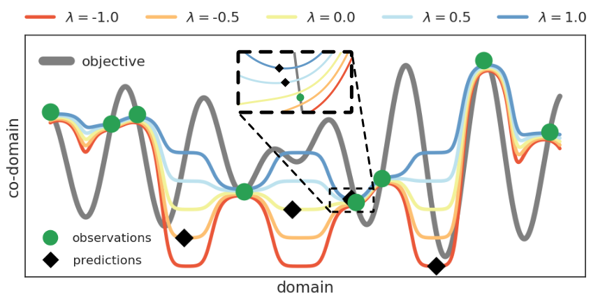
With a large positive value for , PHOENICS favors exploitation, while a large negative value favors exploration. When , the acquisition function approximates the objective function itself. Fig. 2 illustrates the behavior of PHOENICS on a one-dimensional objective function with different values. In this example, the acquisition function is constructed from eight observations indicated in green. Acquisition functions which were constructed from a more positive show low values only in the vicinity of the observation with the lowest objective function value. In contrast, acquisition functions which were constructed from a more negative show low values far away from any observation. The choice for the value of the exploration parameter can therefore be directly related to explorative or exploitative behavior.
From Fig. 2 we see that distinct points in parameter space are proposed based on particular values of the exploration parameter . The best choice of for a given objective function is a priori unknown. However, with the possibility to rapidly construct several acquisition functions with biases towards exploration or exploitation, we can propose multiple parameter points in batches based on different sampling strategies. The newly proposed parameter points are then evaluated on the black-box optimization function in possibly parallel evaluation runs.
III.3 Proxy optimization
New points in parameter space for querying the objective function are proposed based on the global minimum of the acquisition function (see Eq. 12, and Fig. 2). The problem of finding the global minimum of the objective function, which is costly to evaluate, is therefore reduced to searching the global minimum of the function approximation.
As a compromise of accuracy and computational cost, we search for the global minimum of the approximating function by uniformly sampling points in the parameter space and then running a gradient based optimizer on half of the proposed samples on the objective function approximation. Unless otherwise noted, all reported results were obtained from proposing uniform samples for each dimension of the parameter space and locally optimizing half of the sampled points with the L-BFGS algorithm for at most optimization steps.[40]
IV Results & Discussion
In this section we report the performance of PHOENICS and compare it to two frequently used global optimization packages built on Bayesian optimization. The “spearmint” software package performs Bayesian optimization using GPs and the predictive entropy acquisition function.[51, 52] The SMAC software employs RF models.[25, 26, 50]
The performance of each of these three optimization algorithms is evaluated on a set of 15 qualitatively different benchmark functions, which are continuous and convex, non-convex or discrete with possibly multiple local minima. Nine of the employed functions, which have a continuous co-domain, are well-established benchmarks for global optimization benchmarks. Additionally, we design six difficult cases with discrete co-domain. A complete list of the employed objective functions as well as their global minima is provided in the supplementary information (see Sec. VI.1).
We performed independent runs initialized with different random seeds, unless noted otherwise. During each optimization run we record the lowest achieved objective function value after each iteration. We compare the averaged lowest achieved objective function values by relating to results from simple random searches. Each random search was run for objective function evaluations and results were averaged over independent runs initialized with different random seeds. The average lowest achieved objective function values of the random search runs are summarized in the supplementary information (see Tab. 3).
IV.1 Two dimensional benchmarks
We start our discussion with a benchmark on the test functions mentioned above on two dimensional parameter spaces. PHOENICS was set up with three different values for the sampling parameter, , to assess the effectiveness of a particular parameter choice. Lowest objective function values achieved by each of the three considered optimization algorithms were recorded for independent runs initialized with a common set of random seeds.
In Fig. 3 we report the number of objective function evaluations required by each of the optimization algorithms to reach an objective function value lower than the average lowest value found in random searches within evaluations (see Tab. 3). Optimization traces for these runs on all 15 objective functions are reported in the supplementary information (see Sec. VI.4).

We find that GP optimization, as implemented in spearmint, generally quickly finds the global minimum if the objective function is strictly convex. In contrast, RF optimization, as implemented in SMAC, quickly finds the global minimum of objective functions with a discrete co-domain.
The performance of PHOENICS varies with different values of the sampling parameter . When favoring exploitation over exploration, i.e. the algorithm performs better if the objective function features narrow and well defined funnels (e.g. Ackley in Fig. 3a or Schwefel in Fig. 3c). With this choice for the sampling parameter, the algorithm is slightly biased towards exploring the local region around the current optimum. This behavior, however, is unfavorable in other cases, for instance when the objective function has a discrete co-domain (e.g. dAckley in Fig. 3d). Since parameter points in the vicinity to the current optimum likely yield the same value if the objective function is discrete or quasi-discrete, PHOENICS performs better on such objective functions when favoring exploration over exploitation, i.e. .
IV.2 Batch optimization
The dependence of the performance of PHOENICS on the sampling parameter could be eliminated by marginalizing over this parameter. Marginalization over the sampling parameter would effectively average out the advantageous effects of a bias towards exploitation for some objective functions and towards exploration for other objective functions.
The shape of the objective function is a priori unknown, so suitable choices of the sampling parameter cannot be determined beforehand, hence marginalization appears to be a solution. However, since the sampling parameter can be directly related to the explorative and exploitative behavior of the algorithm (see Sec. III.2) we continue with investigating a different approach to take full advantage of the sampling policy. We suggest to propose new parameter points based on a number of different sampling parameter values to keep the advantages of favored exploration and favored exploitation.
Given a set of observations the construction of several approximations to the objective function with different values of is computationally cheap. We can therefore easily suggest multiple new parameter points in batches at each optimization iteration, which are proposed from more explorative and more exploitative parameter values, at almost no additional cost. With the observations on the simple benchmarks in Sec. IV.1 we would expect a synergistic effect of this batch optimization over sequential optimization with a single sampling parameter value. As parameter points can be proposed with both a bias towards exploration and a bias towards exploitation, we expect the number of required objective function evaluations for reaching the global optimum to decrease. In addition, suggesting a batch of parameter points in one optimization step allows for the parallel evaluation of all proposed points, which accelerates the optimization process.
We demonstrate the aforementioned synergistic effect by running the optimization algorithm on the previously studied objective functions (see Fig. 3) with a different number of parameter points proposed per batch. Both, spearmint and SMAC allow for a parallel evaluation of a given objective function. With the spearmint package, multiple samples are generated by marginalizing over the possible outcomes of currently running experiments. The SMAC package allows for parallel objective function evaluations by running multiple regressor instances, which share a common set of objective function evaluations.
Tab. 1 summarizes the results for a simple batch optimization experiment on a selected set of objective functions. We again report the number of evaluations needed by each optimizer to reach an objective function value lower than the lowest average value found in random search with iterations. PHOENICS was run with sampling parameter values evenly spread out over the interval. Note, that the evaluation of a batch with samples was counted as evaluations of the objective functions. Traces of the lowest achieved objective function values are also depicted in the supplementary information (see Sec. VI.5).
| Method | Ackley | Dejong | Schwefel | dAckley | |
|---|---|---|---|---|---|
| PHOENICS | |||||
| RF | |||||
| GP | |||||
The behavior of the three studied optimization algorithms under parallel optimization on the Ackley objective function is illustrated in Fig. 4. In this figure we depict the minimum achieved objective function values for different runs with a different number of parallel evaluations of the objective function averaged over independent runs. The minimum achieved objective function values are presented per number of objective function evaluations (left panel) and per batch evaluation (right panel).

We find that both spearmint and SMAC achieve low objective function values in fewer batches with an increasing number of points proposed in each batch. While increasing the number of samples proposed per batch initially significantly improves the performance with respect to the number of proposed batches, this advantageous effect quickly levels off until there is no significant improvement beyond six samples per batch. However, when comparing the minimum achieved objective function values with respect to the total number of objective function evaluations, we did not observe any significant difference between runs with a different number of samples proposed per batch.
In contrast, PHOENICS shows a different behavior. Our algorithm does not only reach lower objective function values in a fewer number of batches when proposing more samples per batch, but also shows a better performance when considering the total number of function evaluations. This synergistic effect demonstrates that PHOENICS indeed benefits from proposing points in batches even in cases in which proposed samples are evaluated sequentially.
The performance improvement of PHOENICS when proposing parameter points in batches at each optimization iteration is demonstrated on all 15 considered objective functions in the supplementary information (see Sec. VI.5). We ran our optimizer with four points per batch, which are proposed from sampling parameter values evenly spaced across the interval. All four proposed parameter points are then evaluated before we started another optimization iteration. For this particular batching protocol, we find that PHOENICS outperforms RF based optimization on all benchmark functions and GP based optimization on 12 out of 15 benchmark functions. If and only if the objective function is convex, GP optimization finds lower objective function values. In addition, we observe the aforementioned synergistic effect of batch optimization for 12 out of 15 benchmark functions. Despite reducing the number of optimization iterations by a factor of 4, the achieved objective function values were found to be lower than values achieved in sequential optimizations with all three considered fixed sample parameter value.
We suggest that this improved performance of the algorithm is due to the trade-off between exploration and exploitation: while some of the samples proposed in one batch were suggested from parameter values which favor exploration, others are proposed for exploitation and locally exploring the region close to the currently lowest discovered objective function value. The exploration samples therefore systematically sample the parameter space and ensure that the algorithm does not get stuck in local minima, while the exploitation samples explore the local environment of the current global minimum. This sampling behavior is illustrated in Fig. 5 for the Michalewicz function.

The optimization runs on the Michalewicz function depicted in Fig. 5 were all started from the same two random samples illustrated in black for all three investigated optimization algorithms. Bayesian optimization based on GPs as implemented in spearmint (lower panels) tends to sample many parameter points close to the boundaries of the domain space in this particular example. RF optimization as implemented in SMAC (central panels), however, shows a higher tendency of exploring the parameter space.
PHOENICS (upper panels) starts exploring the space and quickly finds a local minimum in vicinity of one of the initial samples. After finding this local minimum, samples which are proposed based on a more exploitative (positive) value of the sampling parameter explore the local environment of this local minimum while samples proposed from more explorative (negative) values of explore the entire parameter space. As soon as the exploration points find a point in parameter space with a lower value of the objective function, the exploitation points jump to this new region in parameter space and locally explore the region around the current best to quickly converge to the global minimum.
Overall we have demonstrated that the value of the sampling parameter in the proposed acquisition function clearly influences the behavior of the optimization procedure towards a more explorative behavior for more negative values of this parameter and a more exploitative behavior for more positive parameter values. Batched optimization improves the performance of PHOENICS even in terms of total objective function evaluations and reduces the number of required optimization iterations.
IV.3 Increasing the number of dimensions
Real-life chemical problems are frequently concerned with more than just two parameters. Chemical reactions can be influenced by environmental conditions and experimental device settings, and computational studies frequently employ parameters to describe the system of interest. As such, this section focuses on the performance of PHOENICS in parameter spaces with dimensions .
When moving towards higher dimensional spaces, the chance for a uniformly sampled point to be close to the boundaries of the considered -dimensional hypercube increases, i.e. most sampled points will be close to the edges. Likewise, the volume of the region close to the global optimum decreases with respect to the total volume of the hypercube. Thus, we expect PHOENICS , RF and GP to perform worse for higher dimensional spaces.
We evaluated the performance of the three considered optimization algorithms on the subset of objective functions already considered in Sec. IV.1, but now successively increase the dimensionality of the parameter space from two to . Based on the results on batch optimization (see Sec. IV.2) we ran GP optimization and RF optimization with one point per batch and the optimization algorithm introduced in this study with four points per batch on each considered benchmark function. Exploration parameter values were chosen to be evenly spaced across the interval.
For better comparisons we report the average deviation of the lowest encountered objective function value from the global minimum of each function taken over independent optimization runs. Average deviations achieved by each of the optimization algorithms after objective function evaluations are depicted in Fig. 6.

We observe that PHOENICS maintains its rapid optimization properties for a variety of different objective functions even when increasing the number of dimensions. In the case of the Ackley function (Fig. 6a) PHOENICS appears to find and explore the major funnel close to the global optimum faster than the other two optimization algorithms regardless of the number of dimensions. The paraboloid (Fig. 6b) is an easy case for the GP in low dimensions, but is optimized the fastest by PHOENICS when considering parameter spaces with seven or more dimensions. No major differences are observed for the Schwefel function (Fig. 6c). However, in the case of a discrete objective function (Fig. 6d) PHOENICS seems to have a slight advantage over the other two optimizers for lower dimensions and performs about as well as random forest optimization for higher dimensions.
V Applications to chemistry
PHOENICS was shown to rapidly find the global optima of analytic objective functions used for benchmarking global optimization algorithms (see Sec. IV). In this section, we demonstrate its performance on the Oregonator, a model system of a chemical reaction described by a set of non-linear coupled differential equations.[16]
Most chemical reactions lead to a steady-state, i.e. a state in which the concentrations of involved compounds are constant in time. While chemical reactions described by a single differential equation always feature such a steady-state, more complicated dynamics phenomena can arise for reactions described by sets of nonlinear coupled differential equations. With the right choice of parameters, such differential equations may have a stable limit cycle, leading to periodic oscillations in the concentrations of involved compounds.[29, 62] With other parameter choices, however, the same chemical system might feature an attractive fixed point instead.
One of the earliest discovered reactions featuring a stable limit cycle for a set of reaction conditions is the Belousov-Zhabotinsky reaction.[11, 61] This network of chemical reactions involves temporal oscillations of [Ce] and [Ce]. The entire reaction network can be written as a set of three subreactions listed in Reaction VI.7. For details on the mechanism we refer to a brief summary in the supplementary information (see Sec. VI.7) as well as to the literature.[61, 14, 16, 20, 15]
Models at different levels of complexity have been developed to describe the dynamic behavior of the Belousov-Zhabotinsky reaction.[15, 2, 29, 57] One of the simplest models of this reaction is the Oregonator.[16] The Oregonator consists of a set of three coupled first order non-linear differential equations for three model compounds , and , which are shown in Eqs. 13 to 15. These equations involve five reaction constants , a stoichiometric factor , determined by the prevalence of one subreaction over another subreaction, and the concentration of two additional chemical compounds and . A map of Eqs. 13 to 15 to Reaction VI.7 is outlined in Ref. [16]
| (13) | ||||
| (14) | ||||
| (15) |
The set of differential equations in the Oregonator can be reduced into a dimensionless form, such that the number of correlated parameters is reduced to a smaller set of independent parameters. This reduced version of the Oregonator, shown in Eqs. V to V, includes three dimensionless variables , and , which describe the concentration of chemical species, and four dimensionless reaction constants , , and .
PHOENICSisusedtoreverseengineerthesetofreactionparametersconsistingofthreeinitialconditionsandfourreactionconstantsfromtheconcentrationtracescomputedintheoriginalpublication.[16]Thegoalistwofold:(i)findasetofparametersforwhichthedynamicalbehaviorqualitativelyagreeswiththebehaviorofthetarget,i.e.findchemicaloscillationsand(ii)finetunethissetofparameterssuchthatwereproducethedynamicalbehavioronaquantitativeleveltoaccuratelypredicttheconcentrationtracesfortheinvolvedcompounds.
Weimplementedafourth-orderRungeKuttaintegratorwithadaptivetimesteppingtocomputetheconcentrationtracesforagivensetofreactionparameters.Foreachproposedsetweusethisintegratortoevolvethedifferentialequationsandobtainconcentrationsonaregulargridviacubicsplineinterpolation.Theintegratorwasrunforatotalof10^712100λ[-1, 1]5015030050010050150
VI Conclusion
In this work we introduced PHOENICS, a novel algorithm for the global optimization of expensive to evaluate black-box objective functions. Our probabilistic optimizer combines Bayesian optimization with conceptual aspects of Bayesian Kernel Density estimation. Through an exhaustive benchmark study, we showed that PHOENICS improves over existing global optimization methods.
We formulate an inexpensive acquisition function balancing the explorative and exploitative behavior of the algorithm. This acquisition function enables intuitive sampling policies for an efficient parallel search of global minima. By leveraging synergistic effects from running multiple sampling policies in batches, the performance of the algorithm improves, and requires a reduced total number of objective function evaluations.
Benchmark results were compared to popular Bayesian optimization methods based on GPs and RFs. Unlike GP and RF, PHOENICS appears to be less sensitive to the nature of the co-domain. Notably, PHOENICS was shown to outperform RF in all 15 test functions, and to outperform GP in all 12 non-convex test functions. When moving towards higher dimensional spaces, we observed that PHOENICS maintains its rapid optimization properties for a variety of different objective functions.
We illustrated the capabilities of our algorithm for an inverse design problem on the Oregonator, a practical example for a model system describing a complex chemical reaction network. We demonstrated that only PHOENICS was able to reproduce the qualitative and quantitative target dynamic behavior of the nonlinear reaction dynamics.
We believe that PHOENICS has the potential to be applied to a wide range of applications, from optimization of reaction conditions and material properties, over control of robotics systems, to circuit design for quantum computing.[45, 47]
All in all, we recommend PHOENICS for an efficient optimization of scalar, possibly non-convex, black-box unknown objective functions.
Acknowledgments
We thank Dr. S. K. Saikin for fruitful discussions and helpful comments. F.H. was supported by the Herchel Smith Graduate Fellowship. L.M.R and A.A.G were supported by the Tata Sons Limited - Alliance Agreement (A32391). C.K. and A.A.G were supported by the National Science Foundation under award number CHE-1464862. All computations reported in this paper were completed on the Odyssey cluster supported by the FAS Division of Science, Research Computing Group at Harvard University.
References
- [1] R. A. Fisher. The design of experiments. Oliver and Boyd; Edinburgh; London, 1937.
- [2] G. E. P. Box, J. S. Hunter, and W. G. Hunter. Statistics for experimenters: design, innovation and discovery, volume 2. 2005.
- [3] M. J. Anderson and P. J. Whitcomb. DOE simplified: pratical tools for effective experimentation. CRC Press, 2016.
- [4] D. M. Negoescu, P. I. Frazier, and W. B. Powell. The knowledge-gradient algorithm for sequencing experiments in drug discovery. INFORMS Journal on Computing, 23(3):346–363, 2011.
- [5] S. A. Lopez, B. Sanchez-Lengeling, J. de Goes Soares, and A. Aspuru-Guzik. Design principles and top non-fullerence acceptor candidates for organic photovoltaics. Joule, 2017.
- [6] J. N. Wei, D. Duvenaud, and A. Aspuru-Guzik. Neural networks for the prediction of organic chemistry reactions. ACS Cent. Sci., 2:725–732, 2016.
- [7] C. W. Coley, R. Barzilay, T. S. Jaakkola, W. H. Green, and K. F. Jensen. Prediction of organic reaction outcomes using machine learning. ACS Cent. Sci., 3:434–443, 2017.
- [8] M. H. S. Segler and M. P. Waller. Neural-symbolic machine learning for retrosynthesis and reaction prediction. Chemistry-A European Journal, 23:5966–5971, 2017.
- [9] D. J. Lizotte, T. Wang, M. H. Bowling, and D. Schuurmans. Automatic gait optimization with gaussian process regression. In IJCAI, volume 7, pages 944–949, 2007.
- [10] P. Nikolaev, D. Hooper, N. Perea-Lopez, M. Terrones, and B. Maruyama. Discover of wall-selective carbon nanotube growth conditions via automated experimentation. ACS nano, 8(10):10214–10222, 2014.
- [11] Pavel Nikolaev, Daylond Hooper, Frederick Webber, Rahul Rao, Kevin Decker, Michael Krein, Jason Poleski, Rick Barto, and Benji Maruyama. Autonomy in materials research: a case study in carbon nanotube growth. npj Computational Materials, 2:16031, 2016.
- [12] L. Cronin, V. Duros, J. Grizou, W. Xuan, Z. Hosni, D. L. Long, and H. Miras. Human vs robots in the discovery and crystallization of gigantic polyoxometalates. Angew. Chem. Int. Ed., 56:10815–10820, 2017.
- [13] J. A. Bergstra, R. Badenet, Y. Bengio, and B. Kégl. Algorithms for hyper-parameter optimization. In Advances in Neural Information Processing Systems, pages 2546–2554, 2011.
- [14] J. Bergstra and Y. Bengio. Random search for hyper-parameter optimization. J. Mach. Learn. Res., 13:281–305, 2012.
- [15] H. J. Kushner. A new method of locating the maximum point of an arbitrary multipeak curve in the presence of noise. J. Basic. Eng., 86(1):97–106, 1964.
- [16] J. Močkus. On bayesian methods for seeking the extremum. In Optimization Techniques IFIP Technical Conference, pages 400–404, 1975.
- [17] J. Močkus. The bayesian approach to global optimization. System Modeling and Optimization, pages 473–481, 1982.
- [18] J. Snoek, H. Larochelle, and R. P. Adams. Practical bayesian optimization of machine learning algorithms. In Advances in Neural Information Processing Systems, volume 25, pages 2951–2959. 2012.
- [19] N. Scrivinas, A. Krause, S. M. Kakade, and M. W. Seeger. Information-theoretic regret bounds for gaussian process optimization in the bandit setting. IEEE Transactions on Information Theory, 58:3250–3265, 2012.
- [20] M. Lindauer, K. Eggensperger, M. Feurer, S. Falkner, A. Biedenkapp, and F. Hutter. Smac v3: Algorithm configuration in python. https://github.com/automl/SMAC3, 2017.
- [21] F. Hutter, H. Hoos, and K. Leyton-Brown. Sequential model-based optimization for general algorithmic configuration. volume 5. 2011.
- [22] F. Hutter, H. Hoos, and K. Leyton-Brown. Parallel algorithm configuration. Learning and Intelligent Optimization, pages 55–70, 2012.
- [23] J. Snoek, K. Swersky, R. Zemel, and R. P. Adams. Input warping for bayesian optimization of non-stationary functions. In International Conference on Machine Learning, pages 1674–1682, 2014.
- [24] J. Snoek, O. Rippel, K. Swersky, R. Kiros, N. Satish, N. Sundaram, M. Patwary, Prabhat, and R. Adams. Scalable bayesian optimization using deep neural networks. In Proceedigns of the 32nd International Conference on Machine Learning, volume 37, pages 2171–2180, 2015.
- [25] J. R. Springenberg, A. Klein, S. Falkner, and F. Hutter. Bayesian optimization with robust bayesian neural networks. In Advances in Neural Information Processing Systems, pages 4134–4142, 2016.
- [26] D. R. Jones, M. Schonlau, and W. J. Welch. Efficient global optimization of expensive black-box functions. J. Glob. Opt., 13(4):455–492, 1998.
- [27] J. M. Hernández-Lobato, M. Gelbart, M. Hoffman, R. P. Adams, and Z. Ghahramani. Predictive entropy search for efficient global optimization of black-box functions. In Advances in neural information processing systems, pages 918–926, 2014.
- [28] J. M. Hernández-Lobato, M. Gelbart, M. Hoffman, R. P. Adams, and Z. Ghahramani. Predictive entropy search for bayesian optimziation with unknown constraints. In Proceedings of the 32nd International Conference on Machine Learning, volume 37, pages 1699–1707, 2015.
- [29] N. Srivinas, A. Krause, M. Seeger, and S. M. Kakade. Gaussian process optimization in the bandit setting: No regret and experimental design. In Proceedings of the 27th International Conference on Machine Learning (ICML), pages 1015–1022, 2010.
- [30] R. Gómez-Bombarelli, D. Duvenaud, J. M. Hernández-Lobato, J. Aguilera-Iparraguirre, R. D. Hirzel, R. P. Adams, and A. Aspuru-Guzik. Automatic chemical design using a data-driven continuous representation of molecules. arXiv preprint arXiv:1610.02415, 2016.
- [31] Edward O Pyzer-Knapp, Gregor N Simm, and Alán Aspuru Guzik. A bayesian approach to calibrating high-throughput virtual screening results and application to organic photovoltaic materials. Materials Horizons, 3(3):226–233, 2016.
- [32] F. Häse, C. Kreisbeck, and A. Aspuru-Guzik. Machine learnig for quantum dynamics: deep learning of excitation energy transfer properties. Chem. Sci., 8:8419–8426, 2017.
- [33] Ruben Martinez-Cantin. Bayesian optimization with adaptive kernels for robot control. In Robotics and Automation (ICRA), 2017 IEEE International Conference on, pages 3350–3356. IEEE, 2017.
- [34] Shenghong Ju, Takuma Shiga, Lei Feng, Zhufeng Hou, Koji Tsuda, and Junichiro Shiomi. Designing nanostructures for phonon transport via bayesian optimization. Physical Review X, 7(2):021024, 2017.
- [35] L Cornejo-Bueno, EC Garrido-Merchán, D Hernández-Lobato, and S Salcedo-Sanz. Bayesian optimization of a hybrid system for robust ocean wave features prediction. Neurocomputing, 2017.
- [36] Shun Kikuchi, Hiromi Oda, Shin Kiyohara, and Teruyasu Mizoguchi. Bayesian optimization for efficient determination of metal oxide grain boundary structures. Physica B: Condensed Matter, 2017.
- [37] Z. Wang, C. Li, S. Jegelka, and P. Kohli. Batched high-dimensional bayesian optimization via structural kernel learning. arXiv preprint arXiv:1703.01973, 2017.
- [38] E. Contal, D. Buffoni, A. Robicquet, and N. Vayatis. Parallel gaussian process optimization with upper confidence bound and pure exploration. In Joint European Conference on Machine Learning with Knowledge Discovery in Databases, pages 225–240, 2013.
- [39] T. Desautels, A. Krause, and J. W. Burdick. Parallelizing exploration-exploitation tradeoffs in gaussian process bandit optimization. J. Mach. Learn. Res., 15(1):3873–3923, 2014.
- [40] F. Häse, L. M. Roch, C. Kreisbeck, and A. Aspuru-Guzik. Phoenics: A universal deep bayesian optimizer (https://github.com/florianhase/phoenics). GitHub, 2017.
- [41] M. A. Osborne, R. Garnett, and S. J. Roberts. Gaussian processes for global optimization. In 3rd international conference on learning and intelligent optimization (LION3), pages 1–15, 2009.
- [42] R. Martinez-Cantin, N. de Freitas, E. Brochu, J. Castellanor, and A. Doucet. A bayesian exporation-exploitation approach for optimal online sensing and planning with a visually guided mobile robot. Autonomous Robots, 27:29–103, 2009.
- [43] L. Breiman. Random forests. Machine learning, 45:5–32, 2001.
- [44] C. K. I. Williams. Computing with infinite networks. In Advances in neural information processing systems, pages 295–301, 1997.
- [45] T. Kathuria, A. Deshpande, and P. Kohli. Batched gaussian process bandit optimization via determinantal point processes. In Advances in Neural Information Processing Systems, pages 4206–4214, 2016.
- [46] Michael D Escobar and Mike West. Bayesian density estimation and inference using mixtures. J. Am. Stat. Assoc., 90(430):577–588, 1995.
- [47] M. D. Hoffman and A. Gelman. The no-u-turn sampler: adaptively setting path lengths in hamiltonian monte carlo. J. Mach. Learn. Res., 15:1593–1623, 2014.
- [48] J. Salvatier, T. V. Wiecki, and C. Fonnesbeck. Probabilistic programming in python using pymc3. PeerJ Comp. Sci., 2:e55, 2016.
- [49] José Luis Morales and Jorge Nocedal. Remark on “algorithm 778: L-bfgs-b: Fortran subroutines for large-scale bound constrained optimization”. ACM Transactions on Mathematical Software (TOMS), 38(1):7, 2011.
- [50] R. J. Field and R. M. Noyes. Oscillations in chemical systems. iv. limit cycle behavior in a model of a real chemical reaction. J. Chem. Phys., 60(5):1877–1884, 1974.
- [51] N. G. Van Kampen. Stochastic processes in physics and chemistry, volume 1. 1992.
- [52] A. M. Zhabotinsky. A history of chemical oscillations and waves. Chaos, 1:379–386, 1991.
- [53] H. Deng. Effect of bromine derivatives of malonic acid on the oscillating reaction of malonic acid, cerium ions and bromate. Nature, 213:589–590, 1967.
- [54] A. M. Zhabotisnky and A. N. Zaikin. Oscillatory processes in biological and chemical systems. Izdatelstro ”Nauka” Publishers, Moscow, 1967.
- [55] R. J. Field, E. Koros, and R. M. Boyes. Oscillations in chemical systems. ii. thorough analysis of temporal oscillation in the bromate-cerium-malonic acid system. J. Am. Chem. Soc., 94:8649–8664, 1972.
- [56] L. Gyorgyi, R. Turányi, and R. J. Field. Mechanistic details of the oscillatory belousov-zhabotinski reaction. J. Phys. Chem., 94:7162–7170, 1990.
- [57] R. J. Field. Das experiment: Eine oszillierende reaktion. Chemie in unserer Zeit, 7:171–176, 1973.
- [58] K. Bar-Eli. The minimal bormate oscillator simplified. J. Phys. Chem., 89:2855–2860, 1985.
- [59] V. Voorsluijs, I. G. Kevrekidis, and Y. De Decker. Nonlinear behavior and fluctuation-induced dynamics in the photosensitive belousov–zhabotinsky reaction. Phys. Chem. Chem. Phys., 19:22528–22537, 2017.
- [60] L. Kuhnert. Selbstorganisation chemischer Strukturen: Arbeiten von Friedlieb Ferdinand Runge, Raphael Eduard Liesegang, Boris Pavlovich Belousov u. Anatol Markovich Zhabotinsky. 1987.
- [61] A. Peruzzo, J. McClean, P. Shadbolt, M. H. Yung, X. Q. Zhou, P. J. Love, A. Aspuru-Guzik, and J. L. O’brien. A variational eigenvalue solver on a photonic quantum processor. Nature comm., 5, 2014.
- [62] J. Romero, J. P. Olson, and A. Aspuru-Guzik. Quantum autoencoders for efficient compression of quantum data. Quantum Science and Technology, 2(4):045001, 2017.
Supplementary information
VI.1 Analytic objective functions
We benchmarked the performance of the global optimization algorithm PHOENICS on a total of 15 analytic objective functions. Nine of these objective functions have a continuous co-domain and are commonly used to benchmark algorithms developed for unconstrained optimization problems. The remaining six benchmark functions have a discrete co-domain and were specifically designed for this study. We provide Python implementations for all 15 benchmark functions on a GitHub repository.[18]
The nine analytic benchmark functions with continuous co-domain were chosen based on their different features: they differ in the number of local minima, number of global minima and the dimensionality of the parameter space for which they are defined. Details are summarized in Tab. 2. Fig. 9 displays contour plots of all objective functions for a two dimensional parameter space.
All of the benchmark functions with discrete co-domain project the parameter space onto integer values in the interval. Contour plots for these benchmark functions are displayed in Fig. 9 for a two dimensional parameter space, although all of the six functions generalize to higher dimensions as well. Note, that the global minimum of these functions is not a unique point in parameter space, but rather an entire region.

| Objective function | Domain range | Global minimum (2d) | generalizable |
|---|---|---|---|
| Ackley | yes | ||
| Branin | no | ||
| Camel | no | ||
| Dejong | yes | ||
| Ellipsoid | yes | ||
| Michalewicz | no | ||
| Rastrigin | yes | ||
| Rosenbrock | yes | ||
| Schwefel | yes |
VI.2 Random search results
The employed analytic benchmark functions (see Sec. VI.1) differ drastically in their shape. While some functions, like the Ackley function or the Schwefel function feature narrow local funnels around their global minima, other functions such as Branin and Dejong have rather broad funnels. The benchmark functions also differ greatly in the range of their co-domain spaces. Instead of reporting the deviation of the current best to the global minimum during an optimization run we therefore compare the optimization algorithms to random searches on the same objective functions.
In one random search run we evaluated each objective function times at positions uniformly sampled from the domain space. The lowest achieved function value averaged over random searches with different random seeds serves as the benchmark value for each optimization algorithm. For each algorithm, we record the number of function evaluations needed to discover a point in parameter space which yields a function value lower than the average lowest value encountered in the random searches. The average lowest values for all objective functions in two dimensions are summarized in Tab. 3.
| Loss function | Global minimum | Lowest encounter |
|---|---|---|
| Ackley | ||
| Branin | ||
| Camel | ||
| Dejong | ||
| Ellipsoid | ||
| Michalewicz | ||
| Rastrigin | ||
| Rosenbrock | ||
| Schwefel |
| Loss function | Global minimum | Lowest encounter |
|---|---|---|
| Linear funnel | ||
| Narrow funnel | ||
| Double well | ||
| Disc. Ackley | ||
| Disc. Michalewicz | ||
| Disc. Valleys |
VI.3 Precision
In this work we propose to approximate a given objective function with a prior constructed from Gaussian distributions. Given a set of observations of pairs of parameter points and corresponding objective function values, the approximation to the objective function is constructed from Gaussians. The locations of the Gaussian distributions are drawn from a BNN trained to predict the locations of observed parameter points. Precisions of these Gaussians, however, are drawn from a Gamma distribution parametrized via a probability density function as presented in Eq. 43, where denotes the Gamma function.
| (43) |
The prior for this Gamma distribution is chosen to be and for a given set of observations. With this choice of hyperparameters the expectation value for the prediction is . The prefactor in the expectation value of the precision ensures that in the case of only a single observation the standard deviation of the approximating Gaussian distribution matches the standard deviation of a uniform distribution along a single dimension of the unit hypercube. Starting out from an uninformative uniform prior we therefore gradually increase our believe about the parameter space with this particular choice of the prefactor. The dependence of the hyperparameter on the number of observations guarantees that the precision of the Gaussian distributions increases with more observations, i.e. the standard deviation of the Gaussian decreases. This decrease in the standard deviation with the number of observations is necessary for the convergence of the approximative model to the objective function in the limit of an infinite number of observations.
Several different protocols could be applied to increase the precision of the Gaussian distributions with the number of observations. In a scenario in which a dataset consisting of observations is approximated by a single Gaussian distribution, the precision of the Gaussian increases as the square root of the number of observed points, i.e. . Likewise we can consider a case in which we sample a random variable from the sum of Gaussian distributions. Assuming each of the Gaussian distributions has the same standard deviation , the standard deviation of the random variable is given by .
Based on these two considerations we studied the performance of PHOENICS with three different protocols for increasing the precision of the Gaussians with the number of observations: increasing the expected value of the precision with the number of observations as (i) , (ii) and (iii) given on the prior considerations. Results of the benchmark runs with PHOENICS and the three different schedules on selected objective functions are reported in Tab. 4. We report the minimum number of required objective function evaluations to reach values lower than the average lowest value encountered after random evaluations of the objective function (see Sec. VI.2).
| Protocol | Ackley | Dejong | Schwefel | dAckley |
|---|---|---|---|---|
We find, that the schedule for shrinking approximating Gaussian distributions performs the best out of the proposed shrinking schedules across all objective functions. Slower increases in the precision of the Gaussian distributions like in the schedule seem to create persistent regions in parameter space for which the acquisition function predicts unfavorable objective function values and does not sufficiently enhance exploration. In contrast, the schedule shrinks Gaussian distributions too quickly such that acquired knowledge cannot be exploited sufficiently and the algorithm behaves more like random search. Based on these findings, PHOENICS adopts the as shrinking schedule.
VI.4 Benchmark results
We benchmarked PHOENICS, RF and GP optimizers on a total of 15 different benchmark functions, which are reported and discussed in detail in Sec. VI.1. For each of the benchmark function we ran the optimization algorithm for a total of iterations in independent runs initialized with different random seeds and recorded the lowest discovered objective function values for each iteration. Each objective function was optimized by three independent optimizer instances constructed from different exploration parameter values .
Average lowest discovered objective function values and bootstrapped uncertainties are depicted in Fig. 10. For comparison we provide the average lowest objective function values discovered by Bayesian optimization with Gaussian processes as implemented in spearmint and with random forests as implemented in SMAC.

We find that instances of the optimization algorithm introduced in this study perform better than GP optimization and RF optimization in eleven out of 15 cases. For all studied objective function, instances of the introduced optimization algorithm perform better than RF optimization. GP optimization, however, discovers lower objective function values than instances of PHOENICS in four cases.
These four cases, for which GP optimization discovers lower objective function values, are cases of purely convex objective functions (Dejong, Ellipsoid and Rosenbrock) and the Rastrigin function, which is mostly convex with small local minima modulating a general hyperparabolic shape.
We further observe that for some objective functions a more explorative (more negative) value of the exploration parameter improves the performance while in other cases a more exploitative (more positive) value is beneficial. For instance in the case of objective functions with a discrete co-domain (right and second to right columns in Fig. 10) we observe good performance with more negative exploration parameter values. In fact, positive values for the exploration parameter result in the algorithm no longer finding the global minimum. This, however, can be explained by the fact that parameter points proposed with favoring exploitation will always be in close proximity to the current best observed parameter point. On a discrete co-domain, however, all points in close proximity to the current best yield the same objective function value.
In other cases, especially for mostly convex objective functions such as the Dejong function or the Camel function, PHOENICS performs the best when favoring exploitation over exploration. We therefore conclude that there cannot be a single best balance between exploration and exploitation for objective functions as diverse as the objective functions in this benchmark set.
VI.5 Batch optimization results
Instead of marginalizing over the exploration parameter in the acquisition function of PHOENICS , we suggest to propose parameter points in batches, some of which are determined favoring exploration and others favoring exploitation. Here, we demonstrate the the proposed algorithm benefits from such a procedure even if the proposed parameter points are evaluated sequentially.
Fig. 11 displays the lowest achieved deviations between sampled objective function values and their global minima for a selected set of objective functions. Results reported for each objective function are averaged over independent runs. PHOENICS was run by proposing parameter points in batches of points, which where then evaluated sequentially. The evaluation of points in one batch was counted as objective function evaluations. We report the number of objective function evaluations needed to reach the indicated objective function values. Values for the exploration parameter were drawn evenly spaced from the interval. We provide the lowest achieved objective functions values in GP optimization and RF optimization for comparison.

We observe that the synergistic effect of proposing parameter points in batches reported on the Ackley function in the main text (see Sec. 4) also occurs for the other studied objective functions. In fact, even for objective functions with a discrete co-domain (right panel, Fig. 11) batch optimization seems to enhance the performance of PHOENICS, although we demonstrated that PHOENICS does not perform well on objective functions with a discrete co-domain when proposing parameter points with a bias towards exploitation.
VI.6 Algorithm comparisons
We demonstrated that PHOENICS generally performs better when proposing parameter points in batches, where some of the parameter points are proposed with a bias towards exploration and others are proposed with a bias towards exploitation (see Sec. IV.2). Here, we report on the performance of PHOENICS with batch exploration and compare to RF and GP optimization. Fig. 12 depicts the traces of average deviations between the lowest achieved objective function values and their global minima for a total of independent runs with all three optimization algorithms. PHOENICS proposed points per batch based on exploration parameter values evenly spread across the interval.

We find that PHOENICS finds parameter points yielding objective function values closer to their global optima than RF and GP optimization in 12 out of 15 cases (indicated with in Fig. 12). PHOENICS is only outperformed by GP optimization if the objective function is convex, i.e. for the Dejong, Ellipsoid and Rosenbrock function. Nevertheless, PHOENICS finds reasonable parameter points yielding low objective function values even for these functions.
In addition, we observe a synergistic effect of batch optimization for 12 out of 15 objective functions (indicated with in Fig. 12). For these objective functions, batch optimization performs better than any of the exploration parameter choices reported in Fig. 10). We note, that the same batching protocol was used for all objective functions, indicating the flexibility and broad applicability of this protocol.
VI.7 Belousov-Zhabotinsky reaction mechanism
The Belousov-Zhabotinsky reaction is a prominent example of a nonlinear chemical oscillator.[61, 11] While the detailed reaction mechanism is rather complex and involved a large number of elementary subreactions,[20] the reaction can be summarized in three major subprocesses (see reaction VI.7).