Stellar parameters for the central star of the planetary nebula PRTM 1 using the German Astrophysical Virtual Observatory service TheoSSA

For precise spectral analysis of hot stars, observations with good quality and stellar-atmosphere models that account for reliable physics and deviations from the assumption of a local thermodynamic equilibrium (LTE) are necessary. Figure 1 illustrates that for cool stars with high surface gravity (spectral type B and later), LTE model atmospheres might be sufficient (Auer & Mihalas 1972, cf.,). There are, however, non-local thermodynamic equilibrium (NLTE) effects in any star, at least towards higher energies and in high-resolution spectra, particularly in the infrared (IR) wavelength range.

In the last century, NLTE model atmospheres were believed to be a domain of specialists, because they require high computational times and a lot of work on atomic data. Hence, the use of blackbody spectra to represent hot stars had been a common approximation in work where ionizing fluxes were required.

Several well documented NLTE codes were developed in that time (Hubeny & Mihalas 2014), e.g., the PHOENIX (Baron et al. 2010; Hauschildt & Baron 1999; Hauschildt & Baron 2010, http://www.hs.uni-hamburg.de/EN/For/ThA/phoenix), the TLUSTY (Hubeny & Lanz 2011; Hubeny 1988; Hubeny & Lanz 1992; Hubeny et al. 1994; Hubeny & Lanz 1995, http://nova.astro.umd.edu), and the TMAP (Werner et al. 2012, http://www.uni-tuebingen.de/de/41621,) code. The latter two are widely used, e.g., in spectral analyses of hot, compact stars. TMAP was successfully used for sdO/B stars (Rauch et al. 1991; Rauch 1993; Rauch et al. 2002; Rauch et al. 2010b; Klepp & Rauch 2011; Rauch et al. 2014, e.g.,), PG 1159-type stars (Werner et al. 1991; Jahn et al. 2007; Werner et al. 2015; Werner et al. 2016, e.g.,), DA-type white dwarfs (Werner & Rauch 1997; Rauch et al. 2013, e.g.,), DO-type white dwarfs (Hoyer et al. 2017; Rauch et al. 2017; Werner & Rauch 1997, e.g.,), central stars of planetary nebulae (Ercolano et al. 2003; Rauch et al. 2007; Ziegler et al. 2012, CSPN, e.g.,), super-soft X-ray sources (van Teeseling et al. 1999; Rauch et al. 2010b; Orio et al. 2013; Peretz et al. 2016, e.g.,), and neutron stars (Rauch et al. 2008, e.g.,).

In the framework of the Virtual Observatory (VO), the German Astrophysical Virtual Observatory (GAVO¹¹ 1 http://www.g-vo.org) project nowadays provides synthetic stellar spectra on demand via the registered Theoretical Stellar Spectra Access VO service (Rauch 2008; Rauch & Nickelt 2009; Rauch et al. 2009). TheoSSA is designed to host spectral energy distributions (SEDs) calculated by any model-atmosphere code. Initially, these SEDs should be used as realistic stellar ionizing fluxes for photoionization models of planetary nebulae (PNe). In addition, such SEDs can be used for spectral analyses (Rauch et al. 2010a; Ringat & Rauch 2010; Rauch & Ringat 2011; Ringat et al. 2012; Müller-Ringat 2013). The registered VO tool TMAW²² 2 http://astro.uni-tuebingen.de/~TMAW (Tübingen NLTE Model-Atmosphere WWW Interface) allows to calculate model atmospheres for hot, compact stars with the Tübingen NLTE model-atmosphere package (Rauch & Deetjen 2003; Werner et al. 2003, TMAP³³ 3 http://astro.uni-tuebingen.de/~TMAP), considering opacities of H, He, C, N, O, Ne, Na, and Mg (with individually user-chosen abundances). To represent these species, TMAW uses either standard or individually compiled model atoms based on data provided by the Tübingen Model Atom Database (TMAD⁴⁴ 4 http://astro.uni-tuebingen.de/~TMAD, cf., TMAP User’s Guide http://astro.uni-tuebingen.de/~TMAP/UserGuide/UserGuide.pdf). TMAW SEDs allow individual, detailed analyses and a more precise determination of effective temperature ($T_{\mathrm{eff}}$), surface gravity ($\log g$), and photospheric abundances of a star. Once calculated, the TMAW SEDs are automatically ingested by TheoSSA. Tables 2 and 3 show a TMAW request and the files that can be retrieved by the TMAW user after the end of the calculation, respectively.

The primary purpose of these SEDs was to perform preliminary spectral analyses and to achieve determinations of $T_{\mathrm{eff}}$, $\log g$, and abundances better than 20%. Rauch & Ringat (2012) and Ringat & Reindl (2013) demonstrated that the deviation of $T_{\mathrm{eff}}$ and $\log g$ values found with TMAW SEDs and with “manually calculated” TMAP models is of the order of 10%. To demonstrate a spectral analysis using TheoSSA and TMAW, we have chosen the hot central star (CS) of the planetary nebula PRTM 1 because no reliable determination of photospheric parameters like $T_{\mathrm{eff}}$, $\log g$, and element abundances is hitherto available.

Torres-Peimbert et al. (1990) discovered the very-high excitation PN PRTM 1 (PN G243.8$-$37.1), located in the Galactic halo at a distance of $d=5\pm 2\,\mathrm{kpc}$ and at a height below the Galactic plane of $|z|=3\pm 1.2\,\mathrm{kpc}$. Peña et al. (1990) found that, although carbon-poor, its heavy elements are not as underabundant as known from other halo PNe. In their PN analysis, they used a grid of SEDs from NLTE H+He models (Clegg & Middlemass 1987) and best reproduced the nebular ionization structure using an ionizing source with $T_{\mathrm{eff}}$ $\approx 90\,000\,\mathrm{K}$ and a surface gravity of $\log\,(g\,/\,\mathrm{cm/s^{2}})\approx 5.3$. This was in agreement with $\mbox{$T_{\mathrm{eff}}$}\hskip-1.42262pt=\hskip-1.42262pt90\,000\pm 10\,000\,\mathrm{K}$ determined by Feibelman (1998, from blackbody fits to the stellar continuum flux) and preliminary results of Méndez & Ruiz (priv. comm., mentioned by Peña et al. 1990, analysis method and error ranges unknown, based on optical observations) of $T_{\mathrm{eff}}\approx 80\,000\,\mathrm{K}$ and $\log g\approx 5.2$ that were then used to determine the stellar mass of $M=0.58\,M_{\odot}$. Peña et al. (1990) discovered a strong C deficiency of the order of 1 dex in the PN and suggested that the progenitor star was metal-poor with very low mass that did not undergo a third dredge up.

Méndez (1991) classified the CS of PN PRTM 1 as an O(H)-type star, i.e., its optical spectrum is dominated by hydrogen absorption lines. Stellar spectroscopic and photospheric variability was reported by Feibelman (1998, in the ultraviolet) and was confirmed by Peña & Ruiz (1998, in the optical with ≲ ⁢ Δ m V ⁢ 1 mag , = m V 16.6 in Oct 1990 and = m V ± 15.6 0.2 in Feb 1998).

Recently, the CS had been monitored during three months for its variability by Boffin et al. (2012), because its spectroscopic appearance matches that of the CSPN of Fleming 1 (Boffin et al. 2012, PN Fg 1, PN G290.5+07.9,) and thus, a binary nature was hypothesized. The obtained data, however, does not support this. The CS’s rectified average FORS2⁵⁵ 5 FOcal Reducer and low-dispersion Spectrograph spectrum (4597 Å – 5901 Å, slit width 0$\aas@@fstack{\prime\prime}$5, volume-phase holographic grating 1400V, resolution 1.22 Å full width at half maximum) taken at ESO’s VLT⁶⁶ 6 European Southern Observatory, Very Large Telescope is of good quality, suitable for a spectral analysis. It exhibits a variety of lines, namely of H i, He ii, C iv, N v, O v, and O vi. The latter two even allow to evaluate the O ionization equilibrium to determine $T_{\mathrm{eff}}$ precisely.

Since hitherto no spectral analysis appeared in the literature, we take the opportunity and use the average spectrum of this spectroscopically variable star to demonstrate how straightforward a NLTE spectral analysis became with the development of TheoSSA and TMAW. A time-dependent spectral analysis is desirable to further investigate on the nature of the star. This, however, is not the focus of this paper.

We start with a description of TheoSSA in Sect. 2. In Sect. 3, we briefly describe the coarse determination of $T_{\mathrm{eff}}$ and $\log g$ using pre-calculated synthetic H+He SEDs. A more individual analysis based on newly calculated stellar atmosphere models and SEDs is presented in Sect. 4. We summarize our results and conclude in Sect. 5.

TheoSSA is a spectral service fully integrated into the VO. This means that

1. 1.

   TheoSSA can easily be located using the VO Registry (Demleitner et al. 2015), a global inventory of services allowing the discovery of data services using a wide variety of constraints. Three example queries that would, among others, yield TheoSSA, are ‘‘all spectral services serving model spectra in the ultraviolet’’, ‘‘services dealing with white dwarfs’’, and ‘‘services created by Thomas Rauch’’. The metadata provided by the Registry also contains information on who to contact in case of technical problems or scientific questions, and what bibliographic sources to cite when using the data served. By virtue of being in the Registry, TheoSSA has a special URI⁷⁷ 7 unified resource identifier, the IVOID (Plante et al. 2007), that uniquely identifies it: ivo://org.gavo.dc/theossa/q/ssa.

2. 2.

   TheoSSA can be queried using a standard protocol called Simple Spectral Access (Tody et al. 2007, SSA,). This means that computer programs (“clients”) can use the same code to query TheoSSA and numerous other spectral services which are also discoverable through the VO Registry. Examples for such clients include Splat (Castro-Neves & Draper 2014) and VOSpec (Osuna et al. 2005), both containing functionality geared towards spectral analysis, as well as TOPCAT⁸⁸ 8 Tool for OPerations on Catalogues And Tables (Taylor 2005) for generic processing of tabular data (which includes spectra). For use without VO-enabled client software, TheoSSA also provides a conventional form-based interface for use with web browsers⁹⁹ 9 http://dc.g-vo.org/theossa.

3. 3.

   TheoSSA delivers spectra in standard formats, in particular in VOTables following the Spectral Data Model (McDowell et al. 2011). This lets clients not only immediately display spectra obtained from the service endpoint. The rich metadata also allows automatic unification of properties like units or spectral resolution between spectra obtained from different sources.

4. 4.

   TheoSSA offers an associate prototype service implementing the upcoming SODA (“Service Operations On Data”) standard. This allows on-the-fly, server-side format conversion and cutouts in the context of the general Datalink protocol, which itself is a generic way to link datasets with related artifacts (Dowler et al. 2015).

TheoSSA is operated at GAVO’s Heidelberg data center on top of the publicly available VO server package DaCHS (Demleitner et al. 2014).

SSA, the VO’s standard protocol for querying spectral services like TheoSSA, is in its core strongly biased towards observational data. Typical parameters used there include location of the aperture projected at the sky or the name of the target object. Though a few spectra in TheoSSA were computed assuming abundances of well-known objects (see below) and can be located by searching for these objects’ names, typically such parameters are not useful to constrain results from a “theory” service (in VO jargon, this denotes services publishing computed, rather than observed, data).

Instead, a service like TheoSSA employs numerous custom parameters, in particular w_<element> where <element> is an element name for the model abundances, t_eff for the model effective temperature, mdot for the mass loss rate, and log_g for the logarithm of the surface gravity (Figs. 9 and 10 display the TheoSSA TMAP Web Interface and its result page, respectively). All these float-valued parameters allow the specification of ranges using a slash; for instance log_g=5.5/7 will select all spectra with $5.5\leq\log g\leq 7$, with half-open variants like /7 or 5.5/ working as expected. This is in keeping with the syntax of the core SSA parameters. The SSA standard allows declaring such custom parameters, and TheoSSA does so to enable its operation from clients such as Splat.

The well-known objects mentioned above in particular include stellar flux standards like the DA-type white dwarf (DA) EG 274, the OB-type subdwarf (sdOB) Feige 24 (Rauch et al. 2014), Feige 67 (sdO), Feige 110 (sdO), GD 50 (DA), GD 71 (DA), GD 108 (sdB), GD 153 (DA), G191$-$B2B (Rauch et al. 2013, DA,), G 93$-$48 (DA), HZ 2 (DA), HZ 43 (DA), and Sirius B (DA). Spectra of these standard stars were computed for the full range of 3000 through 55 000 Å.

TheoSSA is not limited to publishing spectra from TMAP. Researchers producing theoretical spectra are cordially invited to contact the authors for further information on how to have their spectra published in TheoSSA, too.

The cookbook recipe for spectral analysis reads easy. Firstly find a reasonable guess for $T_{\mathrm{eff}}$ and $\log g$. Secondly include all (at least) identified species and adjust their abundances to reproduce their observed line strengths. Thirdly fine-tune $T_{\mathrm{eff}}$, $\log g$, and abundances to improve the agreement between observation and model. In the following, we will apply this recipe to observations of the CS of PN PRTM 1.

To find a start model for our further calculations that include metal opacities, we retrieved SEDs of H+He composed models from TheoSSA. In Figure 2, the FORS2 observations of the central star are shown. The large intensity of He ii $\lambda\,4685.69\,\mathrm{\AA}$ and the absence of He i $\lambda\,5875.62\,\mathrm{\AA}$ (2p ³P^o – 3d ³D) in the FORS2 observation indicates $T_{\mathrm{eff}}$ $\ga 60\,000$ K. Figure 2 shows that this line fades in the model at about $\mbox{$T_{\mathrm{eff}}$}\hskip-1.42262pt=\hskip-1.42262pt70\,000\,\mathrm{K}$. The line core of He ii $\lambda\,5411.53\,\mathrm{\AA}$ becomes too shallow at $T_{\mathrm{eff}}$ $\ga 90\,000$ K. This yields a preliminary $\mbox{$T_{\mathrm{eff}}$}\hskip-1.42262pt=\hskip-1.42262pt80\,000\pm 15\,000\,\mathrm{K}$. The selected $\log g\hskip-1.42262pt=\hskip-1.42262pt5.0$ reproduces the line wings of the H i and He ii lines¹⁰¹⁰ 10 Stark line-broadening tables of Tremblay & Bergeron (2009, extended tables of 2015, priv. comm.) and Schöning & Butler (1989) are used to calculate the theoretical H i and He ii line profiles, respectively. . Figure 3 verifies this in detail for H $\beta$. Its theoretical line profile has significantly too-narrow outer wings at $\log g\hskip-1.42262pt=\hskip-1.42262pt4.5$, while they are slightly broader than observed at $\log g\hskip-1.42262pt=\hskip-1.42262pt5.5$. Although the line core is contaminated by residual nebular emission (Fig. 2 shows other nebular lines in the observation), it is obvious that the inner line core cannot be matched at $\log g\hskip-1.42262pt=\hskip-1.42262pt5.5$. The H / He abundance ratio is solar because at a higher ratio, the He ii $\lambda\,4859.31\,\mathrm{\AA}$  /  H $\beta$ blend is too broad and at a lower ratio, it is too narrow.

We adopt $\mbox{$T_{\mathrm{eff}}$}\hskip-1.42262pt=\hskip-1.42262pt80\,000\pm 15\,000\,\mathrm{K}$, $\log g\hskip-1.42262pt=\hskip-1.42262pt5.0^{+0.3}_{-0.2}$, and a mass ratio H / He $=2.96\pm 0.20$ for our further analysis. The values will be improved in Sect. 4. To achieve these results, only a small expenditure of time of the order of one hour was necessary.

For a first model ($\mbox{$T_{\mathrm{eff}}$}\hskip-1.42262pt=\hskip-1.42262pt80\,000\,\mathrm{K}$, $\log g\hskip-1.42262pt=\hskip-1.42262pt5.0$), we submitted a TMAW request (Figs. 11, 12) which includes H, He, C, N, and O with solar abundances. The comparison of the preliminary synthetic spectrum with the observation (Fig. 4) shows results for C, N, and O as follows.
Carbon. C iv $\lambda\lambda\,5801.33,5811.98$ Å (3s ²S_1/2 – 3p ²P${}^{\mathrm{o}}_{3/2}$, 3s ²S_1/2 – 3p ${}^{2}P$${}^{\mathrm{o}}_{1/2}$) are in emission like observed, but too weak. C iv $\lambda\,4646$ Å (5d – 6f) appears in absorption and is well reproduced. The observed C iv $\lambda\lambda\,4657\,-\,4658$ Å (5f – 6g, 5g – 6h) emission is not matched, because the model shows an absorption line.
Nitrogen. N v $\lambda\lambda\,4603.73,4619.98$ Å (3s ²S_1/2 – 3p ²P${}^{\mathrm{o}}_{3/2}$, 3s ²S_1/2 – 3p ²P${}^{\mathrm{o}}_{1/2}$) appear in absorption like observed. The first line is too weak compared with the observation. N v $\lambda\lambda\,4943\,-\,4945$ Å (6f – 7g, 6g – 7h, 6h – 7i, 6h – 7g, 6g – 7f) is too weak compared with the observed absorption feature. It is used to determine the N abundance (Fig. 7).
Oxygen. Several O v lines are present in the observation, the strongest emission lines are O v $\lambda\lambda\,4930.21-4930.31$ Å (6h ³H^o – 7i³I) and O v $\lambda\lambda\,5836.33,5858.58,5858.61$ Å (4f’ ³G – 7h³H^o), the latter are weaker than observed. O v $\lambda\,5114.06$ Å (3s ¹S₀ – 3p¹P${}^{\mathrm{o}}_{1}$) is an absorption line that matches the observation well. O vi $\lambda\lambda\,5289.51\,-\,5292.07$ Å (7g – 8h, 7f – 8g, 7i – 8h, 7h – 8k, 7h – 8g, 7g – 8f) is a prominent emission line in the observation, but is not visible in the synthetic spectrum.

From the absence of O vi $\lambda\,5290$ Å, which is commonly used as a strategic line for $T_{\mathrm{eff}}$ determination and the too-strong O v emission lines, we estimate that the degree of ionization in the model is too low, i.e., either $T_{\mathrm{eff}}$ is too low or $\log g$ is too high. The same is indicated by the too-weak C iv $\lambda\lambda\,5801,5811$ Å emission doublet. Since $\log g\hskip-1.42262pt=\hskip-1.42262pt5.0$ well reproduces the line wings of the H i Balmer lines, we calculated additional TMAW models with higher $T_{\mathrm{eff}}$ and $80\,000\,\mathrm{K}\leq T_{\mathrm{eff}}\leq 105\,000\,\mathrm{K}$ with $\Delta T_{\mathrm{eff}}=1000\,\mathrm{K}$. and kept $\log g$ as well as the abundances fixed. A screenshot of the respective TMAW request WWW interface is shown in Fig. 11.

We adjusted $T_{\mathrm{eff}}$ to reproduce the observed equivalent-width ratio of O v $\lambda\lambda\,5838,5860$ Å and O vi $\lambda\,5290$ Å. It is best matched at $\mbox{$T_{\mathrm{eff}}$}\hskip-1.42262pt=\hskip-1.42262pt98\,000\,\mathrm{K}$. We verified that $\log g\hskip-1.42262pt=\hskip-1.42262pt5.0$ is well in agreement with the observation at this $T_{\mathrm{eff}}$. To fit the observed O v und O vi equivalent widths, we had to increase the O abundance by a factor of 1.47 (Fig. 5).

Although the $T_{\mathrm{eff}}$ determination from the O v / O vi equilibrium is extremely sensitive, we estimate a realistic error of 5 000 K, that accounts for the uncertainty of $\log g\hskip-1.42262pt=\hskip-1.42262pt5.0^{+0.3}_{-0.2}$ and of the photospheric abundances. Opacities that are neglected in our model calculation may have an additional impact. We verified that $\log g\hskip-1.42262pt=\hskip-1.42262pt5.0$ is well in agreement with the observation at $\mbox{$T_{\mathrm{eff}}$}\hskip-1.42262pt=\hskip-1.42262pt98\,000\,\mathrm{K}$. In a last step, we adjusted the C (decreased by a factor of 0.84) and N (decreased by a factor of 0.46) abundances to improve the agreement between model and the observation. Example lines of C and N, calculated with solar and our adjusted abundances, are shown in Fig. 6.

A new model was calculated with the adjusted C, N, and O abundances. Figure 7 shows its synthetic spectrum. The previous determinations of $T_{\mathrm{eff}}$, $\log g$, and the abundances were verified. We estimate an error of $\pm 0.2\,\mathrm{dex}$ for the abundances considering the propagation of the uncertainties of $T_{\mathrm{eff}}$, $\log g$, and the background opacities.

We encounter the problem that our best model does not reproduce some lines, e.g., O v $\lambda\,5114.06$ Å. This line is in agreement with the observed absorption line at $\mbox{$T_{\mathrm{eff}}$}\hskip-1.42262pt=\hskip-1.42262pt80\,000\,\mathrm{K}$ (Fig. 4) but appears slightly in emission at $\mbox{$T_{\mathrm{eff}}$}\hskip-1.42262pt=\hskip-1.42262pt98\,000\,\mathrm{K}$ (Fig. 7). This may be a result of the incompleteness and/or the accuracy of the atomic data in the O model atom that was used to calculate the stellar atmospheres. Moreover, additional opacities of metals that were not considered in our models may have an impact on the atmospheric structure. Since we used the average observed FORS2 spectrum (Sect. 1) the spectroscopic variability is another source of uncertainty. A similar problem was recently reported by Werner et al. (2014) in case of the O(He)-type star SDSS J172854.34+361958.6 that has about the same $\mbox{$T_{\mathrm{eff}}$}\hskip-1.42262pt=\hskip-1.42262pt100\,000\pm 10\,000\,\mathrm{K}$ and $\log g\hskip-1.42262pt=\hskip-1.42262pt5.0\pm 0.2$. Thus, the investigation of the “O v $\lambda\,5114.06$ Å problem” may be subject of further analyses. However, like already mentioned, this is not the focus of this paper.

In the framework of the VO, GAVO provides the registered VO service TheoSSA and the VO tool TMAW. These allow to access synthetic stellar SEDs at three levels.

1. 1.

   Fast and easy. Download of precalculated SEDs via TheoSSA – even an unexperienced VO user (no detailed knowledge of the model-atmosphere code necessary) can compare observed and synthetic spectra for stellar classification and preliminary determination of $T_{\mathrm{eff}}$, $\log g$, and photospheric abundances within uncertainties of about 20 %.

2. 2.

   Individual. Calculation of SEDs (elements H, He, C, N, O, Ne, Na, and Mg) with standard TMAD model atoms for a preliminary analysis of individual objects with TMAW. Improved determination of $T_{\mathrm{eff}}$, $\log g$, and abundances within 20 %.

3. 3.

   Experienced. Advanced calculation of individual SEDs with own model atoms, e.g. for the detailed comparison of SEDs calculated with other stellar model-atmosphere codes.

As an example to show the ease of TheoSSA and TMAW usage, we performed a spectral analysis of the exciting star of PN PRTM 1, we successfully employed the GAVO service TheoSSA and the GAVO tool TMAW to calculate NLTE stellar atmosphere models and SEDs. These were compared to medium-resolution optical observations. In a preliminary, coarse analysis with available SEDs from H+He models (solar abundances) that were retrieved via TheoSSA, we determined $\mbox{$T_{\mathrm{eff}}$}\hskip-1.42262pt=\hskip-1.42262pt80\,000\pm 15\,000\,\mathrm{K}$ and $\log g\hskip-1.42262pt=\hskip-1.42262pt5.0^{+0.3}_{-0.2}$. In a subsequent, more detailed analysis that considered C, N, and O opacities in addition, the $T_{\mathrm{eff}}$ determination was improved by the evaluation of the O v / O vi ionization equilibrium. We arrive at $\mbox{$T_{\mathrm{eff}}$}\hskip-1.42262pt=\hskip-1.42262pt98\,000\pm 5\,000\,\mathrm{K}$. Our results are summarized in Table 1. All SEDs that were calculated for this analysis are available via TheoSSA.

Our analysis with SEDs from H+He models yields almost the same $T_{\mathrm{eff}}\approx 80\,000\,\mathrm{K}$ and $\log g\approx 5.2$ mentioned by Peña et al. (1990). This shows that H+He composed models (presumably used by Méndez & Ruiz as well, cf., Sect 1), that neglect metal opacities, are not sufficient for this analysis.

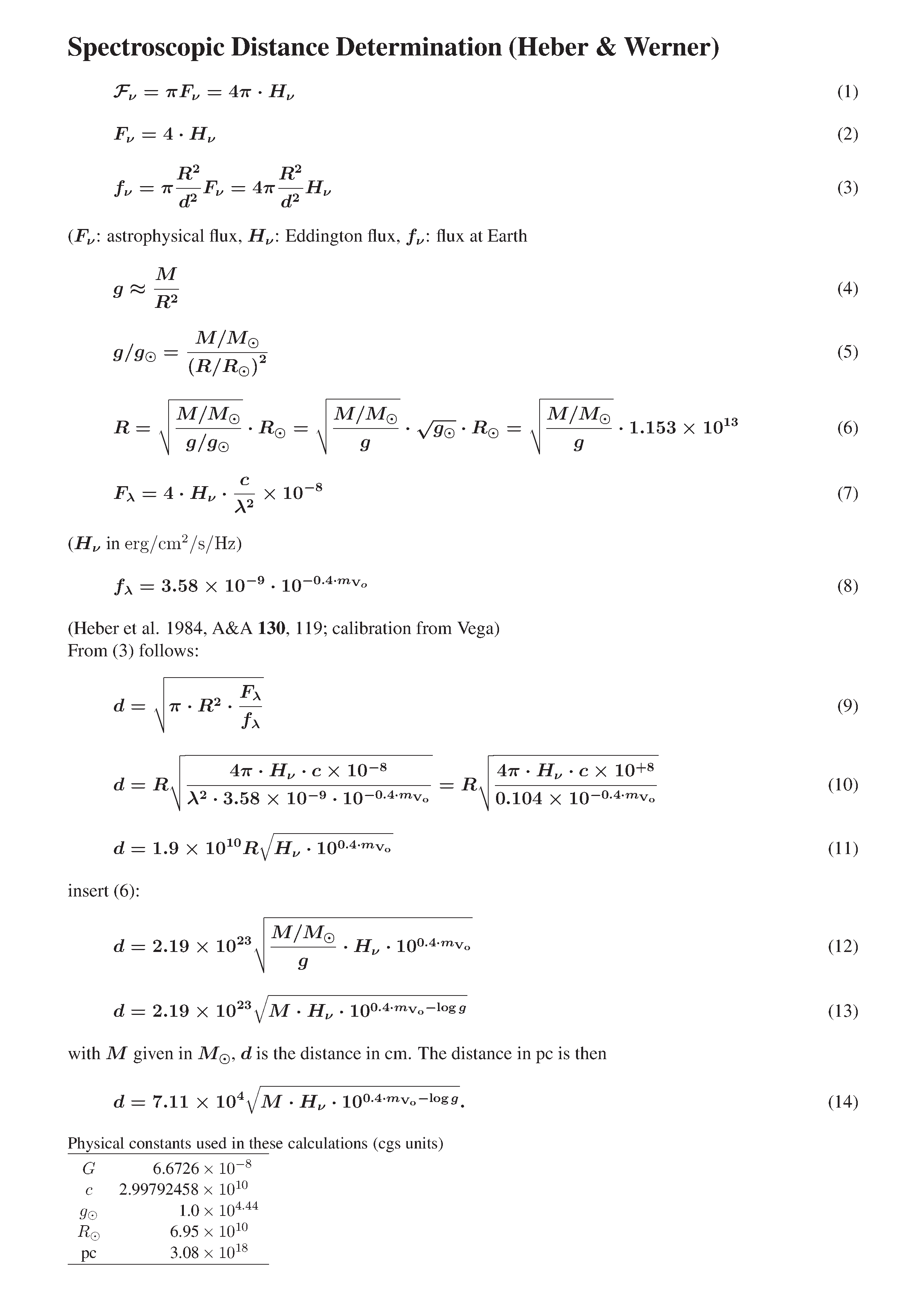
Figure 8 shows that the CS of the PN PRTM 1 is located very close to the Eddington limit. Thus, its cyclic variability may be explained by stellar wind variations (Peña & Ruiz 1998, suggested by) or sudden episodic mass-loss events on a slower timescale (Feibelman 1998) compared to those discovered in case of the CSPN Lo 4 (Werner et al. 1992; Bond 2014, PN G274.3+09.1,). These may also be the reason why Feibelman (1998) identified O vi emission lines in the ultraviolet (UV) spectra obtained with the International Ultraviolet Explorer (IUE) and concluded that the star likely belongs to the so-called O vi sequence. Peña & Ruiz (1998) did not find O vi emission lines in the optical spectra while Boffin et al. (2012) clearly found O vi $\lambda\,5290$ Å (Figs. 5, 7).

For the state-of-the-art spectral analysis of hot stars (Rauch et al. 2013; Rauch et al. 2014, cf., e.g.,), high-resolution spectroscopy in the UV wavelength range is necessary, because most of the stellar metal lines of highly ionized atoms are located there. These allow to measure ionization equilibria of many species. Accurate $T_{\mathrm{eff}}$ and $\log g$ values are a prerequisite for reliable abundance determinations within narrow error limits. In case of the CS of PN PRTM 1, we neglected its variability and exploited a time-averaged optical spectrum. We determined important photospheric parameters that allow to investigate on the nature of the star. However, time-dependent high-resolution UV spectroscopy would significantly improve the spectral analysis and is, thus, highly desirable.

To determine the stellar mass, we compared $T_{\mathrm{eff}}$ and $\log g$ to stellar evolutionary calculations for H-rich post-AGB stars that have recently been presented by Miller Bertolami (2016) (Fig. 8). Two grids with initial metallicities of $Z=0.020$ (about solar) and $Z=0.001$ (halo) yield the same mass of $M=0.73^{+0.16}_{-0.15}\,M_{\odot}$. Thus, it is the one of the heavy-weight H-rich post-AGB stars, located close to the Eddington limit with a high luminosity of $\log(L\,/\,L_{\odot})=4.2\pm 0.4$. The core abundances of the $Z=0.001$ model agree within error limits with the results of this spectral analysis (Table 1). Other models for stellar post-AGB evolution from Vassiliadis & Wood (1994) and Blöcker (1995) give similar values for the stellar mass and luminosity like those of Miller Bertolami (2016).

We calculated the spectroscopic distance following Heber et al. (1984) using $d/\mathrm{pc}=7.11\times 10^{4}\sqrt{H_{\nu}\cdot M\times 10^{0.4\,m_{\mathrm{v}_{0}}-\log g}}$ with $m_{\mathrm{V_{o}}}=m_{\mathrm{V}}-2.175c$, (Peña et al. 1990, $m_{\mathrm{V}}=15.6$, $c(\mathrm{H\beta})=0.06$,) and the Eddington flux $H_{\nu}=1.5\times 10^{-3}\,\mathrm{erg\,cm^{-2}\,s^{-1}\,Hz^{-1}}$ at $\lambda_{\mathrm{eff}}=5454\,\mathrm{\AA}$ of our best model atmosphere. We derived a distance of $d=9.3^{+3.0}_{-2.8}$ kpc and a height below the Galactic plane of $z=5.6^{+1.8}_{-1.7}$ kpc. This agrees within error limits with the previously determined values of Peña et al. (1990, = d ± 5 ⁢ 2 kpc , = | z | ± 3 ⁢ 1.2 kpc ) and verifies that PN PRTM 1 is a halo object.

From the apparent PN diameter of $60″$ (Boffin et al. 2012), we derive its linear radius of $R=1.35^{+0.44}_{-0.40}\,\mathrm{pc}$. Boffin et al. (2012) measured an expansion velocity of $v_{\mathrm{exp}}=30\pm 5\,\mathrm{km/s}$, that yields an expansion time of $44\,000^{+25\,000}_{-17\,500}\,\mathrm{a}$. This is much longer than the post-AGB time of about $120^{+3000}_{\,\,-100}\,\mathrm{a}$, interpolated from evolutionary calculations of Miller Bertolami (2016, = Z 0.02 and = Z 0.001 ,).

The smaller distance determined by Peña et al. (1990) would slightly reduce the discrepancy by a factor of 0.5, however, following Miller Bertolami (2016), a 0.73 $M_{\odot}$ post-AGB star evolves about two orders of magnitude faster after its descend from the AGB. In addition to the huge discrepancy in the theoretical and observed dynamical time scales, Table 1 shows that the final surface abundances of these models do not agree with the result of our spectral analysis. This and the aged, C-poor PN surrounding its relatively massive CS corroborate a presumption that the evolution of the CS of the PN PRTM 1 cannot be explained with a canonical H-rich single star scenario. A late thermal pulse (LTP) that occurred after the first descent from the AGB at still high luminosity, might be responsible for the about solar C and O abundances (Table 1), i.e., enriched C and O in this Halo star.

However, presently no alternative stellar evolutionary models are available that can consistently explain the star’s location in the $\log$ $T_{\mathrm{eff}}$  – $\log g$ plane, its surface composition, and its post-AGB age. To summarize, the evolution of the CS is not understood and needs further investigation but this is not the focus of this paper.

Based on our higher $T_{\mathrm{eff}}$ and $L$ values, a PN reanalysis with an improved ionizing spectrum appears promising to measure the PN abundances (Table 1) again.

The time to calculate synthetic spectra via TMAW to achieve these results was of the order of three weeks. Therefore, all authors and referees should be aware that nowadays possibilities exist for an at least preliminary spectral analysis by means of NLTE model-atmosphere techniques. Any analysis, especially all subsequent interpretations and conclusions, would strongly benefit if such VO services and tools were used.

We thank Henri Boffin and Brent Miszalski who put the mean FORS2 spectrum of the CSPN PRTM 1 at our disposal. The GAVO project had been supported by the Federal Ministry of Education and Research (BMBF) at Tübingen (05 AC 6 VTB, 05 AC 11 VTB) and at Heidelberg (05 AC 6 VHA, 05 A0 8 VHA, 05 AC 11 VHA, 05 AC 14 VHA). We thank the GAVO and AstroGrid-D (http://www.gac-grid.org) teams for support, especially Ulrike Stampa who created the initial version of TheoSSA. The TheoSSA service (http://dc.g-vo.org/theossa) used to retrieve theoretical spectra and the TMAD service (http://astro-uni-tuebingen.de/~TMAD) used to compile atomic data for this paper were constructed as part of the activities of GAVO. Based on data products from observations made with ESO Telescopes at the La Silla Paranal Observatory under programme IDs 078.D$-$0033(A) and 088.D$-$0750(B). This research has made use of NASA’s Astrophysics Data System and of the SIMBAD database and the VizieR catalogue access tool (Ochsenbein et al. 2000, the original description of the VizieR service was published in), operated at CDS, Strasbourg, France.

References

- Asplund et al. (2009) Asplund M., Grevesse N., Sauval A. J., Scott P., 2009, ARA&A, 47, 481
- Auer & Mihalas (1972) Auer L. H., Mihalas D., 1972, ApJS, 24, 193
- Baron et al. (2010) Baron E., Chen B., Hauschildt P. H., 2010, PHOENIX: A General-purpose State-of-the-art Stellar and Planetary Atmosphere Code, Astrophysics Source Code Library (ascl:1010.056)
- Blöcker (1995) Blöcker T., 1995, A&A, 299, 755
- Boffin et al. (2012) Boffin H. M. J., Miszalski B., Jones D., 2012, A&A, 545, A146
- Bond (2014) Bond H. E., 2014, AJ, 148, 44
- Castro-Neves & Draper (2014) Castro-Neves M., Draper P. W., 2014, SPLAT-VO: Spectral Analysis Tool for the Virtual Observatory, Astrophysics Source Code Library (ascl:1402.008)
- Clegg & Middlemass (1987) Clegg R. E. S., Middlemass D., 1987, MNRAS, 228, 759
- Demleitner et al. (2014) Demleitner M., Neves M. C., Rothmaier F., Wambsganss J., 2014, Astronomy and Computing, 7, 27
- Demleitner et al. (2015) Demleitner M., Harrison P., Taylor M., Normand J., 2015, Astronomy and Computing, 10, 88
- Dowler et al. (2015) Dowler P., Bonnarel F., Michel L., Demleitner M., 2015, IVOA DataLink Version 1.0, IVOA Recommendation 17 June 2015 (arXiv:1509.06152)
- Ercolano et al. (2003) Ercolano B., Barlow M. J., Storey P. J., Liu X.-W., Rauch T., Werner K., 2003, MNRAS, 344, 1145
- Feibelman (1998) Feibelman W. A., 1998, PASP, 110, 923
- Hauschildt & Baron (1999) Hauschildt P. H., Baron E., 1999, Journal of Computational and Applied Mathematics, 109, 41
- Hauschildt & Baron (2010) Hauschildt P. H., Baron E., 2010, A&A, 509, A36
- Heber et al. (1984) Heber U., Hunger K., Jonas G., Kudritzki R. P., 1984, A&A, 130, 119
- Hoyer et al. (2017) Hoyer D., Rauch T., Werner K., Kruk J. W., Quinet P., 2017, A&A, 598, A135
- Hubeny (1988) Hubeny I., 1988, Computer Physics Communications, 52, 103
- Hubeny & Lanz (1992) Hubeny I., Lanz T., 1992, A&A, 262, 501
- Hubeny & Lanz (1995) Hubeny I., Lanz T., 1995, ApJ, 439, 875
- Hubeny & Lanz (2011) Hubeny I., Lanz T., 2011, TLUSTY: Stellar Atmospheres, Accretion Disks, and Spectroscopic Diagnostics, Astrophysics Source Code Library (ascl:1109.021)
- Hubeny & Mihalas (2014) Hubeny I., Mihalas D., 2014, Theory of Stellar Atmospheres
- Hubeny et al. (1994) Hubeny I., Hummer D. G., Lanz T., 1994, A&A, 282, 151
- Jahn et al. (2007) Jahn D., Rauch T., Reiff E., Werner K., Kruk J. W., Herwig F., 2007, A&A, 462, 281
- Klepp & Rauch (2011) Klepp S., Rauch T., 2011, A&A, 531, L7
- McDowell et al. (2011) McDowell J., et al., 2011, IVOA Spectrum Data Model Version 1.1, IVOA Recommendation 20 November 2011 (arXiv:1204.3055)
- Méndez (1991) Méndez R. H., 1991, in Michaud G., Tutukov A. V., eds, IAU Symposium Vol. 145, Evolution of Stars: the Photospheric Abundance Connection. p. 375
- Miller Bertolami (2016) Miller Bertolami M. M., 2016, A&A, 588, A25
- Müller-Ringat (2013) Müller-Ringat E., 2013, Dissertation, University of Tübingen, Germany, http://nbn-resolving.de/urn:nbn:de:bsz:21-opus-67747
- Ochsenbein et al. (2000) Ochsenbein F., Bauer P., Marcout J., 2000, A&AS, 143, 23
- Orio et al. (2013) Orio M., et al., 2013, MNRAS, 429, 1342
- Osuna et al. (2005) Osuna P., Barbarisi I., Salgado J., Arviset C., 2005, in Shopbell P., Britton M., Ebert R., eds, Astronomical Society of the Pacific Conference Series Vol. 347, Astronomical Data Analysis Software and Systems XIV. p. 198
- Peña & Ruiz (1998) Peña M., Ruiz M. T., 1998, ApJ, 504, L103
- Peña et al. (1990) Peña M., Torres-Peimbert S., Ruiz M. T., Maza J., 1990, A&A, 237, 454
- Peretz et al. (2016) Peretz U., Orio M., Behar E., Bianchini A., Gallagher J., Rauch T., Tofflemire B., Zemko P., 2016, ApJ, 829, 2
- Plante et al. (2007) Plante R., Linde T., Williams R., Noddle K., 2007, IVOA Identifiers, Version 1.03, IVOA Recommendation, http://www.ivoa.net/documents/REC/Identifiers/Identifiers-20070302.html
- Rauch (1993) Rauch T., 1993, A&A, 276, 171
- Rauch (2008) Rauch T., 2008, in Guainazzi M., Osuna P., eds, Astronomical Spectroscopy and Virtual Observatory. European Space Agency, p. 183 (arXiv:0706.2243)
- Rauch & Deetjen (2003) Rauch T., Deetjen J. L., 2003, in Hubeny I., Mihalas D., Werner K., eds, Astronomical Society of the Pacific Conference Series Vol. 288, Stellar Atmosphere Modeling. p. 103
- Rauch & Nickelt (2009) Rauch T., Nickelt I., 2009, in Baines D., Osuna P., eds, Multi-wavelength Astronomy and Virtual Observatory. p. 49 (arXiv:0901.4202)
- Rauch & Ringat (2011) Rauch T., Ringat E., 2011, in Evans I. N., Accomazzi A., Mink D. J., Rots A. H., eds, Astronomical Society of the Pacific Conference Series Vol. 442, Astronomical Data Analysis Software and Systems XX. p. 563
- Rauch & Ringat (2012) Rauch T., Ringat E., 2012, in Ballester P., Egret D., Lorente N. P. F., eds, Astronomical Society of the Pacific Conference Series Vol. 461, Astronomical Data Analysis Software and Systems XXI. p. 427 (arXiv:1111.5527)
- Rauch et al. (1991) Rauch T., Heber U., Hunger K., Werner K., Neckel T., 1991, A&A, 241, 457
- Rauch et al. (2002) Rauch T., Heber U., Werner K., 2002, A&A, 381, 1007
- Rauch et al. (2007) Rauch T., Ziegler M., Werner K., Kruk J. W., Oliveira C. M., Vande Putte D., Mignani R. P., Kerber F., 2007, A&A, 470, 317
- Rauch et al. (2008) Rauch T., Suleimanov V., Werner K., 2008, A&A, 490, 1127
- Rauch et al. (2009) Rauch T., Nickelt I., Stampa U., Demleitner M., Koesterke L., 2009, in Bohlender D. A., Durand D., Dowler P., eds, Astronomical Society of the Pacific Conference Series Vol. 411, Astronomical Data Analysis Software and Systems XVIII. p. 388 (arXiv:0901.4204)
- Rauch et al. (2010a) Rauch T., Ringat E., Werner K., 2010a, ArXiv 1011.3628,
- Rauch et al. (2010b) Rauch T., Orio M., Gonzales-Riestra R., Nelson T., Still M., Werner K., Wilms J., 2010b, ApJ, 717, 363
- Rauch et al. (2013) Rauch T., Werner K., Bohlin R., Kruk J. W., 2013, A&A, 560, A106
- Rauch et al. (2014) Rauch T., Rudkowski A., Kampka D., Werner K., Kruk J. W., Moehler S., 2014, A&A, 566, A3
- Rauch et al. (2017) Rauch T., Quinet P., Knörzer M., Hoyer D., Werner K., Kruk J. W., Demleitner M., 2017, A&A, 606, A105
- Ringat & Rauch (2010) Ringat E., Rauch T., 2010, in Werner K., Rauch T., eds, American Institute of Physics Conference Series Vol. 1273, American Institute of Physics Conference Series. p. 121, doi:10.1063/1.3527786
- Ringat & Reindl (2013) Ringat E., Reindl N., 2013, in 18th European White Dwarf Workshop.. p. 197
- Ringat et al. (2012) Ringat E., Rauch T., Werner K., 2012, Baltic Astronomy, 21, 341
- Savitzky & Golay (1964) Savitzky A., Golay M. J. E., 1964, Analytical Chemistry, 36, 1627
- Schöning & Butler (1989) Schöning T., Butler K., 1989, A&AS, 78, 51
- Taylor (2005) Taylor M. B., 2005, in Shopbell P., Britton M., Ebert R., eds, Astronomical Society of the Pacific Conference Series Vol. 347, Astronomical Data Analysis Software and Systems XIV. p. 29
- Tody et al. (2007) Tody D., et al., 2007, Simple Spectral Access Protocol Version 1.03, IVOA Recommendation 20 December 2007
- Torres-Peimbert et al. (1990) Torres-Peimbert S., Peña M., Ruiz M. T., Maza J., 1990, in Bulletin of the American Astronomical Society. p. 746
- Tremblay & Bergeron (2009) Tremblay P.-E., Bergeron P., 2009, ApJ, 696, 1755
- Vassiliadis & Wood (1994) Vassiliadis E., Wood P. R., 1994, ApJS, 92, 125
- Werner & Rauch (1997) Werner K., Rauch T., 1997, A&A, 324, L25
- Werner et al. (1991) Werner K., Heber U., Hunger K., 1991, A&A, 244, 437
- Werner et al. (1992) Werner K., Hamann W.-R., Heber U., Napiwotzki R., Rauch T., Wessolowski U., 1992, A&A, 259, L69
- Werner et al. (2003) Werner K., Deetjen J. L., Dreizler S., Nagel T., Rauch T., Schuh S. L., 2003, in Hubeny I., Mihalas D., Werner K., eds, Astronomical Society of the Pacific Conference Series Vol. 288, Stellar Atmosphere Modeling. p. 31
- Werner et al. (2012) Werner K., Dreizler S., Rauch T., 2012, TMAP: Tübingen NLTE Model-Atmosphere Package, Astrophysics Source Code Library (ascl:1212.015)
- Werner et al. (2014) Werner K., Rauch T., Kepler S. O., 2014, A&A, 564, A53
- Werner et al. (2015) Werner K., Rauch T., Kruk J. W., 2015, A&A, 582, A94
- Werner et al. (2016) Werner K., Rauch T., Kruk J. W., 2016, A&A, 593, A104
- Ziegler et al. (2012) Ziegler M., Rauch T., Werner K., Köppen J., Kruk J. W., 2012, A&A, 548, A109
- van Teeseling et al. (1999) van Teeseling A., Gänsicke B. T., Beuermann K., Dreizler S., Rauch T., Reinsch K., 1999, A&A, 351, L27
Appendix A TheoSSA TMAP Web Interface and TMAW WWW Request Web Interface
In general, astronomers are busy and do not have time enough to read extensive manuals or to go through tutorials. Figures 9 to 12 demonstrate how the concept of the VO, to be “easy and intuitive”, has consequently been implemented in the cases of TheoSSA and TMAW. All input fields in Figs. 9 and 11 are clearly and unambiguously labeled and, thus, can easily be filled in.