Generalized Similarity U:
A Non-parametric Test of Association Based on Similarity

We start with a formal set-up. Let $(\Omega,\mathcal{A},P)$ and $(\Psi,\mathcal{G},d)$ be a probability space and a metric space respectively. Consider random elements $Y$ and $G$ taking values on metric space $(\Psi_{Y},\mathcal{G}_{Y},d_{Y})$ and $(\Psi_{G},\mathcal{G}_{G},d_{G})$ with distribution $P_{Y}$ and $P_{G}$ respectively. Here, the random elements can be random variables (e.g., $\Psi=\mathbb{R}$), random vectors (e.g., $\Psi=\mathbb{R}^{p}$), random matrix (e.g., $\Psi=\mathbb{R}^{p\times p}$), random graph (e.g., trees), or random objects (e.g., shapes).

Let $y$ and $g$ denote the realization of the random response element $Y$ and random predictor element $G$. Given a sample of data $\{(y_{i},g_{i})\}_{1\leq i\leq n}$, we are interested in testing the association of response $Y$ and predictor $G$. Since $Y$ and $G$ may not live in a natural vector space, it is not straight forward to construct a regression model, such as $E(Y|G)=f(G)$. However, it is easier to construct similarity measurement for pairs $\{(y_{i},y_{j})\}_{i\neq j}$ and $\{(g_{i},g_{j})\}_{i\neq j}$ with the distance metrics $d_{Y}$ and $d_{G}$. Intuitively, if $Y$ and $G$ are associated, then high similarity between $g_{i}$ and $g_{j}$ should lead to high similarity between $y_{i}$ and $y_{j}$.

The similarity measurement can be defined by a real-valued function quantifying the similarity between two elements. For example, we can define the similarity between $y_{i}$ and $y_{j}$ as $h(y_{i},y_{j})=e^{-d_{Y}(y_{i},y_{j})}$, so that the closer $y_{i}$ and $y_{j}$ are in the metric space, the more similar $y_{i}$ and $y_{j}$ are. Other possible transformations from distance to similarity include inverse transformation $h(y_{i},y_{j})=(d_{Y}(y_{i},y_{j})+\varepsilon)^{-1}$ (for some $\varepsilon>0$) and thresholding transformation $h(y_{i},y_{j})=1_{\{d_{Y}(y_{i},y_{j})<\varepsilon\}}$ ( for some $\varepsilon>0$). Loosely speaking, any monotonically non-increasing function can be used to transform distance to similarity.

Here, we list some examples of similarity measurements.

Example 1 (vector similarity): Let $y_{i},y_{j}\in\mathbb{R}^{p}$. We can use Gaussian kernel ($h(y_{i},y_{j})=exp(-||y_{i}-y_{j}||_{2}^{2})$) or cross-product kernel ($h(y_{i},y_{j})=<y_{i},y_{j}>$) to measure similarity. Here, $<y_{i},y_{j}>$ can be considered as a transformation from Euclidean distance $||\cdot||_{2}^{2}$, using the fact that $<y_{i},y_{j}>=-1/2(||y_{i}-y_{j}||_{2}^{2}-||y_{i}||_{2}^{2}-||y_{j}||_{2}^{2})$.

Example 2 (graph similarity): Let $y=(V,E)$ be a graph with adjacency matrix $A$, where $V$ is the set of vertices and $E$ is the set of edges. For any two graphs $y_{i}$ and $y_{j}$, we can construct a product graph $y_{i}\otimes y_{j}$, with adjacency matrix $A_{i}\otimes A_{j}$. The similarity between the two graphs can be calculated using random walk on the product graph, $h(y_{i},y_{j})=\sum_{k}w_{k}q_{\otimes}^{T}W_{\otimes}^{k}p_{\otimes}$ (Vishwanathan et al., 2010), where $k$ is the length of the random walk, $w_{k}$ is the weight for size-$k$ random walk, $p_{\otimes}$ is the initial probability for vertices on $y_{i}\otimes y_{j}$, $W_{\otimes}$ is the transition probability obtained from $A_{i}\otimes A_{j}$, and $q_{\otimes}$ is the stopping probability for vertices on $y_{i}\otimes y_{j}$. Beside random walk, graph similarity can also be calculated using graphlet and subtree pattern.

Example 3 (image similarity): Image similarity can be calculated from local features and global features of the images by using traditional computer vision techniques such as scale invariant feature transformation (SIFT) and histogram of gradients (HOG). Both SIFT and HOG are human designed feature extraction. With large data sets, we can use modern machine learning methods, such as deep neural network (LeCun et al., 2015), to automatize the feature extraction, and construct more meaningful image similarity from high level representation of image.

Given the predictor elements and the response elements for the subjects $i$ and $j$ ,we denote their response similarity $S_{i,j}$ by,

and denote their predictor similarity $K_{i,j}$ by,$K_{i,j}=f(g_{i},g_{j})$. The similarity measurements $h(\cdotp,\cdotp):\Psi_{Y}\times\Psi_{Y}\to\mathbb{R}$ and $f(\cdotp,\cdotp):\Psi_{G}\times\Psi_{G}\to\mathbb{R}$ can be of a general form as long as they satisfy the finite second moment condition, i.e., $E(h^{2}(Y_{1},Y_{2}))<\infty$ and $E(f^{2}(G_{1},G_{2}))<\infty$, where $Y_{1}$ and $Y_{2}$ ($G_{1}$ and $G_{2}$) are independent identical copy of $Y$ ($G$). We center the response similarity $\tilde{S}_{i,j}=\tilde{h}(y_{i},y_{j})$ by,

and center the predictor similarity, $\tilde{K}_{i,j}=\tilde{f}(g_{i},g_{j})$, in the same manner. Based on the definition of the centered similarity, we can show that $E(\tilde{f}(G_{i},G_{j}))=0$ and $E(\tilde{h}(Y_{i},Y_{j}))=0$ (Supplementary Appendix S1).

We can investigate the relationship of the two similarities using a similarity regression model (Elston et al., 2000; Tzeng et al., 2009),

Since the similarities have been centered, the regression has zero intercept. The association can then be evaluated by testing null hypothesis $b=0$, where $b$ can be estimated by, $\hat{b}={\sum_{i<j}\tilde{K}_{i,j}\tilde{S}_{i,j}}/{\sum_{i<j}(\tilde{K}_{i,j})^{2}}.$ By the form of $\hat{b}$, testing $b=0$ is equivalent to testing the numerator $U_{b}=0$, where $U_{b}=\sum_{i<j}\tilde{K}_{i,j}\tilde{S}_{i,j}$. As we shall see soon, $U_{b}$ is in the same form as the generalized similarity U.

The generalized similarity U (GSU) is defined as the summation of the centered response similarities weighted by the centered predictor similarities,

where $\tilde{K}_{i,j}$ is considered as the weight function and $\tilde{S}_{i,j}$ is considered as the U kernel. In our definition of GSU, the role of response similarity and predictor similarity are interchangeable. In other words, we can also treat $\tilde{S}_{i,j}$ as the weight function and $\tilde{K}_{i,j}$ as the U kernel.

Under the null hypothesis, when the predictor element $G$ is independent of response element $Y$ (i.e., $Y\perp\!\!\!\perp G$), we have $E(U)=\frac{1}{n(n-1)}\sum_{i\neq j}E(\tilde{f}(G_{i},G_{j}))E(\tilde{h}(Y_{i},Y_{j}))=0$. Under alternative hypothesis, when $Y$ is associated with $G$, we expect that the response similarity is concordant with the predictor similarity. In other words, the positive response similarities are weighted heavier and the negative response similarities are weighted lighter, leading to a positive value of U statistic. A statistical test can be formed to test the association, and p-value can be calculated by $P(U>U_{obs})$ under null hypothesis, where $U_{obs}$ is the observed value of $U$.

Define a population parameter $\mu_{U}$ as

It is easy to show that GSU is an unbiased estimator of $\mu_{U}$, i.e., $E(U)=\mu_{U}$. In addition, knowing that $\mu_{U}=E(\tilde{f}(G_{1},G_{2})\tilde{h}(Y_{1},Y_{2}))-E(\tilde{f}(G_{1},G_{2}))E(\tilde{h}(Y_{1},Y_{2})),$ we can consider $\mu_{U}$ as a population covariance. In this sense, a scale invariant “correlation”, $U_{\gamma}$, can be calculated, $U_{\gamma}={\sum_{i\neq j}\tilde{K}_{i,j}\tilde{S}_{i,j}}/{({\sum_{i\neq j}(\tilde{K}_{i,j})^{2}\sum_{i\neq j}(\tilde{S}_{i,j})^{2}})^{1/2}},$ as an indicator of strength of association.

We have already shown that $Y\perp\!\!\!\perp G\Rightarrow\mu_{U}=0$, which ensures the correct type I error. It is of interest now whether $\mu_{U}=0\Rightarrow Y\perp\!\!\!\perp G$, so that we can control type II error (i.e., improve power) and reject null hypothesis whenever $Y\not\!\perp\!\!\!\perp G$. The establishment of $\mu_{U}=0\Rightarrow Y\perp\!\!\!\perp G$ needs additional assumptions on the similarity measurements and metric spaces. For the completeness, we first introduce several preliminaries.

Define a “kernel” as a real symmetric function $h:\Psi\times\Psi\to\mathbb{R}$. A kernel is called positive definite if $\sum_{i,j}^{n}c_{i}c_{j}h(y_{i},y_{j})\geq 0$, $\forall$ $c_{i},c_{j}\in\mathbb{R}$ and $\forall$ $y_{i},y_{j}\in\Psi$. A kernel is called negative definite if $\sum_{i,j}^{n}c_{i}c_{j}h(y_{i},y_{j})\leq 0$, $\forall$ $c_{i},c_{j}\in\mathbb{R},y_{i},y_{j}\in\Psi$ and $\sum_{i}c_{i}=0$.

A positive definite kernel is called strictly positive definite when the equality $\sum_{i,j}^{n}c_{i}c_{j}h(y_{i},y_{j})=0$ implies $c_{i}=0$ $\forall i$. The kernel function here can be used to define similarity measurement. To consider $\mu_{U}=0\Rightarrow Y\perp\!\!\!\perp G$, however, we need the kernel function to exhibit a property of “strong” positive definiteness in the integral form. Using similar notions of Rachev et al. (2013), we define a strongly positive definite kernel as follows.

Definition 1: Let Q be a finite positive measure on $(\Psi,\mathcal{G},d)$ and $q$ be a function integrable with respect to Q. We say $h$ is strongly positive definite if it is positive definite and the equality $\int_{\Psi}\int_{\Psi}h(x,y)q(x)q(y)dQ(x)dQ(y)=0$ implies $q=0$ a.e. $\forall$ Q.

Let $\vartheta$ be a finite signed measure dominated by $Q$ s.t. $d\vartheta=qdQ$. For strongly positive definite kernel $h$, the equality $\int_{\Psi}\int_{\Psi}h(x,y)d\vartheta(x)d\vartheta(y)=0$ implies $\vartheta=0$ $\forall$ $\vartheta$. Now let $\vartheta=P_{GY}-P_{G}P_{Y}$ be a measure on $\Psi_{G}\times\Psi_{Y}$, we can show (in Supplementary Appendix S1) that

If the tensor product kernel $(f\otimes h)\big((g_{1},y_{1}),(g_{2},y_{2})\big)=f(g_{1},g_{2})h(y_{1},y_{2})$ is strongly positive definite, then $\mu_{U}=0$ implies $\vartheta=0$ (i.e., $\mu_{U}=0\Rightarrow Y\perp\!\!\!\perp G$). In fact, we can show $\mu_{U}=0\Rightarrow Y\perp\!\!\!\perp G$ as long as $f$ and $g$ are both strongly positive definite.

Theorem 2: Assume both $f(\cdot,\cdot)$ and $h(\cdot,\cdot)$ are strongly positive definite. Let $\tilde{h}(Y_{1},Y_{2})$ and $\tilde{f}(G_{1},G_{2})$ be the centered similarities as defined in (1). Define $\mu_{U}=E(\tilde{f}(G_{i},G_{j})\tilde{h}(Y_{i},Y_{j}))$. Then, $\mu_{U}=0\Leftrightarrow Y\perp\!\!\!\perp G$.

The proof is given in Appendix A by employing measures embedding into the reproducing kernel Hilbert space. Many popular kernels such as radial basis kernel $h(y_{1},y_{2})=exp(-||y_{1}-y_{2}||_{q})$ ($0<q<2$) are strongly positive definite kernel on $\mathbb{R}^{p}$ (Sriperumbudur et al., 2010). However, the cross product kernel $h(y_{1},y_{2})=<y_{i},y_{j}>$ is not strongly positive definite on $\mathbb{R}^{p}$, by observing that $\int\int<y_{1},y_{2}>d\vartheta(y_{1})d\vartheta(y_{2})=0\Leftrightarrow\int yd\vartheta(y)=0\nRightarrow\vartheta=0$.

For high dimensional data, it is computationally expensive to calculate p-values $P(U>U_{obs})$ using permutation. Here, we derive the asymptotic distribution of GSU under null hypothesis.

By considering the predictor similarity as the weight function and the response similarity as the U kernel, GSU is a weighted U statistic (Lindsay et al., 2008; Wei et al., 2016). More specifically, because its kernel satisfied $Var(E(\tilde{h}(Y_{1},Y_{2})|Y_{2}))=0$ (Supplementary Appendix S1), GSU is a degenerated weighted U statistic. To derive the limiting distribution of GSU, we can decompose the centered response similarity by, $\tilde{h}(y_{1},y_{2})=\sum_{s=1}^{\infty}\lambda_{s}\phi_{s}(y_{1})\phi_{s}(y_{2}),$ where $\{\lambda_{s}\}$ and $\{\phi_{s}(\cdotp)\}$ are eigenvalues and eigenfunctions of the U kennel $\tilde{h}(\cdotp,\cdotp)$, and all the eigenfunctions are orthogonal, i.e., $\int\phi_{s}(y_{1})\phi_{s^{\prime}}(y_{1})dF(y_{1})$ equals 0 if $s\neq s^{\prime}$ and equals 1 if $s=s^{\prime}$. Similarly, we can decompose the centered predictor similarity by, $\tilde{f}(G_{i},G_{j})=\sum_{t=1}^{\infty}\eta_{t}\varphi_{t}(g_{1})\varphi_{t}(g_{2})$. We can then rewrite the GSU as,

where $\varphi_{t}^{\star}(G_{i})=\eta_{t}^{0.5}\varphi_{t}(G_{i})$ and $\phi_{s}^{\star}(Y_{i})=\lambda_{s}^{0.5}\phi_{s}(Y_{i})$. Using the form above, we can show that the limiting distribution of GSU is a weighted sum of independent chi-square random variables. This is the result of theorem 3 below, which is proved in Appendix B.

Theorem 3: Assume $E(h(Y,Y))<\infty$, $E(f(G,G))<\infty$, and $Y\perp\!\!\!\perp G$. Let $\tilde{h}(Y_{1},Y_{2})$ and $\tilde{f}(G_{1},G_{2})$ be the centered similarities as defined in (1). Define U as $U=\frac{1}{n(n-1)}\sum_{i\neq j}\tilde{f}(G_{i},G_{j})\tilde{h}(Y_{i},Y_{j})$. Then, $nU\xrightarrow{D}\sum_{t=1}^{\infty}\eta_{t}\sum_{s=1}^{\infty}\lambda_{s}(\chi_{st}^{2}-1)$, where $\{\chi_{st}^{2}\}$ are independent chi-square random variables with 1 degree of freedom.

Using the similar techniques, we can show that a weighted V statistic in the following form, $V=\frac{1}{n^{2}}\sum_{i,j}\tilde{f}(G_{i},G_{j})\tilde{h}(Y_{i},Y_{j}),$ also converges to a weighted sum of chi-squared variables, i.e., $nV\xrightarrow{D}\sum_{t=1}^{\infty}\eta_{t}\sum_{s=1}^{\infty}\lambda_{s}\chi_{st}^{2}.$

In this subsection, we derive the asymptotic distribution of GSU under the alternative hypothesis, and provide asymptotic power and sample size calculations for association analysis.

Denote $\zeta_{1}=Var(\tilde{f}(G_{1},G_{2})\tilde{h}(Y_{1},Y_{2})|(G_{2},Y_{2}))$. Assume under the alternative hypothesis that $\mu_{U}>0$ and $\zeta_{1}>0$. Using the Hoeffding projection, we can show that GSU asymptotically follows a normal distribution, with mean $\mu_{U}$ and variance $4\zeta_{1}/n$. This is the result of Theorem 4, which is proved in Supplementary Appendix S4.

Theorem 4: Let $\tilde{h}(Y_{1},Y_{2})$ and $\tilde{f}(G_{1},G_{2})$ be the centered similarities as defined in (1). Suppose Y is associated with G, and the following conditions are satisfied: $E(\tilde{f}(G_{1},G_{2})\tilde{h}(Y_{1},Y_{2}))=\mu_{U}>0$, $Var(\tilde{f}(G_{1},G_{2})\tilde{h}(Y_{1},Y_{2}))=\zeta_{0}<\infty$, and $Var(\tilde{f}(G_{1},G_{2})\tilde{h}(Y_{1},Y_{2})|(G_{2},Y_{2}))=\zeta_{1}>0$. Define $U$ as $U=\frac{1}{n(n-1)}\sum_{i\neq j}\tilde{f}(G_{i},G_{j})\tilde{h}(Y_{i},Y_{j})$. Then, $\sqrt{n}(U-\mu_{U})\xrightarrow{D}N(0,4\zeta_{1})$.

The power of GSU at the significance level $\alpha$ can be calculated by, $P\{nU>q_{1-\alpha}\}=\Phi(\frac{n\mu_{U}-q_{1-\alpha}}{2\sqrt{n\zeta_{1}}}),$ where $q_{1-\alpha}$ is the $1-\alpha$ quantile for $\sum_{t=1}^{\infty}\eta_{t}\sum_{s=1}^{\infty}\lambda_{s}(\chi_{st}^{2}-1)$ and $\Phi(\cdotp)$ is the CDF of a standard normal distribution. The sample size required to achieve power $\beta$ can be calculated by solving $\Phi(\frac{n\mu_{U}-q_{1-\alpha}}{2\sqrt{n\zeta_{1}}})\geq\beta$. By denoting $Z_{\beta}$ as the $\beta$ quantile for a standard normal distribution, the required sample size is given by, $n=\min_{n\in N}\left\{n:\>n\geq{(Z_{\beta}\sqrt{\zeta_{1}}+({Z_{\beta}^{2}\zeta_{1}+\mu_{U}q_{1-\alpha}})^{1/2})^{2}}/{\mu_{U}^{2}}\right\}.$

In a sequencing association study, the response element is called phenotype and the predictor element is called genotype. Common forms of phenotype and genotype are scalars or vectors. Suppose that $n$ subjects are sequenced in a study, where we are interested in testing the association of L phenotypic variables ($y_{i,l}$, $1\leq i\leq n$, $1\leq l\leq L$) with M genetic variants ($g_{i,m}$, $1\leq i\leq n$, $1\leq m\leq M$). For each subject $i$, we observe a phenotype vector $y_{i}$ ( $y_{i}=(y_{i,1},y_{i,2},\cdots,y_{i,L})$ ) and a genotype vector $g_{i}$ ( $g_{i}=(g_{i,1},g_{i,2},\cdots,g_{i,M})$). In the special case when $L=1$ (or $M=1$), it is simplified to a univariate analysis (or a single-locus analysis). When $L>1$ (or $M>1$), it extends to a multivariate analysis (or a multi-locus analysis). Here, we allow multiple phenotypes to be of different types (e.g., continuous or categorical), and do not assume any distribution of phenotypes. The number of genetic variants $M$ and the number of phenotypes $L$ can be larger than the sample size. For example, the genetic data can be sequencing data (high dimensional genotype) and the phenotype data can be imaging data (high dimensional phenotype).

The choices for the phenotype similarity $h(\cdotp,\cdotp)$ and the genetic similarity $f(\cdotp,\cdotp)$ are flexible. According to different types of genetic variants and the purpose of the analysis, we can choose different types of phenotype similarities and genetic similarities.

For phenotype similarity, one popular approach is to use a cross product kernel, i.e., $h(y_{i},y_{j})=<y_{i},y_{j}>$ (Tzeng et al., 2009). Yet, as discussed in previous theoretical analysis, cross product kernel may not fit for robust association analysis. Here, we propose a similarity measurement for both categorical and continuous phenotype using radial basis kernel with L1 norm (Laplacian Kernel),

where $\omega_{l}$ represents the weight for the $l$-th phenotypes given based on prior knowledge. If there is no prior knowledge, we can use an equal weight, $\omega_{l}=1/L$. The Laplacian Kernel (LK) based phenotype similarity can be modified to take the correlation among the phenotypes into account, $S_{i,j}^{LK}=exp\left(-\frac{1}{L}d_{ij}^{T}\Gamma d_{ij}\right),$ where $d_{ij}=(|y_{i1}-y_{j1}|^{0.5},\cdots,|y_{iL}-y_{jL}|^{0.5})^{T}$. $\Gamma$ can be chosen to reflect the correlations among the phenotypes. For example, we can define $\Gamma$ as, $\Gamma=(\frac{1}{n}\sum_{i=1}^{n}y_{i}y_{i}^{T})^{-0.5}.$

For the categorical SNVs data, the popular way of measuring genetic similarity is to use IBS function or the weighted IBS function(Lynch and Ritland, 1999). Assuming the genetic variants ($g_{i,m}$, $1\leq i\leq n$, $1\leq m\leq M$) are coded as 0, 1 and 2 for AA, Aa and aa respectively, the IBS-based genetic similarity is defined as, $K_{i,j}^{IBS}=\frac{1}{2M}\sum_{m=1}^{M}2-|g_{i,m}-g_{j,m}|.$ Alternatively, the weighted-IBS (wIBS) genetic similarity can be defined to emphasize the effects of rare variants, $K_{i,j}^{wIBS}=\sum_{m=1}^{M}{w_{m}(2-|g_{i,m}-g_{j,m}|)}/({2\Upsilon}),$ where $w_{m}$ represents the weight for the $m$-th SNV in the SNV-set, and $\Upsilon$ is a scaling constant, defined as $\Upsilon=\sum_{m=1}^{M}w_{m}$. $w_{m}$ is usually defined as a function of minor allele frequency (MAF, denoted as $\gamma_{m}$). For example, the weight $w_{m}$ can be calculated using inverse variance, i.e., $w_{m}=1/\sqrt{\gamma_{m}(1-\gamma_{m})}$. However, IBS-based similarity can not be used for other genetic data, such as copy number variation (count) or expression data (continuous). Here, we propose a unified LK-based genetic similarity by generalizing wIBS,

where $g_{i,m}$ can be categorical, count or continuous variables, and $w_{m}$ can be calculated as function of variance $\sigma_{m}^{2}$ of $g_{m}$, i.e., $w_{m}=1/\sigma_{m}$.

Thus, we defined a unified measurement for genetic similarity and phenotype similarity with Laplacian kernel $exp(-|\cdot-\cdot|)$. Since laplacian kernel is strongly positive definite, we know that (from Theorem 2) the corresponding GSU has the property $\mu_{U}=0\Leftrightarrow G\perp\!\!\!\perp Y$, so that it can control type II error for detection of any types of association. Since Laplacian kernel is bounded similarity measurement, i.e., $0\leq h(\cdot,\cdot)\leq 1$ and $0\leq f(\cdot,\cdot)\leq 1$, we know the regularity conditions in Theorem 3 is satisfied and the asymptotic test for corresponding GSU is robust against distribution assumptions (for large sample size).

Let $S=\{S_{i,j}\}_{n\times n}$ and $K=\{K_{i,j}\}_{n\times n}$ be the matrix form of the phenotype similarity and genetic similarity, the centered similarity matrices $\tilde{S}$ and $\tilde{K}$ can be obtained by, $\tilde{S}=(I-J)S(I-J),$ and $\tilde{K}=(I-J)K(I-J),$ where $I$ is an n-by-n identity matrix, and $J$ is an n-by-n matrix where all elements are $1/n$ (Supplementary Appendix S5). Then GSU can be expressed as, $U=\frac{1}{n(n-1)}\sum_{i\neq j}\tilde{K}_{i,j}\tilde{S}_{i,j}.$ In this form, $U$ can be viewed as a sum of the element-wise product of the two matrices, $\tilde{K}_{0}$ and $\tilde{S}_{0}$, which are obtained by assigning 0 to the diagonal elements of matrices $\tilde{K}$ and $\tilde{S}$.

To allow for covariates adjustment, we can perform two sided projection on the zero-diagonal centered similarity matrices, $\tilde{K}_{0}$ and $\tilde{S}_{0}$. Suppose that there are $P$ covariates that need to be adjusted. Let $X=\{x_{i,p}\}_{n\times P}$ represents the covariate matrix, we can calculate the covariate centered similarity matrices by (Supplementary Appendix S6), $\hat{S}=(I-X(X^{T}X)^{-1}X^{T})\tilde{S}_{0}(I-X(X^{T}X)^{-1}X^{T}),$ and $\hat{K}=(I-X(X^{T}X)^{-1}X^{T})\tilde{K}_{0}(I-X(X^{T}X)^{-1}X^{T}).$ The covariate adjusted GSU can be expressed as,

We include the diagonal terms in the covariate-adjusted similarities because they also contain the similarity information after the adjustment. In fact, the covariate-adjusted GSU is a weighted V statistic, and its asymptotic distribution can be attained similarly as weighted U statistic. We use matrix eigen-decomposition to approximate the eigen-values in function decomposition. Let $\{\hat{\lambda}_{s}\}$ and $\{\hat{\eta}_{t}\}$ be the eigen-values for matrices $\hat{K}$ and $\hat{S}$ respectively, the limiting distribution of $U$ is given by (Supplementary Appendix S7),

where $\{\chi_{st}^{2}\}$ are independent chi-square random variables with 1 degree of freedom. The p-value can be calculated by using the Davies’ method (Davies, 1980), the Liu’s method(Liu et al., 2009) or the Kuonen’s method(Kuonen, 1999). To facilitate the high dimensional data analysis, we developed a C++ package based on GSU (https://github.com/changshuaiwei/gsu).

To mimic real genetic structure, we used genetic data from the 1000 Genome Project(Abecasis et al., 2010). Based on the genetic data, we then simulated phenotype values. In particular, we used a 1Mb region of the genome (Chromosome 17: 7344328-8344327) from the 1000 Genome Project. For each simulation replicate, we randomly chose a 30kb segment from the 1Mb region and formed a SNV-set for the analysis, in which only rare variants (i.e., $MAF<0.05$) are used except otherwise specified. From the SNV-set, we set a proportion of the SNVs as causal. A number of individuals were randomly chosen from the total 1092 individuals as the simulation sample to study the performance of the methods. We set sample size $n=50$ by default.

To investigate the robustness against different phenotype distributions, we simulated four types of phenotypes:

1. 1.

   A binary-distributed phenotype (denoted as B), by $logit(P(Y_{i}=1))=\mu_{i}+G_{i}^{T}\beta$,

2. 2.

   A Poisson-distributed phenotype (denoted as P), by $Y_{i}\sim Pois(a_{i}),log(a_{i})=\mu_{i}+G_{i}^{T}\beta$,

3. 3.

   A Gaussian-distributed phenotype (denoted as G), by $Y_{i}=\mu_{i}+G_{i}^{T}\beta+\varepsilon_{i},\>\varepsilon_{i}\sim N(0,\sigma^{2})$,

4. 4.

   And a Cauchy-distributed phenotype (denoted as C), by $Y_{i}\sim cauchy(a_{i},b),\>a_{i}=\mu_{i}+G_{i}^{T}\beta$,

Here, $Y_{i}$ and $G_{i}$ were the phenotype value and the genotype vector (coded as 0, 1, and 2) for the $i$-th individual, respectively. We set $\mu_{i}=0$ except otherwise specified. $\beta$ were the effects of the SNVs, which were sampled from a uniform distribution with a mean of $\mu_{\beta}$ and a variance of $\sigma_{\beta}^{2}$.

Three sets of simulations were performed. In simulation I, we considered a single phenotype; in simulation II, we considered multivariate phenotype; in simulation III, we considered multivariate phenotype under the influence of confounding effects. Details of simulation settings are in Supplementary Appendix S8.

We evaluated the performance of GSU by comparing it with variance component score (VCscore) test under univariate or multivariate linear mixed model (Wu et al., 2011; Maity et al., 2012). For each simulation, we created 1000 simulation replicates to evaluate type I error and power. Type I error rates and powers are calculated using percentage of p-values smaller than a given threshold (e.g., 0.05) under null models and alternative models respectively.

The type I error rates and powers are summarized in Table 1. GSU had a well-controlled type I error (around 0.05) for all 4 phenotypes, while VCscore had an inflated type I error rates (0.113) for Cauchy-distributed phenotype and over-conservative type I error rates (0.005) for Binary-distributed phenotype.

For the disease model where half of the causal SNVs were deleterious (Table 1), GSU had slightly lower power than VCscore for Gaussian-distributed (0.258 v.s. 0.345) and Poisson-distributed phenotype (0.506 v.s. 0.651), but had significantly higher power than VCscore for Cauchy-distributed (0.503 v.s. 0.21) and Binary-distributed phenotype(0.402 v.s. 0.083). The same comparison was observed for the second disease model in which a majority of the SNVs were deleterious.

We performed additional simulations by including both common and rare variants (Supplementary Table S4). Under this setting, the power of VCscore increased significantly for Binary phenotype (0.764), though still lower than that of GSU (0.807). GSU attained higher power than VCscore for Poisson (0.813 v.s. 0.795) and Cauchy (0.885 v.s. 0.573) phenotype. Nevertheless, GSU was still less powerful than VCscore for Gaussian phenotype (0.853 v.s. 0.878).

The type I error rates and powers for the multivariate analysis are summarized in Table 2. Similar to the results of the univariate analysis, GSU can correctly control type I error at the level of 0.05 (Table 2), while VCscore had inflated type I error when the phenotype contained variables with heavy tailed distribution (e.g., CGG and BCG). GSU attained higher power than VCscore for BBG, CGG and BCG phenotypes, and similar power as VCscore for BPP phenotype.

We examined the type I error rates at more stringent significance levels (Table 3) by simulating 1 million replicates. In general, GSU can control the type I error better than VCscore. For example, at $5\times 10^{-3}$ and for BPP phenotype, GSU had type I error near $5\times 10^{-3}$ (i.e., $7.4\times 10^{-3}$), while, VCscore had type I error much higher than $5\times 10^{-3}$ (i.e., $1.1\times 10^{-2}$). While simulation demonstrated robustness of GSU over VCscore on controlling type I error, we observe GSU has slightly inflated type I errors at $5\times 10^{-3}$ level. We suspect this is because of the small sample size. We therefore conducted another set of simulation with sample size of 200, and the results showed type I errors of GSU are better controlled for stringent significant levels under larger sample size (Supplementary Table S5).

To separate influences of different distributions, we also compared GSU and VCscore when phenotype have the same distributions (i.e., BBB, CCC, GGG, PPP). The results (Supplementary Table S6) are similar to those for univariate phenotype. In general, GSU can control type I errors better than VCscore. GSU had slightly lower power than VCscore for GGG phenotype (0.882 v.s. 0.958) and PPP phenotype (0.862 v.s. 0.966), but attained significantly higher power for BBB phenotype (0.862 v.s. 0.26) and CCC phenotype (0.724 v.s. 0.284). We further increased the dimension of phenotype to 10 for each type, and the comparisons showed that GSU have better control of type I error and attain higher power for most cases (Supplementary Figure S1).

We summarized the type I errors in Table 4. Without covariates adjustment, both methods had inflated type I errors. With covariates adjustment, GSU showed robustness against confounding effects for all 4 multivariate phenotypes, with type I errors ranging from 0.056 to 0.061. VCscore can control type I error for BBG phenotype (0.054), but had inflated type I errors, ranging from 0.174 to 0.322, for the other 3 multivariate phenotypes.

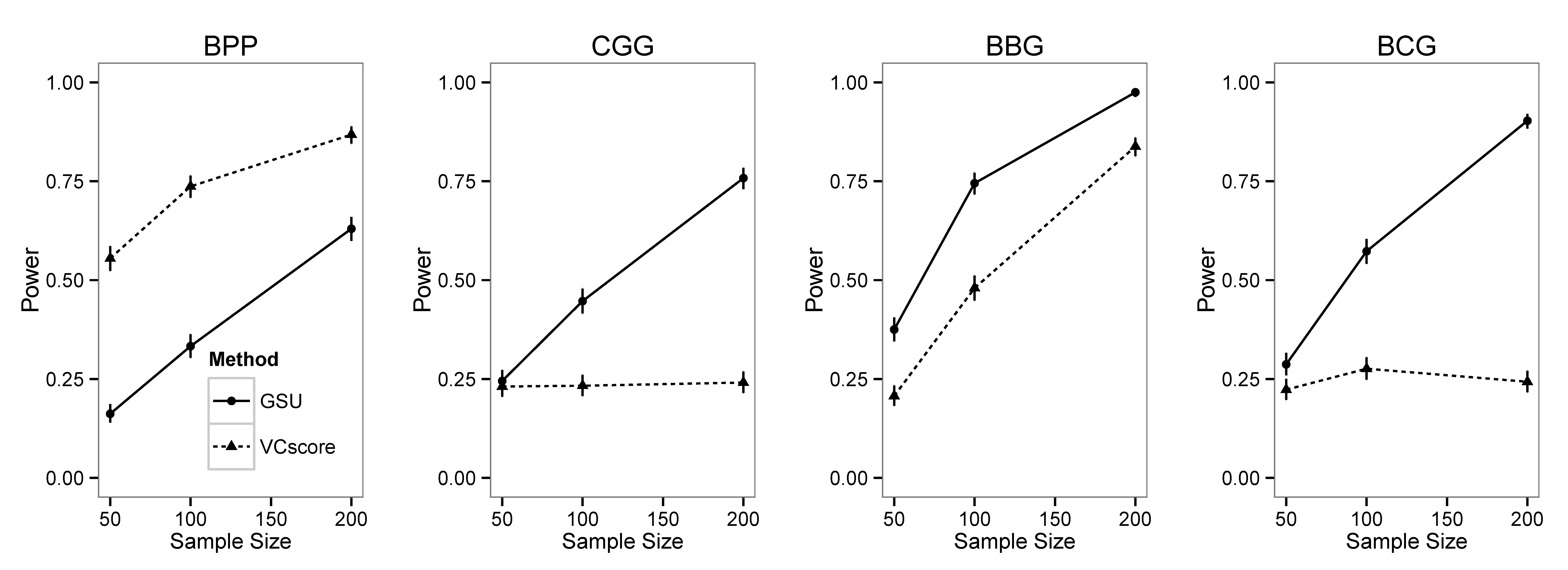
In Figure 1, we generated the power curves by plotting the powers of the two methods against different sample sizes (50 to 200). GSU has higher power than VCscore for different sample sizes and multivariate phenotypes, except for BPP phenotype. The “higher power” of VCscore for BPP phenotype is due to the fact that VCscore has inflated type I error (i.e., 0.322, as shown in Table 4).

References

- Abecasis et al. (2010) Abecasis, G. R., Altshuler, D., Auton, A., Brooks, L. D., Durbin, R. M., Gibbs, R. A., Hurles, M. E., and McVean, G. A. (2010). A map of human genome variation from population-scale sequencing. Nature 467, 1061–73.
- Berlinet and Thomas-Agnan (2011) Berlinet, A. and Thomas-Agnan, C. (2011). Reproducing kernel Hilbert spaces in probability and statistics. Springer Science & Business Media.
- Cirulli and Goldstein (2010) Cirulli, E. T. and Goldstein, D. B. (2010). Uncovering the roles of rare variants in common disease through whole-genome sequencing. Nature Reviews Genetics 11, 415–425.
- Davies (1980) Davies, R. B. (1980). Algorithm as 155: The distribution of a linear combination of x2 random variables. Journal of the Royal Statistical Society. Series C (Applied Statistics) 29, 323–333.
- Dick and Agrawal (2008) Dick, D. M. and Agrawal, A. (2008). The genetics of alcohol and other drug dependence. Alcohol Research & Health 31, 111.
- Elston et al. (2000) Elston, R. C., Buxbaum, S., Jacobs, K. B., and Olson, J. M. (2000). Haseman and elston revisited. Genetic epidemiology 19, 1–17.
- Kuonen (1999) Kuonen, D. (1999). Saddlepoint approximations for distributions of quadratic forms in normal variables. Biometrika 86, 929–935.
- LeCun et al. (2015) LeCun, Y., Bengio, Y., and Hinton, G. (2015). Deep learning. Nature 521, 436–444.
- Li et al. (2011) Li, M., Ye, C., Fu, W., Elston, R. C., and Lu, Q. (2011). Detecting genetic interactions for quantitative traits with u-statistics. Genetic epidemiology 35, 457–468.
- Lin (1997) Lin, X. (1997). Variance component testing in generalised linear models with random effects. Biometrika 84, 309–326.
- Lindsay et al. (2008) Lindsay, B. G., Markatou, M., Ray, S., Yang, K., and Chen, S. C. (2008). Quadratic distances on probabilities: A unified foundation. Annals of Statistics 36, 983–1006.
- Liu et al. (2009) Liu, H., Tang, Y. Q., and Zhang, H. H. (2009). A new chi-square approximation to the distribution of non-negative definite quadratic forms in non-central normal variables. Computational Statistics & Data Analysis 53, 853–856.
- Lynch and Ritland (1999) Lynch, M. and Ritland, K. (1999). Estimation of pairwise relatedness with molecular markers. Genetics 152, 1753–1766.
- Lyons (2013) Lyons, R. (2013). Distance covariance in metric spaces. The Annals of Probability 41, 3284–3305.
- Maity et al. (2012) Maity, A., Sullivan, P. E., and Tzeng, J. Y. (2012). Multivariate phenotype association analysis by marker-set kernel machine regression. Genetic Epidemiology 36, 686–695.
- Rachev et al. (2013) Rachev, S. T., Klebanov, L., Stoyanov, S. V., and Fabozzi, F. (2013). The methods of distances in the theory of probability and statistics. Springer Science & Business Media.
- Schaid et al. (2005) Schaid, D. J., McDonnell, S. K., Hebbring, S. J., Cunningham, J. M., and Thibodeau, S. N. (2005). Nonparametric tests of association of multiple genes with human disease. American Journal of Human Genetics 76, 780–793.
- Sriperumbudur et al. (2010) Sriperumbudur, B. K., Gretton, A., Fukumizu, K., Schölkopf, B., and Lanckriet, G. R. (2010). Hilbert space embeddings and metrics on probability measures. The Journal of Machine Learning Research 11, 1517–1561.
- Tao et al. (2015) Tao, R., Zeng, D., Franceschini, N., North, K. E., Boerwinkle, E., and Lin, D.-Y. (2015). Analysis of sequence data under multivariate trait-dependent sampling. Journal of the American Statistical Association 110, 560–572.
- Tong et al. (2016) Tong, X., Wei, C., and Lu, Q. (2016). Genome-wide joint analysis of single-nucleotide variant sets and gene expression for hypertension and related phenotypes. BMC proceedings 10, 125.
- Tzeng et al. (2009) Tzeng, J.-Y., Zhang, D., Chang, S.-M., Thomas, D. C., and Davidian, M. (2009). Gene-trait similarity regression for multimarker-based association analysis. Biometrics 65, 822–832.
- van der Vaart and Wellner (2000) van der Vaart, A. and Wellner, J. A. (2000). weak convergence and empirical processes. Springer, 2 edition.
- Vishwanathan et al. (2010) Vishwanathan, S. V. N., Schraudolph, N. N., Kondor, R., and Borgwardt, K. M. (2010). Graph kernels. The Journal of Machine Learning Research 11, 1201–1242.
- Wang et al. (2015) Wang, Y., Liu, A., Mills, J. L., Boehnke, M., Wilson, A. F., Bailey-Wilson, J. E., Xiong, M., Wu, C. O., and Fan, R. (2015). Pleiotropy analysis of quantitative traits at gene level by multivariate functional linear models. Genetic epidemiology 39, 259–275.
- Wei et al. (2016) Wei, C., Elston, R. C., and Lu, Q. (2016). A weighted u statistic for association analyses considering genetic heterogeneity. Statistics in Medicine .
- Wei and Lu (2015) Wei, C. and Lu, Q. (2015). A generalized similarity u test for multivariate analysis of sequencing data. arXiv preprint arXiv:1505.01179 .
- Wu et al. (2011) Wu, M. C., Lee, S., Cai, T. X., Li, Y., Boehnke, M., and Lin, X. H. (2011). Rare-variant association testing for sequencing data with the sequence kernel association test. American Journal of Human Genetics 89, 82–93.
- Wu et al. (2013) Wu, M. C., Maity, A., Lee, S., Simmons, E. M., Harmon, Q. E., Lin, X., Engel, S. M., Molldrem, J. J., and Armistead, P. M. (2013). Kernel machine snp-set testing under multiple candidate kernels. Genetic epidemiology 37, 267–275.
- Zhang et al. (2010) Zhang, H. P., Liu, C. T., and Wang, X. Q. (2010). An association test for multiple traits based on the generalized kendall’s tau. Journal of the American Statistical Association 105, 473–481.
Appendix 1
Due to space limit, we here only sketch the proofs. Detailed proofs can be found at Supplementary Appendix S2 and S3.
Appendix A: embedding into Hilbert Space
For each positive definite kernel , we can construct a unique reproducing kernel Hilbert space (RKHS) with reproducing kernel (Berlinet and Thomas-Agnan, 2011), such that, 1) , , 2) , , . We can write , and then represent a measure as an element in RKHS (Lyons, 2013) using an embedding map : , s.t.,. Further, if is strongly positive definite, we can show the mapping is one-to-one, i.e., .
Let and . We can then write as, , where, . If , then we know , i.e.,
We then can show, by repeatedly using measure embedding, that , i.e., .
Appendix B: Proof of Theorem 3
Because of the orthogonality of and the fact that , we can show . Similarly, . Under the null hypothesis, predictor element () is independent of response element (). Therefore, for and ,
and
Therefore, for any finite subset of , the multivariate random variable converges to a multivariate normal distribution.
Then, we need to show the convergence is uniform. Notice that, . Under the condition , the infinite countable sequence of function is a Donsker class (Theorem 2.13.1 in van der Vaart and Wellner (2000)). Therefore, the empirical process, , converges weakly to the Gaussian process with mean zero and covariance function, . With this uniform convergence (for all and ), we can show that,
where are i.i.d chi-squared random variables with a d.f. of 1.