Radial basis function collocation method for decoupled fractional Laplacian wave equations

For homogeneous acoustic media, the nearly constant-$Q$ decoupled fractional Laplacian equation describing the stress field $\sigma(x,t)$ ($x\in\mathbb{R}^{d}$) is written by [7]

where $\eta=-c_{0}^{2\gamma}\omega_{0}^{-2\gamma}\cos(\pi\gamma)$, $\tau=-c_{0}^{2\gamma-1}\omega_{0}^{-2\gamma}\sin(\pi\gamma)$, and $c=c_{0}\cos({\pi\gamma}/{2})$ is the phase velocity depending on the velocity $c_{0}$ at the reference angular frequency $\omega_{0}$. The quality factor $Q$, which is related to $\gamma$ by $\gamma=\arctan(1/Q)/\pi$, is used to describe how fast the attenuation will be. The smaller the $Q$ is, the faster the wave attenuates. As $Q$ goes to the infinity, $\gamma$ will be zero, which indicates that Eq.(1) will reduce to a standard wave equation (with no attenuation) due to $\tau=0$ for $\gamma=0$. Oppositely, for $Q=0$, namely $\gamma=0.5$, the equation will be a diffusion equation, because $\eta$ is zero now. Note that for homogeneous media, $c_{0}$ and $Q$ are both independent of spatial variable and thus constants.

Under the condition $|\gamma\ln(\omega/\omega_{0})|\ll 1$, the dispersive phase velocity $c$ and attenuation coefficient $\alpha$ arising from Eq.(1) are given by

It is seen that the velocity and the attenuation are both frequency dependent for non-zero fractional order $\gamma$.

The reason why it is called the decoupled equation is that the equation can be decoupled into the attenuation-dominated equation

and the dispersion-dominated equation

The decoupling effects are helpful for developing stable $Q$-compensated reverse time migration [16].

There have been three typical definitions of the fractional Laplacian: integral or Riesz definition (see Eq.(25.56) of [17]), directional definition (see [18, 13] and Eq.(26.24) of [17]), and spectral definition ([19, 20]). Other definitions can be found in [21]. Ref.[15] compares the aforementioned three typical definitions defined on bounded domains and concludes that the first two are equivalent but differ from the third one.

In the paper we restrict to the directional definition, given by [13]

where the scaling constant before the integral is [22]

and the fractional directional derivative is given by

where $\nabla$ is the gradient operator, and the fractional directional integral $I_{\boldsymbol{\theta}}^{\beta}(\cdot)$ is defined by (for $\beta\in(0,1)$)

where $\Gamma(\cdot)$ is the Euler Gamma function. The directional definition is equivalent to the Riesz one and it is easy to be approximated by using RBF collocation method.

Great care should be taken for setup of boundary conditions for the governing equation (1). For pure Dirichlet problem, to guarantee uniqueness and existence of the solution, a nonlocal boundary condition should be given with the exterior condition and terminal observation time $T$ [23]:

For simplicity, we here assume that the stress vanishes in the exterior. It should be noted that the above boundary condition could still be insufficient to ensure the well-posedness of the mathematical problem, since the highest order of the space derivative in our wave equation exceeds two because of the presence of the dispersion term $(-\nabla^{2})^{\gamma+1}(\cdot)$ for $\gamma\in(0,0.5)$. An additional boundary condition could be needed. For example, the local-form normal condition

where $n$ is the outward unit normal, can be added. Other boundary conditions, say, the prescribed fractional normal derivative [24], is also possible. It should be noted that how to prove the well-posedness of the present wave equation given boundary conditions is still an open problem. Nevertheless, from the numerical experiments, we see that for zero boundary conditions, the normal boundary condition (10) can be discarded. Therefore, in the rest of the paper, we will only adopt the zero boundary condition (9).

The initial conditions are given by

The stress field to be solved $\sigma(x,y,t)$ is approximated by the weighted sum of the RBFs $\phi(r)$:

where $\{(x_{j},y_{j})\}$ are a group of source points located in the computational domain, and $M$ and $N$ are the numbers of points on the domain and boundary, respectively. The point set $\{(x_{i},y_{i})\}$ include collocation points, which coincide with the source points. The RBF $\phi(\cdot)$ only depends on the distance (or the relative location) between the collocation point $(x_{i},y_{i})$ and the source point $(x_{j},y_{j})$, namely $r_{ij}$, and therefore the collocation or source points are not constrained by any mesh or element. Additionally, $\lambda_{j}(t)$ is the time-dependent expansion coefficients to be evaluated.

Substituting RBF approximation (12) in our wave equation (1) and in the boundary condition (9) and using the finite difference scheme for the temporal discretization, we lead to the following approximating scheme

The RBF expansion coefficient $\lambda_{j}^{n}$ means $\lambda_{j}((n-1)\Delta t)$ and the quantity $\phi_{ij}$ is defined by $\phi(r_{ij})$. $(-\nabla^{2})^{\beta}\phi_{ij}$ represents $[(-\nabla^{2})^{\beta}\phi](x_{i},y_{i})$ where $\beta$ can be $\gamma+1$ or $\gamma+1/2$. The first $M$ equations correspond to the approximation of the governing equation (1) and the last $N$ equations approximate the zero-valued boundary condition (9). $\Delta t$ is the time step of the finite difference scheme. We here assume the velocity is spatially variable, i.e. $c_{i}=c(x_{i},y_{i})$, in order to use the model to simulate the layered media. An external force term $f_{i}^{n}=f(x_{i},y_{i},(n-1)\Delta t)$ is also considered. We have a trick here. The collocation (or source) points are placed simply on the boundary $\partial\Omega$ rather than the whole exterior $\mathbb{R}^{d}\setminus\Omega$. This trick avoids the choice of points outside $\Omega$. Without the trick, we need to place some points in the outward neighbourhood of boundary. To reduce the number of points, we remove the neighbourhood and find that the removing has little effect on the numerical results when zero-valued boundary condition is considered.

Rearranging the above approximating scheme, we have the matrix form ($n=2,3,...,L$ where $T=L\Delta t$)

$\boldsymbol{\Phi}_{d}$ is a matrix formed by the RBFs with domain-type collocation points and all the source points, i.e. $[\phi_{ij}]$ with $i=1,2,\cdots,M;j=1,2,\cdots,M+N$. Similarly, $\boldsymbol{\Phi}_{b}$ is given by $[\phi_{ij}]$ with $i=M+1,M+2,\cdots,M+N;j=1,2,\cdots,M+N$. The $M\times M$ diagonal matrix $\mathbf{C}$ has the velocities evaluated at domain-type collocation points to be its diagonals, namely $[c_{i}]$ with $i=1,2,\cdots,M$. Corresponding to the $n$- th time layer, $\boldsymbol{\lambda}^{n}=[\lambda_{j}^{n}]$ and $\mathbf{f}^{n}=[f_{i}^{n}]$ are $(M+N)$- and $M$- dimensional column vectors, respectively. $\boldsymbol{\Phi}_{\gamma+1}$ and $\boldsymbol{\Phi}_{\gamma+1/2}$ are the $M\times(M+N)$ matrices formed by the fractional derivatives of the RBFs, and the next subsection will show how to compute these matrices.

The first expansion coefficient vector $\boldsymbol{\lambda}^{1}$ is obtained by solving the RBF interpolation problem

where the vector formed by the initial values is denoted by $\boldsymbol{\sigma}_{0}=\sigma_{0}(x_{i},y_{i})$ for $i=1,2,\cdots,M+N$. The second expansion coefficient vector $\boldsymbol{\lambda}^{2}$ coincides with the first one due to the initial condition $\frac{\partial\sigma(x,y,0)}{\partial t}=0$, i.e.

Through the iterations of the RBF expansion coefficients $\boldsymbol{\lambda}^{n}$ in (14) starting from $\boldsymbol{\lambda}^{1},\boldsymbol{\lambda}^{2}$, we can derive the coefficients for any given time $t_{n}=(n-1)\Delta t$. Finally, the use of RBF expansion formula (12) leads us to the approximate stress at any time-space coordinates.

The computation of fractional Laplacian of RBFs is not usually an easy task, particularly when an unsuitable definition of fractional Laplacian is considered. For instance, if one considers the Riesz definition, which is a hyper-singular integral, even though the integrand is completely known, the hypersingularity prevents further approximation. Fortunately, the directional definition (5) enables a straightforward approximation of fractional Laplacian. The definition indicates that one can approximate the fractional Laplacian within two steps: Get the fractional directional derivative of the RBFs and then evaluate the integral with respect to differential direction $\boldsymbol{\theta}$.

Ref.[13] approximates the fractional directional derivative of RBFs using Gauss-Jacobi quadrature under the assumption that the fractional directional derivative is defined in Caputo sense. Note that the Caputo fractional derivative is a regularized version of the Riemann-Liouville (RL) fractional derivative and does not completely preserve the nonlocality or the memory effect of the fractional derivative. For example, a RL fractional derivative of a constant is a power function, whereas a Caputo fractional derivative of a constant is zero, which is the same case as the integer-order derivative. Consideration of the RL fractional derivative could be preferable in mathematical modeling. To compute the RL derivative of RBFs, we adopt the vector Grünwald scheme proposed in [25].

In two dimensional case, the scheme is written by

The above scheme has the first order accuracy, i.e., $O(h)$ truncation error. The symbol $[a]$ gets the closest integer to the fraction $a$. $d(x_{i},y_{i},\theta,\Omega)$ is the distance from the collocation point $(x_{i},y_{i})$ to the boundary of the computing domain along the direction $(\cos\theta,\sin\theta)$. The second step is to evaluate the integration of the above directional derivative with respect to $\theta$. The integral can be accurately approximated by using trapezoidal rule since $D_{\theta}^{\beta}(\cdot)$ is periodic for $\theta$. We thus have the quadrature formula ($\theta_{l}=2\pi l/N_{t}$)

where $N_{t}+1$ compound trapezoidal quadrature points are used. Letting the fractional order $\beta$ be $\gamma+1$ and $\gamma+1/2$, the index $i$ go from $1$ to $M$, and the index $j$ go from $1$ to $M+N$, we can compute all the elements of the matrices $\boldsymbol{\Phi}_{\gamma+1}$ and $\boldsymbol{\Phi}_{\gamma+1/2}$ aforementioned.

Consider the synthetic solution $\sigma_{e}=\exp(-t)x^{3}(1000-x)^{3}y^{3.6}(1000-y)^{3.6}$ on a square domain $\Omega=(0,1000)^{2}$. The external force term $f(x,y,t)$ can be directly computed by

with the velocity $c=3000m/s$, the quality factor $Q=10$, the acoustic density $\rho_{0}=1g/cm^{3}$, and the reference frequency $\omega_{0}=60rad/s$. The computation of fractional Laplacian of a known function has been detailed in subsection 3.2. The step size $h$ in the vector Grünwald scheme (17) is set to be $10^{-3}$ when computing the fractional Laplacian of RBFs. For computing the fractional Laplacian of $\sigma_{e}$, we halve the step size in order to make the external force $f$ as accurate as possible. Similarly, for computing the fractional Laplacian of RBFs, we use 21 trapezoidal quadrature points ($N_{t}=20$) while for the fractional Laplacian of $\sigma_{e}$, we use 41 quadrature points. Previous numerical experiments show that $h=1m$ and $N_{t}=20$ can produce acceptable approximation accuracy. In the following examples, we keep these two parameters unchanged.

We test the RBF solution accuracy on the grid points of a $10\times 10$ regular grid on $\Omega$. The maximum absolute error and the average relative error are defined by $||\boldsymbol{\sigma}-\boldsymbol{\sigma}_{e}||_{\infty}$ and $||\boldsymbol{\sigma}-\boldsymbol{\sigma}_{e}||_{2}/||\boldsymbol{\sigma}_{e}||_{2}$, respectively. $\boldsymbol{\sigma}$ and $\boldsymbol{\sigma}_{e}$ are the vectors formed by the approximate solutions and the synthetic solutions evaluated at the test points.

Fig.1(left) shows the variation of error against the number of collocation (or source) points, namely $M+N$. Fig.1(right) shows the total CPU time for computing the fractional Laplacian of RBFs, say,$\boldsymbol{\Phi}_{\gamma+1}$ and for directly solving the linear system (14) once. We see that the RBF collocation method achieves acceptable accuracy for a small number of collocation points. But, the time complexity for generating the matrices whose entries are fractional Laplacian of RBFs is $O(N_{t}M(M+N))$ and the complexity for directly solving the linear system is $O((M+N)^{3})$.

Consider a homogeneous medium of size $1000m\times 1000m$ with acoustic velocity $c_{0}=2000m/s$ and quality factor $Q=100$. Let the initial wavefield be

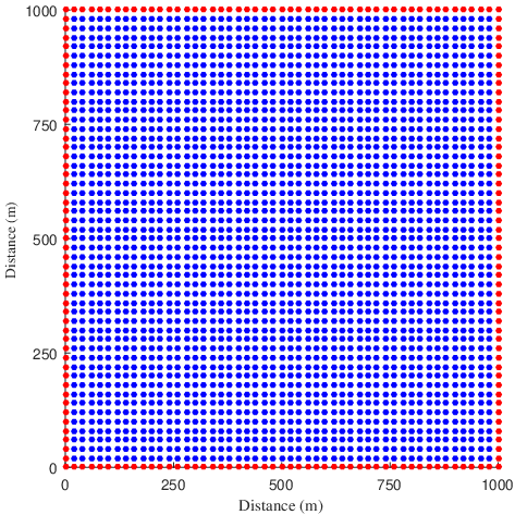
with $r^{2}=(x-x_{s})^{2}+(y,y_{s})^{2}$. The source location of the seismic wave is $(x_{s},y_{s})$. The parameter $f_{0}$ is set to be $f_{0}=5$. The plot of the initial wavefield is shown in Fig.2(a). In the rest of the paper, all the simulations use this initial wavefield, and $f_{0}=5$ and $f_{0}=12$ are used for homogeneous and multi-layer media, respectively. The external force is ignored, i.e. $f(x,y,t)\equiv 0$. The locations of collocation points are given in Fig.2(b).

Fig.3 compares the wavefields computed by RBF collocation and Fourier pseudospectral method. We see that the two methods produce the waves that have same phase but different amplitudes. The difference probably arises from the different boundary conditions considered in these two methods. The RBF collocation method considers the nonlocal zero-valued boundary condition, and the solutions on the exterior are zero; in contrast, the pseudospectral method assumes periodic boundary condition and the solutions on the exterior are simply the copies of the solution on the internal domain.

The numerical stability of the RBF collocation method for long-time simulations is studied and illustrated in Fig.4(a,b). Additionally, the influence of the quality factor on the solutions is also considered, which can be observed from Fig.4(c).

Fig. 5 shows the wavefields simulated by using RBF method for two different irregular domains. These results are only used to illustrate the utility of the RBF collocation method for solving irregular domain problem. It should be noted that we make the first attempt to solve the decoupled fractional Laplacian equation on irregular domains.

We consider the media with acoustic velocity varying layer by layer. The synthetic velocity data are extracted from the synthetic dataset of the HESS VTI model [26]. The geometric size of the medium in the original HESS model is quite large, and to reduce the computational cost of solving the fractional Laplacian wave equation, we select a small part of medium. Fig.6 (top) shows a $36000m\times 15000m$ medium considered in HESS model and what we consider are two subregions: Region A with regular boundary and Region B with irregular boundary.

The second row of the subfigures in Fig.6 displays, respectively, the synthetic velocity field of Region A, and the simulated wavefields at $t=400,500,600ms$. The initial wave source is located at the center of right side. The reflection and refraction of the wave on the interfaces of different layers can be clearly seen.

Fig.7 shows the simulations on Region B. The source is located on the curved boundary. The left top subfigure shows the synthetic velocity distribution, and the rest of the subfigures give the simulated wavefields at $t=400,600,800ms$.

It can be seen that the RBF collocation method can be employed to simulate the wave in the media with spatially dependent velocity.

References

- [1] T. L. Szabo, Time domain wave equations for lossy media obeying a frequency power law, Journal of the Acoustical Society of America 96 (1) (1994) 491–500.
- [2] W. Chen, S. Holm, Modified szabo¡¯s wave equation models for lossy media obeying frequency power law, The Journal of the Acoustical Society of America 114 (5) (2003) 2570–2574.
- [3] W. Chen, S. Holm, Fractional laplacian time-space models for linear and nonlinear lossy media exhibiting arbitrary frequency power-law dependency, The Journal of the Acoustical Society of America 115 (4) (2004) 1424–1430.
- [4] S. Holm, S. P. Näsholm, A causal and fractional all-frequency wave equation for lossy media, The Journal of the Acoustical Society of America 130 (4) (2011) 2195–2202.
- [5] S. Holm, S. P. Nasholm, Comparison of fractional wave equations for power law attenuation in ultrasound and elastography, Ultrasound in Medicine and Biology 40 (4) (2014) 695–703.
- [6] B. E. Treeby, B. T. Cox, Modeling power law absorption and dispersion for acoustic propagation using the fractional laplacian, Journal of the Acoustical Society of America 127 (5) (2010) 2741–2748.
- [7] T. Zhu, J. M. Harris, Modeling acoustic wave propagation in heterogeneous attenuating media using decoupled fractional laplacians, Geophysics 79 (3) (2014) T105–T116.
- [8] W. Chen, J. Fang, G. Pang, S. Holm, Fractional biharmonic operator equation model for arbitrary frequency-dependent scattering attenuation in acoustic wave propagation., Journal of the Acoustical Society of America 141 (1) (2017) 244.
- [9] J. M. Carcione, A generalization of the fourier pseudospectral method, Geophysics 75 (6) (2010) A53–A56.
- [10] H. Chen, H. Zhou, Q. Li, Y. Wang, Two efficient modeling schemes for fractional laplacian viscoacoustic wave equation, Geophysics 81 (5) (2016) T233–T249.
- [11] E. J. Kansa, Multiquadrics¡ªa scattered data approximation scheme with applications to computational fluid-dynamics¡ªii solutions to parabolic, hyperbolic and elliptic partial differential equations, Computers & Mathematics with Applications 19 (8) (1990) 147–161.
- [12] W. Chen, Z. J. Fu, C. S. Chen, Recent advances on radial basis function collocation methods, Springer Berlin Heidelberg, 2014.
- [13] G. Pang, W. Chen, Z. Fu, Space-fractional advection-dispersion equations by the kansa method, Journal of Computational Physics 293 (2015) 280–296.
- [14] B. Fornberg, N. Flyer, Solving pdes with radial basis functions, Acta Numerica 24 (2015) 215–258.
- [15] A. Lischke, G. Pang, F. Song, C. Glusa, M. Gulian, X. Zheng, Z. Mao, W. Cai, M. M. Meerschaert, M. Ainsworth, G. E. Karniadakis, What is the fractional laplacian?, submitted.
- [16] T. Zhu, J. M. Harris, B. Biondi, Q-compensated reverse-time migration, Geophysics 79 (3) (2014) S77–S87.
- [17] A. Kilbas, O. Marichev, S. Samko, Fractional integral and derivatives (theory and applications), Gordon and Breach, Switzerland 1 (993) (1993) 1.
- [18] M. M. Meerschaert, D. A. Benson, B. Bäumer, Multidimensional advection and fractional dispersion, Physical Review E 59 (5) (1999) 5026.
- [19] M. Ilic, F. Liu, I. Turner, V. Anh, Numerical approximation of a fractional-in-space diffusion equation, i, Fractional Calculus and Applied Analysis 8 (3) (2005) 323–341.
- [20] F. Song, C. Xu, G. E. Karniadakis, Computing fractional laplacians on complex-geometry domains: Algorithms and simulations, SIAM Journal on Scientific Computing 39 (4) (2017) A1320–A1344.
- [21] M. Kwaśnicki, Ten equivalent definitions of the fractional laplace operator, Fractional Calculus and Applied Analysis 20 (1) (2017) 7–51.
- [22] G. Pang, W. Chen, K. Sze, Gauss–jacobi-type quadrature rules for fractional directional integrals, Computers & Mathematics with Applications 66 (5) (2013) 597–607.
- [23] C. Bucur, Some observations on the green function for the ball in the fractional laplace framework, arXiv preprint arXiv:1502.06468.
- [24] S. Dipierro, X. Ros-Oton, E. Valdinoci, Nonlocal problems with neumann boundary conditions, arXiv preprint arXiv:1407.3313.
- [25] M. M. Meerschaert, J. Mortensen, H.-P. Scheffler, Vector grünwald formula for fractional derivatives, Fractional Calculus and Applied Analysis 7 (1) (2004) 61–82.
- [26] F. Liu, S. A. Morton, S. Jiang, L. Ni, J. P. Leveille, Decoupled wave equations for p and sv waves in an acoustic vti media, Seg Technical Program Expanded Abstracts (2009) 2844–2848.
- [27] J. Berenger, Perfectly matched layer for the fdtd solution of wave-structure interaction problems, IEEE Transactions on Antennas and Propagation 44 (1) (1996) 110–117.