跳到论文正文
W Papers独立论文阅读器 arXiv:1801.00843 论文正文 计算阅读时间 · 0%
引用这篇论文根据当前论文元数据生成,正式投稿前建议核对。


License: arXiv.org perpetual non-exclusive license
arXiv:1801.00843v1 [cs.CC] 02 Jan 2018

The geometry of rank decompositions of matrix multiplication II: 3×33\times 3 matricesThanks: Landsberg supported by NSF grant DMS-1405348. Ballard supported in part by an appointment to the Sandia National Laboratories Truman Fellowship in National Security Science and Engineering, sponsored by Sandia Corporation (a wholly owned subsidiary of Lockheed Martin Corporation) as Operator of Sandia National Laboratories under its U.S. Department of Energy Contract No. DE-AC04-94AL85000.

Grey Ballard Address: PO Box 7311, Department of Computer Science, Wake Forest University, Winston-Salem, NC 27109 Email address: ballard@wfu.edu , Christian Ikenmeyer Address: Max Planck Institute for Informatics, Saarland Informatics Campus, Building E1.4, D-66123 Saarbrücken, Germany Email address: cikenmey@mpi-inf.mpg.de , J.M. Landsberg Address:  Department of Mathematics
Texas A&M University
Mailstop 3368
College Station, TX 77843-3368, USA
Email address: jml@math.tamu.edu
and Nick Ryder Address: Department of Mathematics
UC Berkeley
Email address: nick.ryder@berkeley.edu
Abstract.

This is the second in a series of papers on rank decompositions of the matrix multiplication tensor. We present new rank 2323 decompositions for the 3×33\times 3 matrix multiplication tensor M⟨3⟩M_{\langle 3\rangle}. All our decompositions have symmetry groups that include the standard cyclic permutation of factors but otherwise exhibit a range of behavior. One of them has 11 cubes as summands and admits an unexpected symmetry group of order 12.

We establish basic information regarding symmetry groups of decompositions and outline two approaches for finding new rank decompositions of M⟨𝐧⟩M_{\langle\mathbf{n}\rangle} for larger 𝐧\mathbf{n}.

Key words and phrases: 
matrix multiplication complexity, alternating least squares, MSC 68Q17, 14L30, 15A69

1. Introduction

This is the second in a planned series of papers on the geometry of rank decompositions of the matrix multiplication tensor M⟨𝐧⟩∈ℂ𝐧2​⊗​ℂ𝐧2​⊗​ℂ𝐧2M_{\langle\mathbf{n}\rangle}\in\mathbb{C}^{\mathbf{n}^{2}}{\mathord{\otimes}}\mathbb{C}^{\mathbf{n}^{2}}{\mathord{\otimes}}\mathbb{C}^{\mathbf{n}^{2}}. Our goal is to obtain new rank decompositions of M⟨𝐧⟩M_{\langle\mathbf{n}\rangle} by exploiting symmetry. For a tensor T∈ℂm​⊗​ℂm​⊗​ℂmT\in\mathbb{C}^{m}{\mathord{\otimes}}\mathbb{C}^{m}{\mathord{\otimes}}\mathbb{C}^{m}, the rank of TT is the smallest rr such that T=∑j=1raj​⊗​bj​⊗​cjT=\sum_{j=1}^{r}a_{j}{\mathord{\otimes}}b_{j}{\mathord{\otimes}}c_{j}, with aj,bj,cj∈ℂma_{j},b_{j},c_{j}\in\mathbb{C}^{m}. The rank of M⟨𝐧⟩M_{\langle\mathbf{n}\rangle} is a standard complexity measure of matrix multiplication, in particular, it governs the total number of arithmetic operations needed to multiply two matrices.

In this paper we present rank 23 decompositions of M⟨3⟩M_{\langle 3\rangle} that have large symmetry groups, in particular all admit the standard cyclic ℤ3\mathbb{Z}_{3}-symmetry of permuting the three tensor factors. Although many rank 23 decompositions of M⟨3⟩M_{\langle 3\rangle} are known [15, 13], none of them was known to admit the standard cyclic ℤ3\mathbb{Z}_{3}-symmetry.

We describe techniques to determine symmetry groups of decompositions and to determine if two decompositions are in the same family, as defined in §4. We also develop a framework for using representation theory to write down new rank decompositions for M⟨𝐧⟩M_{\langle\mathbf{n}\rangle} for all 𝐧\mathbf{n}. Similar frameworks are also being developed implicitly and explicitly in [5] and [12].

As discussed below, decompositions come in families. DeGroote [8] has shown, in contrast to M⟨3⟩M_{\langle 3\rangle}, the family generated by Strassen’s decomposition is the unique family of rank seven decompositions of M⟨2⟩M_{\langle 2\rangle}. Unlike M⟨2⟩M_{\langle 2\rangle}, it is still not known if the tensor rank of M⟨3⟩M_{\langle 3\rangle} is indeed 2323. The best lower bound on the rank is 1616 [17]. There have been substantial unsuccessful efforts to find smaller decompositions by numerical methods. While some researchers have taken this as evidence that 2323 might be optimal, it just might be the case that rank 2222 (or smaller) decompositions might be much rarer than border rank 2222 decompositions, and so using numerical search methods, and given initial search points, when they converge, with probability nearly one would converge to border rank decompositions.

In this paper we focus on decompositions with standard cyclic symmetry: viewed as a trilinear map, matrix multiplication is (X,Y,Z)↦trace⁡(X​Y​Z)(X,Y,Z)\mapsto\operatorname{trace}(XYZ), where X,Y,ZX,Y,Z are 𝐧×𝐧\mathbf{n}\times\mathbf{n} matrices. Since trace⁡(X​Y​Z)=trace⁡(Y​Z​X)\operatorname{trace}(XYZ)=\operatorname{trace}(YZX), the matrix multiplication tensor M⟨𝐧⟩∈ℂ𝐧2​⊗​ℂ𝐧2​⊗​ℂ𝐧2=M​a​tn×n⊗​3M_{\langle\mathbf{n}\rangle}\in\mathbb{C}^{\mathbf{n}^{2}}{\mathord{\otimes}}\mathbb{C}^{\mathbf{n}^{2}}{\mathord{\otimes}}\mathbb{C}^{\mathbf{n}^{2}}=Mat_{n\times n}^{{\mathord{\otimes}}3} has a ℤ3\mathbb{Z}_{3} symmetry by cyclically permuting the three factors. If one applies this cyclic permutation to a tensor decomposition of M⟨𝐧⟩M_{\langle\mathbf{n}\rangle}, it is transformed to another decomposition of M⟨𝐧⟩M_{\langle\mathbf{n}\rangle}. When a decomposition is transformed to itself, we say the decomposition has cyclic symmetry or ℤ3s​t​d\mathbb{Z}_{3}^{std}-invariance.

In §2 we present three of our examples. We explain the search methods used in §3. We then discuss techniques for determining symmetry groups in §4 and determine the symmetry groups of our decompositions in §5. Our searches sometimes found equivalent decompositions but in different coordinates, and the same techniques enabled us to identify when two decompositions are equivalent. Further techniques for studying decompositions are presented in §6 and §8, respectively in terms of configurations of points in ℙn−1\mathbb{P}^{n-1} and eigenvalues. In §7, we precisely describe the subspace of ℤ3\mathbb{Z}_{3}-invariant tensors in M​a​tn×n⊗​3Mat_{n\times n}^{{\mathord{\otimes}}3}, as well as the subspaces invariant under other finite groups. In an appendix §A, we present additional decompositions that we found.

Why search for decompositions with symmetry?

There are many examples where the optimal decompositions (or expressions) of tensors with symmetry have some symmetry. This is true of M⟨2⟩M_{\langle 2\rangle} [6, 4], the monomial x1⋯xnx_{1}\cdots x_{n} [19], also see [16, §7.1], the optimal determinantal expression of perm3\operatorname{perm}_{3} [18], and other cases. In any case, imposing the symmetry i) reduces the size of the search space, and ii) provides a guide for constructing decompositions through the use of “building blocks”.

Notation and conventions

A,B,C,U,V,WA,B,C,U,V,W are vector spaces, A∗A^{*} is the dual vector space to AA, G​L​(A)GL(A) denotes the group of invertible linear maps A→AA\rightarrow A, S​L​(A)SL(A) the maps with determinant one, and P​G​L​(A)=G​L​(A)/{ℂ​IdA\0}PGL(A)=GL(A)/\{\mathbb{C}\operatorname{Id}_{A}\backslash 0\} the group of projective transformations of projective space ℙ​A\mathbb{P}A. The action of G​L​(A)GL(A) on A​⊗​A∗A{\mathord{\otimes}}A^{*} descends to an action of P​G​L​(A)PGL(A). If a∈Aa\in A, [a][a] denotes the corresponding point in projective space. 𝔖d\mathfrak{S}_{d} denotes the permutation group on dd elements and ℤd\mathbb{Z}_{d} denotes the cyclic group of order dd. For X⊂ℙ​VX\subset\mathbb{P}V, X^⊂V\hat{X}\subset V denotes its pre-image under the projection map union the origin. X(×r)X^{(\times r)} denotes the quotient X×r/𝔖rX^{\times r}/\mathfrak{S}_{r}. We write S​Lm=S​L​(ℂm)SL_{m}=SL(\mathbb{C}^{m}), G​Lm=G​L​(ℂm)GL_{m}=GL(\mathbb{C}^{m}), and HS​Lm⊂S​LmH^{SL_{m}}\subset SL_{m} is the subgroup of diagonal matrices. For a matrix aa, ajia^{i}_{j} denotes the entry in the ii-th row and jj-th column.

Acknowledgements

Work on this paper began during the fall 2014 semester program Algorithms and Complexity in Algebraic Geometry at the Simons Institute for the Theory of Computing. We thank the Institute for bringing us together and making this paper possible.

2. Examples

2.1. A rank 2323 decomposition of M⟨3⟩M_{\langle 3\rangle} with ℤ4×ℤ3\mathbb{Z}_{4}\times\mathbb{Z}_{3} symmetry

Let ℤ4a0⊂G​L3⊂G​L3×3\mathbb{Z}_{4}^{a_{0}}\subset GL_{3}\subset GL_{3}^{\times 3} be generated by

(1) a0=(00−110−101−1),{a_{0}}=\begin{pmatrix}0&0&-1\\ 1&0&-1\\ 0&1&-1\end{pmatrix},

where the action on x​⊗​y​⊗​zx{\mathord{\otimes}}y{\mathord{\otimes}}z where x,y,zx,y,z are 3×33\times 3-matrices is x⊗y⊗z↦a0xa0−1⊗a0ya0−1⊗a0za0−1x{\mathord{\otimes}}y{\mathord{\otimes}}z\mapsto{a_{0}}x{a_{0}}{}^{-1}{\mathord{\otimes}}{a_{0}}y{a_{0}}{}^{-1}{\mathord{\otimes}}{a_{0}}z{a_{0}}{}^{-1} and let ℤ3s​t​d\mathbb{Z}_{3}^{std} denote the standard cyclic symmetry.

Here is the decomposition, we call it 𝒮ℤ4×ℤ3{\mathcal{S}}_{\mathbb{Z}_{4}\times\mathbb{Z}_{3}}:

(2) M⟨3⟩=\displaystyle M_{\langle 3\rangle}= −(00−110−101−1)⊗​3\displaystyle-\begin{pmatrix}0&0&-1\\ 1&0&-1\\ 0&1&-1\end{pmatrix}^{{\mathord{\otimes}}3}
(3) +ℤ4a0/ℤ2a02⋅(010010000)⊗​3\displaystyle+\mathbb{Z}_{4}^{a_{0}}/\mathbb{Z}_{2}^{a_{0}^{2}}\cdot\begin{pmatrix}0&1&0\\ 0&1&0\\ 0&0&0\end{pmatrix}^{{\mathord{\otimes}}3}
(4) +ℤ4a0⋅(100000000)⊗​3\displaystyle+\mathbb{Z}_{4}^{a_{0}}\cdot\begin{pmatrix}1&0&0\\ 0&0&0\\ 0&0&0\end{pmatrix}^{{\mathord{\otimes}}3}
(5) +ℤ4a0⋅(0−101−10000)⊗​3\displaystyle+\mathbb{Z}_{4}^{{a_{0}}}\cdot\begin{pmatrix}0&-1&0\\ 1&-1&0\\ 0&0&0\end{pmatrix}^{{\mathord{\otimes}}3}
(6) +ℤ3s​t​d×ℤ4a0⋅(000001000)⊗(000000−110)⊗(00001−101−1).\displaystyle+\mathbb{Z}_{3}^{std}\times\mathbb{Z}_{4}^{{a_{0}}}\cdot\begin{pmatrix}0&0&0\\ 0&0&1\\ 0&0&0\end{pmatrix}{\mathord{\otimes}}\begin{pmatrix}0&0&0\\ 0&0&0\\ -1&1&0\end{pmatrix}{\mathord{\otimes}}\begin{pmatrix}0&0&0\\ 0&1&-1\\ 0&1&-1\end{pmatrix}.

The decomposition is a sum of 2323 terms, each of which is a trilinear form on matrices. For example, the term (000001000)​⊗​(000000−110)​⊗​(00001−101−1)\begin{pmatrix}0&0&0\\ 0&0&1\\ 0&0&0\end{pmatrix}{\mathord{\otimes}}\begin{pmatrix}0&0&0\\ 0&0&0\\ -1&1&0\end{pmatrix}{\mathord{\otimes}}\begin{pmatrix}0&0&0\\ 0&1&-1\\ 0&1&-1\end{pmatrix} sends a triple of matrices (x,y,z)(x,y,z) to the number x23​(y32−y31)​(z22−z23+z32−z33)x_{23}(y_{32}-y_{31})(z_{22}-z_{23}+z_{32}-z_{33}). This expresses M⟨3⟩M_{\langle 3\rangle} in terms of five ℤ4×ℤ3\mathbb{Z}_{4}\times\mathbb{Z}_{3}-orbits, of sizes 1,2,4,4,121,2,4,4,12.

2.2. An element of the 𝒮ℤ4×ℤ3{\mathcal{S}}_{\mathbb{Z}_{4}\times\mathbb{Z}_{3}} family with a0a_{0} diagonalized

It is also illuminating to diagonalize a0a_{0}, in other words decompose the decomposition with respect to the ℤ4\mathbb{Z}_{4} action: In the following plot each row of 3×33\times 3 matrices forms an orbit under the ℤ4\mathbb{Z}_{4}-action. In the first four rows are the eleven 3×33\times 3 matrices that appear as cubes in the decomposition. In remaining 4 rows each of the four columns forms three rank one tensors by tensoring the three matrices in the column in three different orders: 1-2-3, 2-3-1, and 3-1-2.

Each complex number in each matrix is depicted by plotting its position in the complex plane. To help identify the precise position, a square is drawn with vertices (−12,−12)(-\frac{1}{2},-\frac{1}{2}), (12,−12)(\frac{1}{2},-\frac{1}{2}), (−12,12)(-\frac{1}{2},\frac{1}{2}), (12,12)(\frac{1}{2},\frac{1}{2}). To quickly identify the absolute value of a complex number they are color coded:
Symbol for the complex number absolute value 1 12\frac{1}{\sqrt{2}} 12​2\frac{1}{2{\sqrt{2}}} 12\frac{1}{2} 52​2\frac{\sqrt{5}}{2\sqrt{2}}

Numbers with a blue background are the sum of two numbers with a yellow background. Numbers with a purple background are twice the numbers with a yellow background. Numbers with a red background are twice the numbers with a blue background. Numbers with a green background are the sum of a number with a yellow background and a number with a blue background.

Matrix cells with zeros are left empty.

2.3. A cyclic-invariant decomposition in the Laderman family

Let 𝒮L​a​d​e​r​m​a​n{\mathcal{S}}_{Laderman} denote the rank 2323 Laderman decomposition of M⟨3⟩M_{\langle 3\rangle}. By [4] the symmetry group of this decomposition (see §4) is Γ𝒮L​a​d​e​r​m​a​n=(ℤ2×ℤ2)⋊(ℤ3⋊ℤ2)≃𝔖4\Gamma_{{\mathcal{S}}_{Laderman}}=(\mathbb{Z}_{2}\times\mathbb{Z}_{2})\rtimes(\mathbb{Z}_{3}\rtimes\mathbb{Z}_{2})\simeq\mathfrak{S}_{4}, where ℤ2×ℤ2⊂S​L3×3\mathbb{Z}_{2}\times\mathbb{Z}_{2}\subset SL_{3}^{\times 3}. We found a decomposition, which we call 𝒮L​a​d​e​r−ℤ3s​t​d{\mathcal{S}}_{Lader-\mathbb{Z}_{3}^{std}} that we identified as a ℤ3s​t​d\mathbb{Z}_{3}^{std}-invariant member of the Laderman family in the sense of §4.

Let

τ23=(100001010),ϵ2=(1000−10001),τ13=(001010100),\tau_{23}=\begin{pmatrix}1&0&0\\ 0&0&1\\ 0&1&0\end{pmatrix},\ \epsilon_{2}=\begin{pmatrix}1&0&0\\ 0&-1&0\\ 0&0&1\end{pmatrix},\ \tau_{13}=\begin{pmatrix}0&0&1\\ 0&1&0\\ 1&0&0\end{pmatrix},\

Let ϕ⁡(x​⊗​y​⊗​z)=τ13​x​τ13​⊗​τ13​y​⊗​z​τ13\phi(x{\mathord{\otimes}}y{\mathord{\otimes}}z)=\tau_{13}x\tau_{13}{\mathord{\otimes}}\tau_{13}y{\mathord{\otimes}}z\tau_{13}, and let ζ⁡(x​⊗​y​⊗​z)=ϵ2​yT​ϵ2​⊗​ϵ2​xT​ϵ2​⊗​ϵ2​zT​ϵ2\zeta(x{\mathord{\otimes}}y{\mathord{\otimes}}z)=\epsilon_{2}y^{T}\epsilon_{2}{\mathord{\otimes}}\epsilon_{2}x^{T}\epsilon_{2}{\mathord{\otimes}}\epsilon_{2}z^{T}\epsilon_{2}. Let π\pi be the generator of ℤ3s​t​d\mathbb{Z}_{3}^{std}. Let Γ\Gamma denote the group generated by π,ϕ\pi,\phi, and ζ\zeta.

(7) M⟨3⟩\displaystyle M_{\langle 3\rangle} =(000010000)⊗​3\displaystyle=\begin{pmatrix}0&0&0\\ 0&1&0\\ 0&0&0\end{pmatrix}^{{\mathord{\otimes}}3}
(8) +Γ/(ℤ3π⋊ℤ2ζ)⋅(000000001)⊗​3\displaystyle+\Gamma/(\mathbb{Z}_{3}^{\pi}\rtimes\mathbb{Z}_{2}^{\zeta})\cdot\begin{pmatrix}0&0&0\\ 0&0&0\\ 0&0&1\end{pmatrix}^{{\mathord{\otimes}}3}
(9) +Γ/(ℤ3π⋊ℤ2ζ)⋅(−110−100000)⊗​3\displaystyle+\Gamma/(\mathbb{Z}_{3}^{\pi}\rtimes\mathbb{Z}_{2}^{\zeta})\cdot\begin{pmatrix}-1&1&0\\ -1&0&0\\ 0&0&0\end{pmatrix}^{{\mathord{\otimes}}3}
(10) +Γ/(ℤ2ϕ⋊ℤ2ζ)⋅(0−10000000)⊗(1−101−1−1011)⊗(000100000)\displaystyle+\Gamma/(\mathbb{Z}_{2}^{\phi}\rtimes\mathbb{Z}_{2}^{\zeta})\cdot\begin{pmatrix}0&-1&0\\ 0&0&0\\ 0&0&0\end{pmatrix}{\mathord{\otimes}}\begin{pmatrix}1&-1&0\\ 1&-1&-1\\ 0&1&1\end{pmatrix}{\mathord{\otimes}}\begin{pmatrix}0&0&0\\ 1&0&0\\ 0&0&0\end{pmatrix}
(11) +Γ/ℤ3π⋅(100100000)⊗​3\displaystyle+\Gamma/\mathbb{Z}_{3}^{\pi}\cdot\begin{pmatrix}1&0&0\\ 1&0&0\\ 0&0&0\end{pmatrix}^{{\mathord{\otimes}}3}

These five orbits are respectively of sizes 1,4,4,6,81,4,4,6,8. There are five ℤ3s​t​d\mathbb{Z}_{3}^{std} invariant terms, one from each of (7),(8),(9) and two from (11) because ζ\zeta preserves ℤ3s​t​d\mathbb{Z}_{3}^{std}-invariance.

We originally found this decomposition by numerical methods. The incidence graphs discussed in §4.3 gave us evidence that it should be in the Laderman family, and then it was straightforward to find the transformation that exchanged 𝒮L​a​d​e​r​m​a​n{\mathcal{S}}_{Laderman} and 𝒮L​a​d​e​r−ℤ3s​t​d{\mathcal{S}}_{Lader-\mathbb{Z}_{3}^{std}}, namely x​⊗​y​⊗​z↦τ12​x​⊗​y​ϵ2​τ12​⊗​τ12​ϵ2​z​τ12x{\mathord{\otimes}}y{\mathord{\otimes}}z\mapsto\tau_{12}x{\mathord{\otimes}}y\epsilon_{2}\tau_{12}{\mathord{\otimes}}\tau_{12}\epsilon_{2}z\tau_{12}. See §4.3 for more discussion. As shown in in [4], Γ\Gamma is isomorphic to 𝔖4\mathfrak{S}_{4} and these are all the symmetries of the Laderman family. Translated to 𝒮L​a​d​e​r​m​a​n{\mathcal{S}}_{Laderman} as presented in [4], these five orbits are respectively {19}\{19\}, {20,21,22,23}\{20,21,22,23\}, {4,7,12,16}\{4,7,12,16\}, {1,3,6,10,11,14}\{1,3,6,10,11,14\} and {2,5,8,9,13,15,17,18}\{2,5,8,9,13,15,17,18\}.

Remark 2.1.

As pointed out in [20], there are similarities between this decomposition and Strassen’s.

Remark 2.2.

The decompositions of Johnson-McLouglin [13] cannot have ℤ3\mathbb{Z}_{3}-invariant decompositions for rank reasons: The first space of decompositions has five terms (those numbered 3,12,16,22,23 in [13]) where there are two matrices of rank one and one of rank greater than one, while to have any external ℤ3\mathbb{Z}_{3}-symmetry, the number of such would have to be a multiple of three. The second space has a unique matrix of rank three appearing (23b), so is ruled out for the same reason.

2.4. Decomposition 𝒮2​f​i​x−ℤ3{\mathcal{S}}_{2fix-\mathbb{Z}_{3}}

Here is a decomposition with two ℤ3\mathbb{Z}_{3}-fixed points:

(12) M⟨3⟩\displaystyle M_{\langle 3\rangle} =(100001001)⊗​3\displaystyle=\begin{pmatrix}1&0&0\\ 0&0&1\\ 0&0&1\end{pmatrix}^{{\mathord{\otimes}}3}
(13) +(00001−1000)⊗​3\displaystyle+\begin{pmatrix}0&0&0\\ 0&1&-1\\ 0&0&0\end{pmatrix}^{{\mathord{\otimes}}3}
(14) +ℤ3s​t​d⋅(010001000)⊗(00001−101−1)⊗(00010−1000)\displaystyle+\mathbb{Z}_{3}^{std}\cdot\begin{pmatrix}0&1&0\\ 0&0&1\\ 0&0&0\end{pmatrix}{\mathord{\otimes}}\begin{pmatrix}0&0&0\\ 0&1&-1\\ 0&1&-1\end{pmatrix}{\mathord{\otimes}}\begin{pmatrix}0&0&0\\ 1&0&-1\\ 0&0&0\end{pmatrix}
(15) +ℤ3s​t​d⋅(0−11000000)⊗(000000001)⊗(000000100)\displaystyle+\mathbb{Z}_{3}^{std}\cdot\begin{pmatrix}0&-1&1\\ 0&0&0\\ 0&0&0\end{pmatrix}{\mathord{\otimes}}\begin{pmatrix}0&0&0\\ 0&0&0\\ 0&0&1\end{pmatrix}{\mathord{\otimes}}\begin{pmatrix}0&0&0\\ 0&0&0\\ 1&0&0\end{pmatrix}
(16) +ℤ3s​t​d⋅(100100000)⊗(0−11000000)⊗(000000010)\displaystyle+\mathbb{Z}_{3}^{std}\cdot\begin{pmatrix}1&0&0\\ 1&0&0\\ 0&0&0\end{pmatrix}{\mathord{\otimes}}\begin{pmatrix}0&-1&1\\ 0&0&0\\ 0&0&0\end{pmatrix}{\mathord{\otimes}}\begin{pmatrix}0&0&0\\ 0&0&0\\ 0&1&0\end{pmatrix}
(17) +ℤ3s​t​d⋅(100001000)⊗(010001001)⊗(00010−101−1)\displaystyle+\mathbb{Z}_{3}^{std}\cdot\begin{pmatrix}1&0&0\\ 0&0&1\\ 0&0&0\end{pmatrix}{\mathord{\otimes}}\begin{pmatrix}0&1&0\\ 0&0&1\\ 0&0&1\end{pmatrix}{\mathord{\otimes}}\begin{pmatrix}0&0&0\\ 1&0&-1\\ 0&1&-1\end{pmatrix}
(18) +ℤ3s​t​d⋅(100000000)⊗(001001001)⊗(0000001−10)\displaystyle+\mathbb{Z}_{3}^{std}\cdot\begin{pmatrix}1&0&0\\ 0&0&0\\ 0&0&0\end{pmatrix}{\mathord{\otimes}}\begin{pmatrix}0&0&1\\ 0&0&1\\ 0&0&1\end{pmatrix}{\mathord{\otimes}}\begin{pmatrix}0&0&0\\ 0&0&0\\ 1&-1&0\end{pmatrix}
(19) +ℤ3s​t​d⋅(000001000)⊗(010010010)⊗(000−110000)\displaystyle+\mathbb{Z}_{3}^{std}\cdot\begin{pmatrix}0&0&0\\ 0&0&1\\ 0&0&0\end{pmatrix}{\mathord{\otimes}}\begin{pmatrix}0&1&0\\ 0&1&0\\ 0&1&0\end{pmatrix}{\mathord{\otimes}}\begin{pmatrix}0&0&0\\ -1&1&0\\ 0&0&0\end{pmatrix}
(20) +ℤ3s​t​d⋅(000001001)⊗(100100100)⊗(−110000000)\displaystyle+\mathbb{Z}_{3}^{std}\cdot\begin{pmatrix}0&0&0\\ 0&0&1\\ 0&0&1\end{pmatrix}{\mathord{\otimes}}\begin{pmatrix}1&0&0\\ 1&0&0\\ 1&0&0\end{pmatrix}{\mathord{\otimes}}\begin{pmatrix}-1&1&0\\ 0&0&0\\ 0&0&0\end{pmatrix}

An interesting feature of this decomposition is that it “nearly” has a transpose-like symmetry, as discussed in later sections.

3. Discussion on the numerical methods used

Our techniques for discovering cyclic-invariant decompositions use numerical optimization methods that are designed to compute approximations rather than exact decompositions. We also use heuristics in order to encourage sparsity in the solutions, and a fortunate by-product of the sparsity is that the nonzero values often tend towards a discrete set of values from which an exact decomposition can be recognized. Our methods are based on techniques that have proved successful in discovering generic exact decompositions (those that have no noticeable symmetries) [1, 22]; we summarize this approach in Section 3.1. Our search process can be divided into two phases. First, as we discuss in Section 3.2, we find a dense, cyclic-invariant, approximate solution using nonlinear optimization methods. Then, as we describe in Section 3.3, we transform the dense approximate solution to an exact cyclic-invariant decomposition using heuristics that encourage sparsity.

3.1. Alternating Least Squares

Computing low-rank approximations of tensors is a common practice in data analysis when the data represents multi-way relationships. The most popular algorithm for computing approximations with CANDECOMP/PARAFAC (CP) structure, i.e., rank decompositions, is known as alternating least squares (ALS) [14]. In particular, in the case of the matrix multiplication tensor, the objective function of the optimization problem is given by

(21) arg​minX,Y,Z⁡‖M⟨𝐧⟩−∑r=1Rxr​⊗​yr​⊗​zr‖,\argmin_{X,Y,Z}\left\|M_{\langle\mathbf{n}\rangle}-\sum_{r=1}^{R}x_{r}{\mathord{\otimes}}y_{r}{\mathord{\otimes}}z_{r}\right\|,

where XX, YY, and ZZ are 𝐧2×R\mathbf{n}^{2}\times R factor matrices with rrth columns given by xrx_{r}, yry_{r}, and zrz_{r} and this and all norms correspond to the square root of the sum of squares of the entries of the tensor (or matrix). The objective function itself is nonlinear and non-convex and cannot be solved in closed form. However, if two of the three factor matrices are held fixed, then the resulting objective function is a linear least squares problem and can be solved using linear algebra. Thus, ALS works by alternating over the factor matrices, holding two fixed and updating the third, and iterating until convergence.

In general, ALS iterations are performed in floating point arithmetic. While an objective function value of 0 corresponds to a rank decomposition, with ALS we can hope for an objective function value only as small as the finite precision allows. In the case of the matrix multiplication tensor, there are multiple pitfalls that make it difficult to find approximations that approach objective function values of 0. The most successful technique was proposed by Smirnov and uses regularization, with objective function given by

(22) arg​minX,Y,Z⁡‖M⟨𝐧⟩−∑r=1Rxr​⊗​yr​⊗​zr‖+λ⁡(‖X−X~‖+‖Y−Y~‖+‖Z−Z~‖),\argmin_{X,Y,Z}\left\|M_{\langle\mathbf{n}\rangle}-\sum_{r=1}^{R}x_{r}{\mathord{\otimes}}y_{r}{\mathord{\otimes}}z_{r}\right\|+\lambda\left(\|X-\tilde{X}\|+\|Y-\tilde{Y}\|+\|Z-\tilde{Z}\|\right),

for judicious choices of scalar λ\lambda and matrices X~\tilde{X}, Y~\tilde{Y}, and Z~\tilde{Z} [22]. We discuss effective choices for the regularization parameters in Section 3.3. This method works for the cases of non-square matrix multiplication and has been used to discover exact rank decompositions for many small cases [1, 22], but it does not encourage solutions to reflect any symmetries.

3.2. Nonlinear Optimization for Dense Approximations

To enforce cyclic invariance on rank decompositions, we can impose structure on the factor matrices XX, YY, and ZZ. In particular, if a cyclic-invariant approximation includes the component xr​⊗​yr​⊗​zrx_{r}{\mathord{\otimes}}y_{r}{\mathord{\otimes}}z_{r}, then it must also include zr​⊗​xr​⊗​yrz_{r}{\mathord{\otimes}}x_{r}{\mathord{\otimes}}y_{r} and yr​⊗​zr​⊗​xry_{r}{\mathord{\otimes}}z_{r}{\mathord{\otimes}}x_{r}. This implies either that all three components appear or that xr=yr=zrx_{r}=y_{r}=z_{r}, which means the factor matrices have the following structure:

X\displaystyle X =(ABCD)\displaystyle=\begin{pmatrix}A&B&C&D\end{pmatrix}
(23) Y\displaystyle Y =(ADBC)\displaystyle=\begin{pmatrix}A&D&B&C\end{pmatrix}
Z\displaystyle Z =(ACDB),\displaystyle=\begin{pmatrix}A&C&D&B\end{pmatrix},

where AA is an 𝐧2×P\mathbf{n}^{2}\times P matrix and B,C,DB,C,D are 𝐧2×Q\mathbf{n}^{2}\times Q matrices with P+3​Q=RP+3Q=R. With this structure, (21) becomes

(24) arg​minA,B,C,D⁡‖M⟨𝐧⟩−∑p=1Pap​⊗​ap​⊗​ap−∑q=1Q(bq​⊗​cq​⊗​dq+dq​⊗​bq​⊗​cq+cq​⊗​dq​⊗​bq)‖.\argmin_{A,B,C,D}\left\|M_{\langle\mathbf{n}\rangle}-\sum_{p=1}^{P}a_{p}{\mathord{\otimes}}a_{p}{\mathord{\otimes}}a_{p}-\sum_{q=1}^{Q}\left(b_{q}{\mathord{\otimes}}c_{q}{\mathord{\otimes}}d_{q}+d_{q}{\mathord{\otimes}}b_{q}{\mathord{\otimes}}c_{q}+c_{q}{\mathord{\otimes}}d_{q}{\mathord{\otimes}}b_{q}\right)\right\|.

Note that the total number of variables (now spread across 4 matrices) is reduced by a factor of 3.

Again, this objective function is nonlinear and non-convex. It is possible to use an ALS approach to drive the objective function value to 0; however, while (24) is linear in BB, CC, and DD, it is not linear in AA. Thus, the optimal update for AA, for fixed BB, CC, and DD, cannot be computed in closed form. While there are numerical optimization techniques for AA, we were not successful in using an ALS approach to drive the objective function value close to zero.

Instead, we used generic nonlinear optimization software to search for cyclic-invariant approximations. In particular, we used the LOQO software package [23], which relies on the AMPL [9] modeling language to specify the optimization problem. In order to find solutions, we try all possible values of PP and QQ, use multiple random starting points, and constrain the variable entries to be no greater than 1 in absolute value. For fixed RR, there are ⌊R/3⌋\lfloor R/3\rfloor possible values for PP and QQ. Multiple starting points are required because the objective function is non-convex: numerical optimization techniques are sensitive to starting points in this case, with approximations often getting stuck at local minima. Constraining the variables to be no greater than 1 in absolute value is a technique to avoid converging numerically to border rank decompositions, in which case some variable values must grow in magnitude to continue to improve the objective function value. Driving the objective function value to zero with bounded variable values ensures that the approximation corresponds to a rank decomposition.

When we are successful, we obtain matrices A,B,C,DA,B,C,D that correspond to an objective function value very close to zero. Thus, the approximation has the cyclic invariance we desire. However, these matrices are dense and have floating point values throughout the [−1,1][{-}1,1] range. Rounding these floating point values, even to a large set of discrete rational values, typically does not yield an exact rank decomposition. The next section describes the techniques we use to convert dense approximate solutions to exact solutions.

3.3. Heuristics to Encourage Sparsity for Exact Decompositions

In order to obtain exact decompositions, we use the ALS regularization heuristics that proved effective for the non-invariant case, given in equation (22). However, those techniques ignore the cyclic-invariant structure in the dense approximations we obtain from the techniques described in §3.2. The heuristic we used to discover cyclic-invariant rank decomposition consists of alternating between ALS iterations with regularization and projection of the approximation back to the set of cyclic-invariant solutions.

We now describe the specifics of the regularization terms from (22). The scalar parameter λ\lambda determines the relative importance between an accurate approximation of the matrix multiplication tensor and adherence to the regularization terms. In the context of ALS, only one of the regularization terms affects the optimization problem when updating one factor matrix. The target matrices X~\tilde{X}, Y~\tilde{Y}, Z~\tilde{Z} are designed to encourage the corresponding factor matrices to match a desired structure, and they can be defined differently for each iteration of ALS. Here is the technique proposed by Smirnov [22]. Consider the update of factor matrix XX. By default, X~\tilde{X} is set to have the values of XX from the previous iteration. If any of the values are larger than 1 (or any specified maximum value), then the corresponding value of X~\tilde{X} is set to magnitude 1 with the corresponding sign. Then, for a given number zz of desired zeros, the smallest zz values of X~\tilde{X} are set to exactly 0. Thus, the regularization term ‖X−X~‖F\|X-\tilde{X}\|_{F} will encourage any large values of XX to tend towards ±1\pm 1 and the smallest zz values to tend toward 0. The parameter zz can be varied over iterations and also across factor matrices (though in the case of cyclic-invariant approximations the set of values within each factor matrix is the same as those of the other factor matrices).

Because ALS does not enforce cyclic invariance, the approximation will tend to deviate from the structure given in equation (23). We project back to a cyclic-invariant approximation by setting all three values that should be the same in each of the factor matrices to their average value.

Fortunately, perhaps miraculously, by encouraging sparsity and bounding the variable values, when many entries are driven to zero, the nonzero values tend towards a discrete set of values (usually ±1\pm 1). However, the process of converting a dense approximation to an exact decomposition involves manual tinkering and much experimentation. The basic approach we have used successfully is to maintain a tight approximation to the matrix multiplication tensor, start with z=0z=0, gradually increase zz, frequently project back to cyclic invariance, and play with the λ\lambda parameter between values of 10−310^{-3} and 11. ALS iterations are relatively cheap, so often 100 or 1000 iterations can be taken with a given parameter setting before changing the configuration. While this process is artful and lacks any guarantees of success, we have nearly always been able to convert cyclic-invariant dense approximations of M⟨3⟩M_{\langle 3\rangle} to exact decompositions.

4. Symmetry groups of tensors and decompositions

In this section we explain how we found the additional symmetries beyond the ℤ3s​t​d\mathbb{Z}_{3}^{std} that was built into the search, and describe the full symmetry groups of the decompositions. We establish additional properties regarding symmetries for use in future work. We begin with a general discussion of symmetry groups of tensors and their decompositions.

4.1. Symmetry groups of tensors

Let VV be a complex vector space and let T∈V⊗​kT\in V^{{\mathord{\otimes}}k}. Define the symmetry group of TT, GT⊂G​L​(V)×k⋊𝔖kG_{T}\subset GL(V)^{\times k}\rtimes\mathfrak{S}_{k} to be the subgroup preserving TT, where 𝔖k\mathfrak{S}_{k} acts by permuting the factors.

For a rank decomposition T=∑j=1rtjT=\sum_{j=1}^{r}t_{j}, where each tjt_{j} has rank one, i.e., tj=v1​j​⊗⋯⊗​vk​jt_{j}=v_{1j}{\mathord{\otimes\cdots\otimes}}v_{kj}, define the set 𝒮:={t1,…,tr}{\mathcal{S}}:=\{t_{1},\ldots,t_{r}\}, which we also call the decomposition, and the symmetry group of the decomposition Γ𝒮:={g∈GT∣g⋅𝒮=𝒮}\Gamma_{{\mathcal{S}}}:=\{g\in G_{T}\mid g\cdot{\mathcal{S}}={\mathcal{S}}\}. We also consider 𝒮{\mathcal{S}} as a point of the variety of rr-tuples of unordered points on the Segre variety of rank one tensors, denoted S^eg(ℙV×⋯×ℙV)(×r)\hat{S}eg(\mathbb{P}V\times\cdots\times\mathbb{P}V)^{(\times r)}.

If g∈GTg\in G_{T}, then g⋅𝒮:={g​t1,…,g​tr}g\cdot{\mathcal{S}}:=\{gt_{1},\ldots,gt_{r}\} is also a rank decomposition of TT, and Γg⋅𝒮=gΓ𝒮g−1\Gamma_{g\cdot{\mathcal{S}}}=g\Gamma_{{\mathcal{S}}}g{}^{-1} (see [6]), so decompositions come in families parametrized by GT/Γ𝒮G_{T}/\Gamma_{{\mathcal{S}}}, and each member of the family has the same abstract symmetry group. We reserve the term family for GTG_{T}-orbits. The quasi-projective subvariety ΣrT⊂S^eg(ℙA1×⋯×ℙAk)(×r)\Sigma_{r}^{T}\subset\hat{S}eg(\mathbb{P}A_{1}\times\cdots\times\mathbb{P}A_{k})^{(\times r)} of all rank rr decompositions is a union of GTG_{T} orbits.

If one is not concerned with the rank of a decomposition, then for any finite subgroup Γ⊂GT\Gamma\subset G_{T}, TT admits rank decompositions 𝒮{\mathcal{S}} with Γ⊆Γ𝒮\Gamma\subseteq\Gamma_{{\mathcal{S}}}, by taking any rank decomposition of TT and then averaging it with its Γ\Gamma-translates. We will be concerned with rank decompositions that are minimal or close to minimal, so only very special groups Γ\Gamma can occur.

4.2. Matrix multiplication

The symmetry groups of matrix multiplication decompositions are useful for determining if two decompositions lie in the same family, and the groups that appear in known decompositions will be a guide for constructing decompositions in future work.

The symmetry groups of many of the decompositions that have already appeared in the literature are determined in [5]. Burichenko does not use the associated graphs discussed below. One can recover the results of [5] with shorter proofs by using them.

Let T=M⟨𝐧⟩∈ℂ𝐧2​⊗​ℂ𝐧2​⊗​ℂ𝐧2=:A​⊗​B​⊗​C=(U∗​⊗​V)​⊗​(V∗​⊗​W)​⊗​(W∗​⊗​U)T=M_{\langle\mathbf{n}\rangle}\in\mathbb{C}^{\mathbf{n}^{2}}{\mathord{\otimes}}\mathbb{C}^{\mathbf{n}^{2}}{\mathord{\otimes}}\mathbb{C}^{\mathbf{n}^{2}}=:A{\mathord{\otimes}}B{\mathord{\otimes}}C=(U^{*}{\mathord{\otimes}}V){\mathord{\otimes}}(V^{*}{\mathord{\otimes}}W){\mathord{\otimes}}(W^{*}{\mathord{\otimes}}U) where U,V,W=ℂ𝐧U,V,W=\mathbb{C}^{\mathbf{n}}. Recall that M⟨𝐧⟩M_{\langle\mathbf{n}\rangle} is the re-ordering of IdU⁡⊗​IdV​⊗​IdW\operatorname{Id}_{U}{\mathord{\otimes}}\operatorname{Id}_{V}{\mathord{\otimes}}\operatorname{Id}_{W} and

(25) GM⟨𝐧⟩=[(P​G​L​(U)×P​G​L​(V)×P​G​L​(W))⋊ℤ3]⋊ℤ2⊂G​L​(A)×G​L​(B)×G​L​(C)⋊𝔖3,G_{M_{\langle\mathbf{n}\rangle}}=[(PGL(U)\times PGL(V)\times PGL(W))\rtimes\mathbb{Z}_{3}]\rtimes\mathbb{Z}_{2}\subset GL(A)\times GL(B)\times GL(C)\rtimes\mathfrak{S}_{3},

see, e.g., [7, Thms. 3.3,3.4], [6, Prop. 4.1], [11, Thm. 2.9] or [5, Prop. 4.7]. The ℤ2⊂G​L​(A)×G​L​(B)×G​L​(C)⋊𝔖3\mathbb{Z}_{2}\subset GL(A)\times GL(B)\times GL(C)\rtimes\mathfrak{S}_{3} may be generated by e.g., (a​⊗​b​⊗​c)↦(aT​⊗​cT​⊗​bT)(a{\mathord{\otimes}}b{\mathord{\otimes}}c)\mapsto(a^{T}{\mathord{\otimes}}c^{T}{\mathord{\otimes}}b^{T}), and the ℤ3\mathbb{Z}_{3} by cyclically permuting the factors A,B,CA,B,C. The ℤ3⋊ℤ2\mathbb{Z}_{3}\rtimes\mathbb{Z}_{2} is isomorphic to 𝔖3\mathfrak{S}_{3}, but it is more naturally thought of as ℤ3⋊ℤ2\mathbb{Z}_{3}\rtimes\mathbb{Z}_{2}, since it is not the 𝔖3\mathfrak{S}_{3} appearing in (25).

Thus if 𝒮{\mathcal{S}} is a rank decomposition of M⟨𝐧⟩M_{\langle\mathbf{n}\rangle}, then Γ𝒮⊂[(P​G​L​(U)×P​G​L​(V)×P​G​L​(W))⋊ℤ3]⋊ℤ2\Gamma_{{\mathcal{S}}}\subset[(PGL(U)\times PGL(V)\times PGL(W))\rtimes\mathbb{Z}_{3}]\rtimes\mathbb{Z}_{2}.

Remark 4.1.

As pointed out by Burichenko [4], for matrix multiplication rank decompositions one can define an extended symmetry group Γ^𝒮\hat{\Gamma}_{{\mathcal{S}}} by viewing A​⊗​B​⊗​C=(U∗​⊗​U)⊗​3=(U∗)⊗​3​⊗​(U⊗​3)A{\mathord{\otimes}}B{\mathord{\otimes}}C=(U^{*}{\mathord{\otimes}}U)^{{\mathord{\otimes}}3}=(U^{*})^{{\mathord{\otimes}}3}{\mathord{\otimes}}(U^{{\mathord{\otimes}}3}). We do not study such groups in this paper.

We call a ℤ2⊂Γ𝒮\mathbb{Z}_{2}\subset\Gamma_{{\mathcal{S}}} a transpose like symmetry if it corresponds to the symmetry of M⟨𝐧⟩M_{\langle\mathbf{n}\rangle} given by x​⊗​y​⊗​z↦xT​⊗​zT​⊗​yTx{\mathord{\otimes}}y{\mathord{\otimes}}z\mapsto x^{T}{\mathord{\otimes}}z^{T}{\mathord{\otimes}}y^{T}, or a cyclic variant of it such as x​⊗​y​⊗​z↦yT​⊗​xT​⊗​zTx{\mathord{\otimes}}y{\mathord{\otimes}}z\mapsto y^{T}{\mathord{\otimes}}x^{T}{\mathord{\otimes}}z^{T}, composed with an element of P​G​L​(U)×P​G​L​(V)×P​G​L​(W)PGL(U)\times PGL(V)\times PGL(W) such that the total map is an involution on the elements of 𝒮{\mathcal{S}}. Transpose like symmetries where the elements of P​G​L​(U)×P​G​L​(V)×P​G​L​(W)PGL(U)\times PGL(V)\times PGL(W) are all the identity (which we will call convenient transpose symmetries) do not appear to be compatible with standard cyclic symmetries in minimal decompositions, at least this is the case for rank seven decompositions of M⟨2⟩M_{\langle 2\rangle} and the known rank 2323 decompositions of M⟨3⟩M_{\langle 3\rangle}.

Example 4.2.

Let xjix^{i}_{j}, 1≤i,j≤n1\leq i,j\leq n be a basis of AA, yjiy^{i}_{j} a basis of BB, and zjiz^{i}_{j} a basis of CC. Consider the standard decomposition 𝒮s​t​d{\mathcal{S}}_{std} of M⟨𝐧⟩M_{\langle\mathbf{n}\rangle} of size 𝐧3\mathbf{n}^{3}:

(26) M⟨𝐧⟩=∑i,j,k=1𝐧xji​⊗​ykj​⊗​zik.M_{\langle\mathbf{n}\rangle}=\sum_{i,j,k=1}^{\mathbf{n}}x^{i}_{j}{\mathord{\otimes}}y^{j}_{k}{\mathord{\otimes}}z^{k}_{i}.

Let HS​Ln⊂S​LnH^{SL_{n}}\subset SL_{n} denote the maximal torus (diagonal matrices). It is clear Γ𝒮s​t​d⊇(HS​Ln⋊𝔖n)×3⋊(ℤ3⋊ℤ2)\Gamma_{{\mathcal{S}}_{std}}\supseteq(H^{SL_{n}}\rtimes\mathfrak{S}_{n})^{\times 3}\rtimes(\mathbb{Z}_{3}\rtimes\mathbb{Z}_{2}) because for ((λ1,…,λn),(μ1,…,μn),(ν1,…,νn))∈(HS​Ln)×3((\lambda_{1},\ldots,\lambda_{n}),(\mu_{1},\ldots,\mu_{n}),(\nu_{1},\ldots,\nu_{n}))\in(H^{SL_{n}})^{\times 3}, we have

(λi​μj​xji−1)​⊗​(μj​νk​ykj−1)​⊗​(νk​λi​zik−1)=xji​⊗​ykj​⊗​zik(\lambda_{i}\mu_{j}{}^{-1}x^{i}_{j}){\mathord{\otimes}}(\mu_{j}\nu_{k}{}^{-1}y^{j}_{k}){\mathord{\otimes}}(\nu_{k}\lambda_{i}{}^{-1}z^{k}_{i})=x^{i}_{j}{\mathord{\otimes}}y^{j}_{k}{\mathord{\otimes}}z^{k}_{i}

and for all σ,τ,η∈𝔖n\sigma,\tau,\eta\in\mathfrak{S}_{n}, we have the equality of sets {∪i,j,kxji⊗ykj⊗zik}={∪i,j,kxτ⁡(j)σ⁡(i)⊗yη⁡(k)τ⁡(j)⊗zσ⁡(i)η⁡(k)}\{\cup_{i,j,k}x^{i}_{j}{\mathord{\otimes}}y^{j}_{k}{\mathord{\otimes}}z^{k}_{i}\}=\{\cup_{i,j,k}x^{\sigma(i)}_{\tau(j)}{\mathord{\otimes}}y^{\tau(j)}_{\eta(k)}{\mathord{\otimes}}z^{\eta(k)}_{\sigma(i)}\}, the cyclic symmetry is evident, and the ℤ2\mathbb{Z}_{2} may be generated e.g., by x​⊗​y​⊗​z↦xT​⊗​zT​⊗​yTx{\mathord{\otimes}}y{\mathord{\otimes}}z\mapsto x^{T}{\mathord{\otimes}}z^{T}{\mathord{\otimes}}y^{T}.

The Comon conjecture [2, 3], in its original form, asserts that a tensor T∈(ℂN)⊗​dT\in(\mathbb{C}^{N})^{{\mathord{\otimes}}d} that happens to be symmetric, will have an optimal rank decomposition consisting of rank one symmetric tensors, that is, the symmetric tensor rank of TT equals the usual tensor rank. An explicit counter-example to this when N=800N=800 has been asserted in [21]. Nevertheless, there appear to be many instances where it is known to hold, see, e.g., [10, 3] so we pose the following question:

Question 4.3 (Generalized Comon Question).

Given T∈(ℂN)⊗​dT\in(\mathbb{C}^{N})^{{\mathord{\otimes}}d} that is invariant under some Γ⊂𝔖d\Gamma\subset\mathfrak{S}_{d}, when does there exist an optimal rank decomposition 𝒮{\mathcal{S}} of TT that is Γ\Gamma-invariant, i.e., Γ⊆Γ𝒮\Gamma\subseteq\Gamma_{{\mathcal{S}}}?

4.3. Invariants associated to a decomposition of M⟨𝐧⟩M_{\langle\mathbf{n}\rangle}

Let M⟨𝐧⟩=∑j=1rtjM_{\langle\mathbf{n}\rangle}=\sum_{j=1}^{r}t_{j} be a rank decomposition 𝒮{\mathcal{S}} for M⟨𝐧⟩M_{\langle\mathbf{n}\rangle} and write tj=aj​⊗​bj​⊗​cjt_{j}=a_{j}{\mathord{\otimes}}b_{j}{\mathord{\otimes}}c_{j}. Partition 𝒮{\mathcal{S}} by rank triples into disjoint subsets: 𝒮:={𝒮1,1,1,𝒮1,1,2,…,𝒮n,n,n}{\mathcal{S}}:=\{{\mathcal{S}}_{1,1,1},{\mathcal{S}}_{1,1,2},\ldots,{\mathcal{S}}_{n,n,n}\}, where for s≤t≤us\leq t\leq u we set 𝒮s,t,u={tj∣{rank⁡(aj),rank⁡(bj),rank⁡(cj)}={s,t,u}}{\mathcal{S}}_{s,t,u}=\{t_{j}\mid\{{\mathrm{rank}}(a_{j}),{\mathrm{rank}}(b_{j}),{\mathrm{rank}}(c_{j})\}=\{s,t,u\}\}. Then Γ𝒮\Gamma_{{\mathcal{S}}} preserves each 𝒮s,t,u{\mathcal{S}}_{s,t,u}.

We can say more about Γ𝒮1,1,1\Gamma_{{\mathcal{S}}_{1,1,1}}: If a∈U∗​⊗​Va\in U^{*}{\mathord{\otimes}}V and rank⁡(a)=1{\mathrm{rank}}(a)=1, then there are unique points [μ]∈ℙ​U∗[\mu]\in\mathbb{P}U^{*} and [v]∈ℙ​V[v]\in\mathbb{P}V such that [a]=[μ​⊗​v][a]=[\mu{\mathord{\otimes}}v], so define 𝒮U∗⊂ℙ​U∗{\mathcal{S}}_{U^{*}}\subset\mathbb{P}U^{*} and 𝒮U⊂ℙ​U{\mathcal{S}}_{U}\subset\mathbb{P}U to correspond to the elements in ℙ​U∗\mathbb{P}U^{*} (resp. ℙ​U\mathbb{P}U) appearing in 𝒮1,1,1{\mathcal{S}}_{1,1,1}. Let 𝒮~U∗⊂ℙ​U∗\tilde{\mathcal{S}}_{U^{*}}\subset\mathbb{P}U^{*} and 𝒮~U⊂ℙ​U\tilde{\mathcal{S}}_{U}\subset\mathbb{P}U correspond to the elements appearing in some rank one matrix in 𝒮{\mathcal{S}}.

Since we are concerned with decompositions with a standard cyclic symmetry, we will have 𝒮U≃𝒮V≃𝒮W{\mathcal{S}}_{U}\simeq{\mathcal{S}}_{V}\simeq{\mathcal{S}}_{W} and 𝒮U∗≃𝒮V∗≃𝒮W∗{\mathcal{S}}_{U^{*}}\simeq{\mathcal{S}}_{V^{*}}\simeq{\mathcal{S}}_{W^{*}} and similarly for the tilded spaces.

Define a bipartite graph ℐ​𝒢𝒮\mathcal{I}{\mathcal{G}}_{{\mathcal{S}}}, the incidence graph where the top vertex set is given by elements in 𝒮~U∗\tilde{\mathcal{S}}_{U^{*}} (or 𝒮U∗{\mathcal{S}}_{U^{*}}) and the bottom vertex set by elements in 𝒮~U\tilde{\mathcal{S}}_{U}. Draw an edge between elements [μ][\mu] and [v][v] if they are incident, i.e., μ⁡(v)=0\mu(v)=0. Geometrically, [v][v] belongs to the hyperplane determined by [μ][\mu] (and vice-versa). One can weight the vertices of this graph in several ways, the simplest is just by the number of times the element appears in the decomposition. In practice (see the examples below) this has been enough to determine the symmetry group Γ𝒮\Gamma_{{\mathcal{S}}}, in the sense that it cuts the possible size of the group down and it becomes straightforward to determine Γ𝒮\Gamma_{\mathcal{S}} as a subgroup of the symmetry group of ℐ​𝒢𝒮\mathcal{I}{\mathcal{G}}_{{\mathcal{S}}}.

Incidence graphs for the four decompositions are given in Figures 1, 2, 3, and 4. Here interpret the top set of vectors as column vectors and the bottom set as row vectors. Then μ\mu from the top set is incident to vv from the bottom set if the scalar v​μv\mu is zero, and then μ\mu and vv are joined by an edge in the graph.

100\begin{matrix}1&0&0\end{matrix} 9 010\begin{matrix}0&1&0\end{matrix} 9 001\begin{matrix}0&0&1\end{matrix} 9 100\begin{matrix}1&0&0\end{matrix} 9 010\begin{matrix}0&1&0\end{matrix} 9 001\begin{matrix}0&0&1\end{matrix} 9
Figure 1. Incidence graph of standard decomposition
100\begin{matrix}1&0&0\end{matrix} 3 010\begin{matrix}0&1&0\end{matrix} 3 001\begin{matrix}0&0&1\end{matrix} 3 110\begin{matrix}1&1&0\end{matrix} 3 011\begin{matrix}0&1&1\end{matrix} 3 111\begin{matrix}1&1&1\end{matrix} 3 100\begin{matrix}1&0&0\end{matrix} 4 001\begin{matrix}0&0&1\end{matrix} 4 1−10\begin{matrix}1&-1&0\end{matrix} 4 01−1\begin{matrix}0&1&-1\end{matrix} 4 010\begin{matrix}0&1&0\end{matrix} 1 10−1\begin{matrix}1&0&-1\end{matrix} 1
Figure 2. Incidence graph of decomposition 𝒮ℤ4×ℤ3{\mathcal{S}}_{\mathbb{Z}_{4}\times\mathbb{Z}_{3}}
100\begin{matrix}1&0&0\end{matrix} 5 001\begin{matrix}0&0&1\end{matrix} 5 010\begin{matrix}0&1&0\end{matrix} 3 110\begin{matrix}1&1&0\end{matrix} 2 01−1\begin{matrix}0&1&-1\end{matrix} 2 100\begin{matrix}1&0&0\end{matrix} 5 001\begin{matrix}0&0&1\end{matrix} 5 010\begin{matrix}0&1&0\end{matrix} 3 1−10\begin{matrix}1&-1&0\end{matrix} 2 011\begin{matrix}0&1&1\end{matrix} 2
Figure 3. Incidence graph of decomposition 𝒮L​a​d​e​r−ℤ3s​t​d{\mathcal{S}}_{Lader-\mathbb{Z}_{3}^{std}}
100\begin{matrix}1&0&0\end{matrix} 4 010\begin{matrix}0&1&0\end{matrix} 4 001\begin{matrix}0&0&1\end{matrix} 4 111\begin{matrix}1&1&1\end{matrix} 3 011\begin{matrix}0&1&1\end{matrix} 2 110\begin{matrix}1&1&0\end{matrix} 1 100\begin{matrix}1&0&0\end{matrix} 4 001\begin{matrix}0&0&1\end{matrix} 4 01−1\begin{matrix}0&1&-1\end{matrix} 4 1−10\begin{matrix}1&-1&0\end{matrix} 3 010\begin{matrix}0&1&0\end{matrix} 2 10−1\begin{matrix}1&0&-1\end{matrix} 1
Figure 4. Incidence graph of decomposition 𝒮2​f​i​x−ℤ3{\mathcal{S}}_{2fix-\mathbb{Z}_{3}}

For decompositions where the three copies of M​a​tn×nMat_{n\times n} have been identified, such as our ℤ3s​t​d\mathbb{Z}_{3}^{std}-invariant decompositions, consider the restricted family P​G​Ln⋊(ℤ3⋊ℤ2)⋅𝒮PGL_{n}\rtimes(\mathbb{Z}_{3}\rtimes\mathbb{Z}_{2})\cdot{\mathcal{S}}, where P​G​Ln⊂P​G​Ln×3PGL_{n}\subset PGL_{n}^{\times 3} is diagonally embedded and consider the corresponding restricted symmetry groups Γ𝒮r​e​s⊂P​G​Ln⋊(ℤ3⋊ℤ2)\Gamma_{{\mathcal{S}}}^{res}\subset PGL_{n}\rtimes(\mathbb{Z}_{3}\rtimes\mathbb{Z}_{2}). We define a second graph 𝒫​𝒢𝒮{\mathcal{P}}{\mathcal{G}}_{{\mathcal{S}}} that is an invariant of this restricted family, the pairing graph which has an edge between [μ][\mu] and [v][v] if μ​⊗​v\mu{\mathord{\otimes}}v appears in the decomposition, and triples of edges that appear in the same summands are grouped by color, and one can weight the edge by the number of times it appears. Pairing graphs for the four decompositions are given in Figures 5, 6, 7, and 8. The dashed black lines correspond to cubes, so should be interpreted as edges with multiplicity three.

As is clear from this discussion, one can continue labeling and coloring to get additional information about the decomposition.

100\begin{matrix}1&0&0\end{matrix} 9 010\begin{matrix}0&1&0\end{matrix} 9 001\begin{matrix}0&0&1\end{matrix} 9 100\begin{matrix}1&0&0\end{matrix} 9 010\begin{matrix}0&1&0\end{matrix} 9 001\begin{matrix}0&0&1\end{matrix} 9
Figure 5. Pairing graph of standard decomposition
100\begin{matrix}1&0&0\end{matrix} 3 010\begin{matrix}0&1&0\end{matrix} 3 001\begin{matrix}0&0&1\end{matrix} 3 110\begin{matrix}1&1&0\end{matrix} 3 011\begin{matrix}0&1&1\end{matrix} 3 111\begin{matrix}1&1&1\end{matrix} 3 100\begin{matrix}1&0&0\end{matrix} 4 001\begin{matrix}0&0&1\end{matrix} 4 1−10\begin{matrix}1&-1&0\end{matrix} 4 01−1\begin{matrix}0&1&-1\end{matrix} 4 010\begin{matrix}0&1&0\end{matrix} 1 10−1\begin{matrix}1&0&-1\end{matrix} 1
Figure 6. Pairing graph of decomposition 𝒮ℤ4×ℤ3{\mathcal{S}}_{\mathbb{Z}_{4}\times\mathbb{Z}_{3}}
100\begin{matrix}1&0&0\end{matrix} 5 001\begin{matrix}0&0&1\end{matrix} 5 010\begin{matrix}0&1&0\end{matrix} 3 110\begin{matrix}1&1&0\end{matrix} 2 01−1\begin{matrix}0&1&-1\end{matrix} 2 100\begin{matrix}1&0&0\end{matrix} 5 001\begin{matrix}0&0&1\end{matrix} 5 010\begin{matrix}0&1&0\end{matrix} 3 1−10\begin{matrix}1&-1&0\end{matrix} 2 011\begin{matrix}0&1&1\end{matrix} 2
Figure 7. Pairing graph of decomposition 𝒮L​a​d​e​r−ℤ3s​t​d{\mathcal{S}}_{Lader-\mathbb{Z}_{3}^{std}}
100\begin{matrix}1&0&0\end{matrix} 4 010\begin{matrix}0&1&0\end{matrix} 4 001\begin{matrix}0&0&1\end{matrix} 4 111\begin{matrix}1&1&1\end{matrix} 3 011\begin{matrix}0&1&1\end{matrix} 2 110\begin{matrix}1&1&0\end{matrix} 1 100\begin{matrix}1&0&0\end{matrix} 4 001\begin{matrix}0&0&1\end{matrix} 4 01−1\begin{matrix}0&1&-1\end{matrix} 4 1−10\begin{matrix}1&-1&0\end{matrix} 3 010\begin{matrix}0&1&0\end{matrix} 2 10−1\begin{matrix}1&0&-1\end{matrix} 1
Figure 8. Pairing graph of decomposition 𝒮2​f​i​x−ℤ3{\mathcal{S}}_{2fix-\mathbb{Z}_{3}}

5. Symmetry groups of our decompositions

With the graphs in hand, it is straightforward to determine the symmetry groups.

5.1. Symmetries of 𝒮ℤ4×ℤ3{{\mathcal{S}}_{\mathbb{Z}_{4}\times\mathbb{Z}_{3}}}

Proposition 5.1.

The symmetry group of 𝒮ℤ4×ℤ3{{\mathcal{S}}_{\mathbb{Z}_{4}\times\mathbb{Z}_{3}}} is Γ𝒮ℤ4×ℤ3=ℤ4a0×ℤ3s​t​d\Gamma_{{\mathcal{S}}_{\mathbb{Z}_{4}\times\mathbb{Z}_{3}}}=\mathbb{Z}_{4}^{a_{0}}\times\mathbb{Z}_{3}^{std}, where ℤ4a0⊂P​G​L3⊂P​G​L3×3\mathbb{Z}_{4}^{a_{0}}\subset PGL_{3}\subset PGL_{3}^{\times 3} is generated by a0a_{0} of (1).

Proof.

The incidence graph shows no transpose-like symmetry is possible as points occur with different frequencies in the two spaces. Since we already know the ℤ3s​t​d\mathbb{Z}_{3}^{std} symmetry, we are reduced to determining Γ𝒮ℤ4×ℤ3∩P​G​L3×3\Gamma_{{\mathcal{S}}_{\mathbb{Z}_{4}\times\mathbb{Z}_{3}}}\cap PGL_{3}^{\times 3}.

Say γ=(g,h,k)∈P​G​L3×3\gamma=(g,h,k)\in PGL_{3}^{\times 3} preserves 𝒮ℤ4×ℤ3{\mathcal{S}}_{\mathbb{Z}_{4}\times\mathbb{Z}_{3}}. Since a0a_{0} is is the unique term in the decomposition of full rank, a0⊗3a_{0}^{\otimes 3} is fixed by γ\gamma. Since a0a_{0} is fixed up to scale, [a0]=[g​a0​h−1]=[h​a0​k−1]=[k​a0​g−1][a_{0}]=[ga_{0}h^{-1}]=[ha_{0}k^{-1}]=[ka_{0}g^{-1}]. This implies, up to a scale that we can ignore, that a03=g​a0​h−1​h​a0​k−1​k​a0​g−1=g​a03​g−1a_{0}^{3}=ga_{0}h^{-1}ha_{0}k^{-1}ka_{0}g^{-1}=ga_{0}^{3}g^{-1}. Hence a03a_{0}^{3} and gg commute. (We will argue similarly several times in what follows.) Two matrices A,BA,B, with BB invertible, commute if and only if AA commutes with B−1B^{-1}. Since a03=a0−1a_{0}^{3}=a_{0}^{-1}, we have g,g−1g,g^{-1} commute with a0a_{0}. This reasoning holds for hh and kk as well.

Since g,h,kg,h,k all commute with a0a_{0}, γ\gamma commutes with the ℤ4\mathbb{Z}_{4} action. Since γ\gamma preserves rank, the orbit (5) must be fixed. Since γ\gamma commutes with the ℤ4\mathbb{Z}_{4} action, it suffices to determine it up to a power of the ℤ4\mathbb{Z}_{4} action. Namely we can expect γ\gamma to fix one of the elements of the 44 orbits of rank 2 matrices, e.g., the matrix in (5)

(27) M=(0−101−10000).M=\begin{pmatrix}0&-1&0\\ 1&-1&0\\ 0&0&0\end{pmatrix}.

Case 1: M=g​M​h−1=h​M​k−1=k​M​g−1M=gMh^{-1}=hMk^{-1}=kMg^{-1}, which implies g,h,kg,h,k all commute with M3M^{3} (using the same reasoning as above). The only matrices which commute with both M3M^{3} and a0a_{0} are scalar multiples of the identity and we conclude.

Case 2: a0Ma0−1=gMh−1=hMk−1=kMg−1a_{0}Ma_{0}{}^{-1}=gMh^{-1}=hMk^{-1}=kMg^{-1} which implies a0M3a0−1=gM3ga_{0}M^{3}a_{0}{}^{-1}=gM^{3}g so a0g−1M3=(a0g−1)−1a_{0}{}^{-1}gM^{3}=(a_{0}{}^{-1}g){}^{-1}. Hence a0​g−1a_{0}{}^{-1}g commutes with M3M^{3} and a0a_{0}, thus is a scalar multiple of the identity and g=h=k=a0g=h=k=a_{0}, which has already been accounted for.

The other two cases, like case 2, only with a02a_{0}^{2} and a03a_{0}^{3} playing the role of a0a_{0}, are similar. ∎

Proposition 5.2.

In the family of decompositions P​G​L3×3⋊(ℤ3⋊ℤ2)⋅𝒮ℤ4×ℤ3PGL_{3}^{\times 3}\rtimes(\mathbb{Z}_{3}\rtimes\mathbb{Z}_{2})\cdot{{\mathcal{S}}_{\mathbb{Z}_{4}\times\mathbb{Z}_{3}}}, the set of ℤ3s​t​d\mathbb{Z}_{3}^{std}-invariant decompositions is the image of the diagonal P​G​L3PGL_{3}-action on 𝒮ℤ4×ℤ3{\mathcal{S}}_{\mathbb{Z}_{4}\times\mathbb{Z}_{3}} times the standard transpose ℤ2\mathbb{Z}_{2}.

Proof.

We need to show any γ=(g,h,k)∈P​G​L3×3\gamma=(g,h,k)\in PGL_{3}^{\times 3} that takes 𝒮ℤ4×ℤ3{\mathcal{S}}_{\mathbb{Z}_{4}\times\mathbb{Z}_{3}} to another decomposition invariant under the same standard ℤ3\mathbb{Z}_{3} satisfies g=h=kg=h=k.

Since γ\gamma fixes rank and there is only one tensor consisting of three matrices of rank 3, γ⋅a0⊗3\gamma\cdot a_{0}^{\otimes 3} must be a ℤ3\mathbb{Z}_{3}-fixed point. Thus g​a0​h−1=h​a0​k−1=k​a0​g−1ga_{0}h^{-1}=ha_{0}k^{-1}=ka_{0}g^{-1}. Write a=g​a0​h−1a=ga_{0}h^{-1}. This implies a3=g​a03​g−1=h​a03​h−1=k​a03​k−1a^{3}=ga_{0}^{3}g^{-1}=ha_{0}^{3}h^{-1}=ka_{0}^{3}k^{-1}. Equivalently a−3=g​a0​g−1a^{-3}=ga_{0}g^{-1}, and the same for h,kh,k. Thus

a=a−3​g​h−1=g​h−1​a−3.a=a^{-3}gh^{-1}=gh^{-1}a^{-3}.

Equivalently

a4=g​h−1.a^{4}=gh^{-1}.

We have g−1​a​gg^{-1}ag is a cube root of a0−1a_{0}^{-1}. Recall that a0−1a_{0}^{-1} has distinct eigenvalues −1,i,−i-1,i,-i so all cube roots must likewise have distinct eigenvalues. This uniquely determines the finite choices of eigensystems for our cube roots, yielding 27 possibilities. The ℤ3s​t​d\mathbb{Z}_{3}^{std} action commutes with the diagonal P​G​L3PGL_{3}, so we can assume g=Idg=\operatorname{Id}. Then aa is a cube root of a0−1a_{0}^{-1}, so aa has order 1212. Combining this we the observations a4=h−1=h​k−1a^{4}=h^{-1}=hk^{-1} shows h=a−4h=a^{-4} and k=a−8k=a^{-8}. This leaves us with 27 total candidate restricted families that have a rank three ℤ4×ℤ3\mathbb{Z}_{4}\times\mathbb{Z}_{3}-fixed summand.

Since g,h,kg,h,k all commute with a0=a−3a_{0}=a^{-3}, γ\gamma commutes with the ℤ4\mathbb{Z}_{4} action. Consider the action of γ\gamma on the two terms in (3). Since the ℤ4\mathbb{Z}_{4} action sends ℤ3\mathbb{Z}_{3} fixed points to ℤ3\mathbb{Z}_{3} fixed points, these summands each map to ℤ3\mathbb{Z}_{3} fixed points.

For γ\gamma to send MM of (27) to another ℤ3\mathbb{Z}_{3} fixed point we must have

M​a4=a−4​M​a8=a−8​M=a4​M.Ma^{4}=a^{-4}Ma^{8}=a^{-8}M=a^{4}M.

Testing all 2727 cube roots of a0−1a_{0}^{-1} we see that MM commuting with a−4a^{-4} implies aa is a scalar times a0a_{0}, and we may assume a=a0a=a_{0}, so a4=Ida^{4}=\operatorname{Id}. This implies that there are no other ℤ3s​t​d\mathbb{Z}_{3}^{std}-invariant subfamilies in the family. ∎

5.2. Symmetries of 𝒮L​a​d​e​r−ℤ3{\mathcal{S}}_{Lader-\mathbb{Z}_{3}}

The symmetry group of G𝒮L​a​d​e​r−ℤ3G_{{\mathcal{S}}_{Lader-\mathbb{Z}_{3}}} has already been discussed.

Proposition 5.3.

In Laderman the family of decompositions, the set of ℤ3s​t​d\mathbb{Z}_{3}^{std}-invariant decompositions is the image of the diagonal P​G​L3PGL_{3}-action on 𝒮L​a​d​e​r−ℤ3{\mathcal{S}}_{Lader-\mathbb{Z}_{3}} times the standard transpose ℤ2\mathbb{Z}_{2}.

The proof is very similar to that of Proposition 5.2, so is omitted.

5.3. Symmetries of 𝒮2​f​i​x−ℤ3{\mathcal{S}}_{2fix-\mathbb{Z}_{3}}

Proposition 5.4.

The symmetry group of 𝒮2​f​i​x−ℤ3{\mathcal{S}}_{2fix-\mathbb{Z}_{3}} is Γ𝒮2​f​i​x−ℤ3=ℤ3\Gamma_{{\mathcal{S}}_{2fix-\mathbb{Z}_{3}}}=\mathbb{Z}_{3}.

Proof.

The incidence and pairing graphs have no joint automorphisms, which shows there are no additional diagonal G​L3⊂G​L3×3GL_{3}\subset GL_{3}^{\times 3} symmetries.

To show, despite the symmetry of the graphs, that there is no transpose-like symmetry, i.e., a symmetry of the form x⊗y⊗z↦gxTk−1⊗kzTh−1⊗hyTg−1x{\mathord{\otimes}}y{\mathord{\otimes}}z\mapsto gx^{T}k{}^{-1}{\mathord{\otimes}}kz^{T}h{}^{-1}{\mathord{\otimes}}hy^{T}g{}^{-1}, first note that the first matrix in (14), call this M14​aM_{14a}, must satisfy g​M14​aT=M14​a​hgM_{14a}^{T}=M_{14a}h as (14) is the only triple with ranks (2,1,1)(2,1,1), and similarly (using the ℤ3\mathbb{Z}_{3}-action), h​M14​aT=M14​a​khM_{14a}^{T}=M_{14a}k and k​M14​aT=M14​a​gkM_{14a}^{T}=M_{14a}g. Moreover the second and third matrices in this triple, call them M14​b,M14​cM_{14b},M_{14c} must satisfy hM14​cTk−1=M14​bhM_{14c}^{T}k{}^{-1}=M_{14b} and kM14​bTg−1=M14​ckM_{14b}^{T}g{}^{-1}=M_{14c}, which forces

(28) g=h=k=(sssss0s00)g=h=k=\begin{pmatrix}s&s&s\\ s&s&0\\ s&0&0\end{pmatrix}

and we may normalize s=1s=1. Now apply this to the triple in (17), we get the triple

(010001001)​⊗​(100001000)​⊗​(00010−101−1)\begin{pmatrix}0&1&0\\ 0&0&1\\ 0&0&1\end{pmatrix}{\mathord{\otimes}}\begin{pmatrix}1&0&0\\ 0&0&1\\ 0&0&0\end{pmatrix}{\mathord{\otimes}}\begin{pmatrix}0&0&0\\ 1&0&-1\\ 0&1&-1\end{pmatrix}

which is not a triple appearing in the decomposition.

It remains to show there are no additional symmetries coming from G​L3×3GL_{3}^{\times 3}. There are only two ℤ3\mathbb{Z}_{3} fixed points in 𝒮2​f​i​x−ℤ3{\mathcal{S}}_{2fix-\mathbb{Z}_{3}}, M12M_{12} appearing in (12) of rank one and M13M_{13} appearing in (13), so these must be fixed by any (g,h,k)∈P​G​L​(U)×P​G​L​(V)×P​G​L​(W)(g,h,k)\in PGL(U)\times PGL(V)\times PGL(W)-symmetry. Since both of these matrices are idempotent, we get, by an argument as in the proof of Proposition 5.2,

(29) M12\displaystyle M_{12} =M123=g​M123​g−1=g​M12​g−1,\displaystyle=M_{12}^{3}=gM_{12}^{3}g^{-1}=gM_{12}g^{-1},
M13\displaystyle M_{13} =M133=g​M133​g−1=g​M13​g−1.\displaystyle=M_{13}^{3}=gM_{13}^{3}g^{-1}=gM_{13}g^{-1}.

There is only one tensor with ranks (2,1,1)(2,1,1) in the decomposition, so this also must be fixed. Since it is ℤ3\mathbb{Z}_{3} invariant, we get the (1,2,1)(1,2,1) tensor and the (1,1,2)(1,1,2) tensor also must be fixed. These matrices are M14​a,M14​b,M14​cM_{14a},M_{14b},M_{14c}. Then M14​a=g​M14​a​h−1M_{14a}=gM_{14a}h^{-1}, M14​b=h​M14​b​k−1M_{14b}=hM_{14b}k^{-1}, M14​c=k​M14​c​g−1M_{14c}=kM_{14c}g^{-1}. Combining this we get M14​a,M14​b,M14​cM_{14a},M_{14b},M_{14c} commutes with gg.

Finally we check that the only matrix which commutes with M12,M13,M14​a,M14​b,M14​cM_{12},M_{13},M_{14a},M_{14b},M_{14c} is the identity matrix. ∎

Remark 5.5.

Remarkably, the group element (28) splits M⟨3⟩M_{\langle 3\rangle} into the sum of two tensors: T1T_{1}, the sum of (12),(13),(14),(15),(16) which is invariant under the transpose like action, and the sum of the others, call it T2T_{2}, which is sent to a different decomposition of T2T_{2} under the action.

Proposition 5.6.

In the family of decompositions P​G​L3×3⋊(ℤ3⋊ℤ2)⋅𝒮2​f​i​x−ℤ3PGL_{3}^{\times 3}\rtimes(\mathbb{Z}_{3}\rtimes\mathbb{Z}_{2})\cdot{\mathcal{S}}_{2fix-\mathbb{Z}_{3}}, the set of ℤ3s​t​d\mathbb{Z}_{3}^{std}-invariant decompositions is the image of the diagonal P​G​L3PGL_{3}-action on 𝒮2​f​i​x−ℤ3{\mathcal{S}}_{2fix-\mathbb{Z}_{3}} times the standard transpose ℤ2\mathbb{Z}_{2}.

Proof.

The two ℤ3\mathbb{Z}_{3} fixed points M12,M13M_{12},M_{13} must be fixed by any symmetry, and as above, for any triple (g,h,k)(g,h,k), equation (29) still holds (in fact for gg replaced by hh or kk as well).

Similarly the triple (14) and its ℤ3\mathbb{Z}_{3}-translates also must be fixed. Then M14​a=g​M14​a​h−1M_{14a}=gM_{14a}h^{-1}, M14​b=h​M14​b​k−1M_{14b}=hM_{14b}k^{-1}, M14​c=k​M14​c​g−1M_{14c}=kM_{14c}g^{-1}. Combining this we get M14​a​M14​b​M14​cM_{14a}M_{14b}M_{14c} commutes with gg. We conclude as above. ∎

6. Configurations of points in projective space

In the decompositions, vectors appear tensored with other vectors, so they are really only defined up to scale (there is only a “global scale” for each term). This suggests using points in projective space, and only later taking scales into account.

Towards our goal of building new decompositions, we would like to describe existing decompositions in terms of simple building blocks. The standard cyclic ℤ3\mathbb{Z}_{3} invariant decompositions of M⟨𝐧⟩M_{\langle\mathbf{n}\rangle} naturally come in the restricted families parameterized by the diagonal P​G​Ln⊂P​G​Ln×3PGL_{n}\subset PGL_{n}^{\times 3}. Thus, when we examine, e.g., the points in ℙ​U=ℙn−1\mathbb{P}U=\mathbb{P}^{n-1} appearing in the rank one terms in a decomposition, we should really study the set of points up to P​G​LnPGL_{n}-equivalence, call such a configuration. Identifying configurations will also facilitate comparisons between known decompositions.

The simplest configuration is nn points in ℂn\mathbb{C}^{n} that form a basis, as occurs with the standard decomposition. All known decompositions of size less than n3n^{3} use more than nn points. The next simplest is a collection of n+1n+1 points in general linear position, i.e., a collection of points such that any subset of nn of them forms a basis. Call such a framing of ℙn−1\mathbb{P}^{n-1}. Just as all bases are P​G​LnPGL_{n}-equivalent to the standard basis, all framings, as points in projective space, are equivalent to:

(1000),(0100),⋯,(0001),(1111).\begin{pmatrix}1\\ 0\\ 0\\ \vdots\\ 0\end{pmatrix},\ \begin{pmatrix}0\\ 1\\ 0\\ \vdots\\ 0\end{pmatrix},\cdots,\begin{pmatrix}0\\ 0\\ \vdots\\ 0\\ 1\end{pmatrix},\ \begin{pmatrix}1\\ 1\\ \vdots\\ 1\\ 1\end{pmatrix}.

We focus on the case of ℙ2\mathbb{P}^{2}.

6.1. The case of ℙ2\mathbb{P}^{2}

The group P​G​L3PGL_{3} acts simply transitively on the set of 44-ples of points in ℙ2\mathbb{P}^{2} in general linear position (i.e. such that vectors associated to any three of them form a basis).

Start with any 44-ple of points in general linear position. We will call the following choice, the default framing:

u1=(100),u2=(010),u3=(001),u4=(−1−1−1).u_{1}=\begin{pmatrix}1\\ 0\\ 0\end{pmatrix},\ u_{2}=\begin{pmatrix}0\\ 1\\ 0\end{pmatrix},\ u_{3}=\begin{pmatrix}0\\ 0\\ 1\end{pmatrix},\ u_{4}=\begin{pmatrix}-1\\ -1\\ -1\end{pmatrix}.

Note that u1,u2,u3u_{1},u_{2},u_{3} is the standard basis and u4u_{4} is chosen such that u1+u2+u3+u4=0u_{1}+u_{2}+u_{3}+u_{4}=0.

The {[uj]}\{[u_{j}]\} determine 66 lines in ℙ​U\mathbb{P}U, those going through pairs of points, that we consider as points in ℙ​U∗\mathbb{P}U^{*}.

For the default framing, representatives of these are:

v12=(0,0,1),v13=(0,1,0),v14=(0,1,−1),\displaystyle v_{12}=(0,0,1),\ \ v_{13}=(0,1,0),\ \ v_{14}=(0,1,-1),
v23=(−1,0,0),v24=(−1,0,1),v34=(1,−1,0).\displaystyle v_{23}=(-1,0,0),\ \ v_{24}=(-1,0,1),\ \ v_{34}=(1,-1,0).

Here [vi​j][v_{ij}] is the line in ℙ2\mathbb{P}^{2}, considered as a point in the dual space ℙ2∗\mathbb{P}^{2*}, through the points [ui][u_{i}] and [uj][u_{j}] in ℙ2\mathbb{P}^{2} (or dually, the point of intersection of the two lines [ui][u_{i}], [uj][u_{j}] in ℙ2∗\mathbb{P}^{2*}). Algebraically this means vi​j​(ui)=0=vi​j​(uj)v_{ij}(u_{i})=0=v_{ij}(u_{j}).

The choices of scale made here are useful for the decomposition 𝒮ℤ4×ℤ3{\mathcal{S}}_{\mathbb{Z}_{4}\times\mathbb{Z}_{3}} because they make the ℤ4\mathbb{Z}_{4} action easier to write down. They are such that vi,i+1​(ui+2)=1v_{i,i+1}(u_{i+2})=1, vi,i+1​(ui+3)=−1v_{i,i+1}(u_{i+3})=-1 (indices considered mod four). This has the advantage of vi+1,i+2=a0−i​v12v_{i+1,i+2}=a_{0}^{-i}v_{12} where a0a_{0} is as in (1). For v13v_{13} there was no obvious choice of sign, and we chose v24=a0(v13)−1v_{24}={a_{0}}{}^{-1}(v_{13}).

The vi​jv_{ij}’s constitute two ℤ4\mathbb{Z}_{4}-orbits: the vi,i+1v_{i,i+1}’s which consist of four vectors, and the vi,i+2v_{i,i+2}’s of which there are two.

The vi,jv_{i,j} in turn determine their new points of intersection:
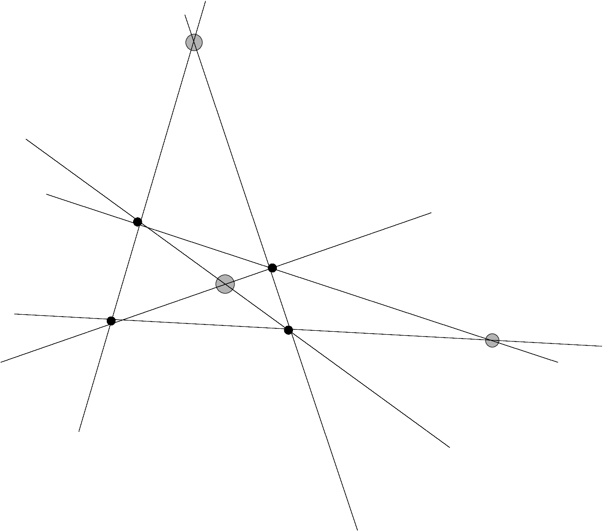
u12,34=(110),u13,24=(101),u14,23=(011).u_{12,34}=\begin{pmatrix}1\\ 1\\ 0\end{pmatrix},\ u_{13,24}=\begin{pmatrix}1\\ 0\\ 1\end{pmatrix},\ u_{14,23}=\begin{pmatrix}0\\ 1\\ 1\end{pmatrix}.
Refer to caption
Figure 9. Points and lines from the default framing of ℙ2\mathbb{P}^{2}. Original four points are black dots, three new are shaded dots

These determine further lines

v(12,34),(13,24)=(−1,1,1),v(12,34),(14,23)=(1,−1,1),v(13,24),(14,23)=(1,1,−1),v_{(12,34),(13,24)}=(-1,1,1),\ \ v_{(12,34),(14,23)}=(1,-1,1),\ \ v_{(13,24),(14,23)}=(1,1,-1),

which determine

u34,(13,24|14,23)=(112),u24,(12,34|14,23)=(121),u23,(12,34|13,24)=(211),u_{34,(13,24|14,23)}=\begin{pmatrix}1\\ 1\\ 2\end{pmatrix},\ u_{24,(12,34|14,23)}=\begin{pmatrix}1\\ 2\\ 1\end{pmatrix},\ u_{23,(12,34|13,24)}=\begin{pmatrix}2\\ 1\\ 1\end{pmatrix},
u12,(12,34|13,24)=(110),u13,(12,34|13,24)=(101),u14,(12,34|13,24)=(011).u_{12,(12,34|13,24)}=\begin{pmatrix}1\\ 1\\ 0\end{pmatrix},\ u_{13,(12,34|13,24)}=\begin{pmatrix}1\\ 0\\ 1\end{pmatrix},\ u_{14,(12,34|13,24)}=\begin{pmatrix}0\\ 1\\ 1\end{pmatrix}.

This process continues, giving rise to an infinite collection of points but in practice only vectors from the first 33 rounds appeared in decompositions.

6.2. Point-line configuration for 𝒮ℤ4×ℤ3{\mathcal{S}}_{\mathbb{Z}_{4}\times\mathbb{Z}_{3}}

The rank one elements appearing in 𝒮ℤ4×ℤ3{\mathcal{S}}_{\mathbb{Z}_{4}\times\mathbb{Z}_{3}} consist of points from three rounds of points obtained from the default configuration. All points appear except that u13|24u_{13|24} is missing (the orbit under ℤ4\mathbb{Z}_{4} of u12|34u_{12|34} is {u12|34,u14|23}\{u_{12|34},u_{14|23}\}).

Here is the decomposition 𝒮ℤ4×ℤ3{\mathcal{S}}_{\mathbb{Z}_{4}\times\mathbb{Z}_{3}} in terms of the points from §6.1:

(30) M⟨3⟩=\displaystyle M_{\langle 3\rangle}= −a0⊗​3\displaystyle-a_{0}^{{\mathord{\otimes}}3}
(31) +ℤ4⋅(u1v23)⊗​3\displaystyle+\mathbb{Z}_{4}\cdot(u_{1}v_{23})^{{\mathord{\otimes}}3}
(32) +ℤ2⋅(u2v23−u12|34v23)⊗​3\displaystyle+\mathbb{Z}_{2}\cdot(u_{2}v_{23}-u_{12|34}v_{23})^{{\mathord{\otimes}}3}
(33) +ℤ4⋅(u2v24)⊗​3\displaystyle+\mathbb{Z}_{4}\cdot(u_{2}v_{24})^{{\mathord{\otimes}}3}
(34) +ℤ3×ℤ4⋅(u2v23⊗u4v14⊗u12|34v13).\displaystyle+\mathbb{Z}_{3}\times\mathbb{Z}_{4}\cdot(u_{2}v_{23}{\mathord{\otimes}}u_{4}v_{14}{\mathord{\otimes}}u_{12|34}v_{13}).

6.3. Point-line configuration for 𝒮L​a​d−ℤ3{\mathcal{S}}_{Lad-\mathbb{Z}_{3}}

Thanks to the transpose-like symmetry, it is better to label points in the dual space by their image under transpose rather than annihilators, to make the transpose-like symmetry more transparent. Points:

u1=(100),u2=(010),u3=(001),u12=(1−10),u23=(01−1).u_{1}=\begin{pmatrix}1\\ 0\\ 0\end{pmatrix},\ u_{2}=\begin{pmatrix}0\\ 1\\ 0\end{pmatrix},\ u_{3}=\begin{pmatrix}0\\ 0\\ 1\end{pmatrix},\ u_{12}=\begin{pmatrix}1\\ -1\\ 0\end{pmatrix},\ u_{23}=\begin{pmatrix}0\\ 1\\ -1\end{pmatrix}.
v1=(1,0,0),v2=(0,1,0),v3=(0,0,1),\displaystyle v_{1}=(1,0,0),\ v_{2}=(0,1,0),\ v_{3}=(0,0,1),
v12=(1,1,0),v23=(0,1,1).\displaystyle v_{12}=(1,1,0),\ v_{23}=(0,1,1).

This collection of points has a ℤ2\mathbb{Z}_{2}-symmetry generated by τ13\tau_{13} which swaps the two lines.

Refer to caption
Figure 10. Rank one ℙ​U\mathbb{P}U-points appearing in 𝒮L​a​d−ℤ3{\mathcal{S}}_{Lad-\mathbb{Z}_{3}}

In order to express 𝒮L​a​d−ℤ3{\mathcal{S}}_{Lad-\mathbb{Z}_{3}} in terms of just these points, we write the decomposition in terms of the ℤ3⋊ℤ2ζ\mathbb{Z}_{3}\rtimes\mathbb{Z}_{2}^{\zeta}-orbits.

(35) M⟨3⟩=\displaystyle M_{\langle 3\rangle}= (u2​v2)⊗​3\displaystyle(u_{2}v_{2})^{{\mathord{\otimes}}3}
(36) +(u3​v3)⊗​3\displaystyle+(u_{3}v_{3})^{{\mathord{\otimes}}3}
(37) +(u12​v1)⊗​3\displaystyle+(u_{12}v_{1})^{{\mathord{\otimes}}3}
(38) +(u1​v12)⊗​3\displaystyle+(u_{1}v_{12})^{{\mathord{\otimes}}3}
(39) +(u2​v1−u1​v12)⊗​3\displaystyle+(u_{2}v_{1}-u_{1}v_{12})^{{\mathord{\otimes}}3}
(40) +ℤ3⋅(u1v3)⊗(u3v1)⊗(u1v1)\displaystyle+\mathbb{Z}_{3}\cdot(u_{1}v_{3}){\mathord{\otimes}}(u_{3}v_{1}){\mathord{\otimes}}(u_{1}v_{1})
(41) +ℤ3⋅(u23v1)⊗(u12v3)⊗(u23v3)\displaystyle+\mathbb{Z}_{3}\cdot(u_{23}v_{1}){\mathord{\otimes}}(u_{12}v_{3}){\mathord{\otimes}}(u_{23}v_{3})
(42) +ℤ3⋅(u3v12)⊗(u1v23)⊗(u3v23)\displaystyle+\mathbb{Z}_{3}\cdot(u_{3}v_{12}){\mathord{\otimes}}(u_{1}v_{23}){\mathord{\otimes}}(u_{3}v_{23})
(43) +ℤ3⋅(u2v3−u23v1)⊗(u1v2−u12v3)⊗(u3v2−u23v3)\displaystyle+\mathbb{Z}_{3}\cdot(u_{2}v_{3}-u_{23}v_{1}){\mathord{\otimes}}(u_{1}v_{2}-u_{12}v_{3}){\mathord{\otimes}}(u_{3}v_{2}-u_{23}v_{3})
(44) +ℤ3⋊ℤ2ζ⋅(u23v12+u2v3−u1v23)⊗(u2v3)⊗(u3v2).\displaystyle+\mathbb{Z}_{3}\rtimes\mathbb{Z}_{2}^{\zeta}\cdot(u_{23}v_{12}+u_{2}v_{3}-u_{1}v_{23}){\mathord{\otimes}}(u_{2}v_{3}){\mathord{\otimes}}(u_{3}v_{2}).

6.4. Point-line arrangement for 𝒮2​f​i​x−ℤ3{\mathcal{S}}_{2fix-\mathbb{Z}_{3}}

Despite the lack of a transpose-like symmetry, both sets of points are the 66 points corresponding to lines dual to the standard configuration of four points. Again, this illustrates how the decomposition nearly has such a symmetry, and could likely be modified to have such.

Refer to caption
Figure 11. Points from 𝒮2​f​i​x−ℤ3{\mathcal{S}}_{2fix-\mathbb{Z}_{3}} rank one matrices appearing in ℙ​U\mathbb{P}U and ℙ​U∗\mathbb{P}U^{*}, with the latter expressed as lines in ℙ​U\mathbb{P}U

7. Spaces of Γ\Gamma-invariants for various Γ\Gamma

The space of ℤ3\mathbb{Z}_{3}-invariants in A⊗​3A^{{\mathord{\otimes}}3} is S3​A⊕Λ3​AS^{3}A\oplus\Lambda^{3}A. To see this, as a G​L​(A)×𝔖3GL(A)\times\mathfrak{S}_{3}-module we have the decomposition A⊗​3=S3​A​⊗​[3]⊕S21​A​⊗​[21]⊕Λ3​A​⊗​[111]A^{{\mathord{\otimes}}3}=S^{3}A{\mathord{\otimes}}[3]\oplus S_{21}A{\mathord{\otimes}}[21]\oplus\Lambda^{3}A{\mathord{\otimes}}[111]. Then ℤ3\mathbb{Z}_{3} acts trivially on the trivial representation [3][3] and trivially on the sign representation [111][111] (as the three cycle is even), and [21][21] decomposes into its e2​π​i3,e4​π​i3e^{\frac{2\pi i}{3}},e^{\frac{4\pi i}{3}} eigenspaces under ℤ3\mathbb{Z}_{3}. Thus, if dim⁡A=m\operatorname{dim}A=m, the space of invariants (A⊗​3)ℤ3(A^{{\mathord{\otimes}}3})^{\mathbb{Z}_{3}} has dimension 13​(m3+2​m)\frac{1}{3}(m^{3}+2m), so restricting the search to ℤ3\mathbb{Z}_{3}-invariant decompositions reduces the search size by about a factor of 33. (In our case, m=n2m=n^{2}.)

The ℤ3\mathbb{Z}_{3}-fixed triples all lie in S3​AS^{3}A, so one cannot have all terms of a decomposition individually ℤ3\mathbb{Z}_{3}-fixed. A-priori there could be 2+3​k2+3k ℤ3\mathbb{Z}_{3}-fixed points for 0≤k<70\leq k<7. We found decompositions with 2,52,5, and 1111 ℤ3\mathbb{Z}_{3}-fixed points, i.e., k=0,1,3k=0,1,3.

7.1. ℤn+1\mathbb{Z}_{n+1}-invariants

Consider the diagonal ℤn+1⊂P​G​Ln⊂P​G​Ln×3\mathbb{Z}_{n+1}\subset PGL_{n}\subset PGL_{n}^{\times 3} invariants: Each of U∗,VU^{*},V decomposes into nn one-dimensional representations for ℤn+1\mathbb{Z}_{n+1}, corresponding to the eigenvalues ω,ω2,…,ωn\omega,\omega^{2},\ldots,\omega^{n} where ω=e2​π​in+1\omega=e^{\frac{2\pi i}{n+1}}. Write (U∗)j,Vj(U^{*})_{j},V_{j} for the eigenspace corresponding to ωj\omega^{j}. Then, adding indices modulo n+1n+1, and letting u∈[n]u\in[n],

A0=⨁t=1nUt∗​⊗​Vn+1−t,\displaystyle A_{0}=\bigoplus_{t=1}^{n}U^{*}_{t}{\mathord{\otimes}}V_{n+1-t},
Au=⨁i=1,i≠unUi∗​⊗​Vu−i,\displaystyle A_{u}=\bigoplus_{i=1,i\neq u}^{n}U^{*}_{i}{\mathord{\otimes}}V_{u-i},

so dim⁡A0=n\operatorname{dim}A_{0}=n, and dim⁡Au=n−1\operatorname{dim}A_{u}=n-1, where each AiA_{i} is a ℤn+1\mathbb{Z}_{n+1}-isotypic component of AA. Note that A0A_{0} is spanned by the powers of a0a_{0} of (1).

The space of ℤn+1\mathbb{Z}_{n+1} invariants in A​⊗​B​⊗​CA{\mathord{\otimes}}B{\mathord{\otimes}}C is spanned by the spaces Aα​⊗​Bβ​⊗​CγA_{\alpha}{\mathord{\otimes}}B_{\beta}{\mathord{\otimes}}C_{\gamma} with α+β+γ≡0​mod⁡n+1\alpha+\beta+\gamma\equiv 0\operatorname{mod}n+1. Let 1≤i,j≤n1\leq i,j\leq n, we have the following dimensions:

space dimension number of such total contribution
A0​⊗​B0​⊗​C0A_{0}{\mathord{\otimes}}B_{0}{\mathord{\otimes}}C_{0} n3n^{3} 11 n3n^{3}
A0​⊗​Bj​⊗​Cn+1−jA_{0}{\mathord{\otimes}}B_{j}{\mathord{\otimes}}C_{n+1-j} plus cyclic perms n​(n−1)2n(n-1)^{2} 3​n3n 3​n2​(n−1)23n^{2}(n-1)^{2}
Ai​⊗​Bj​⊗​Cn+1−j−iA_{i}{\mathord{\otimes}}B_{j}{\mathord{\otimes}}C_{n+1-j-i}, i+j≠n+1i+j\neq n+1 (n−1)3(n-1)^{3} n⁡(n−1)n(n-1) n​(n−1)4n(n-1)^{4}

Thus

Proposition 7.1.

The space of ℤn+1⊂P​G​Ln⊂P​G​Ln×3\mathbb{Z}_{n+1}\subset PGL_{n}\subset PGL_{n}^{\times 3} invariants for the diagonal ℤn+1\mathbb{Z}_{n+1} in ℂn2​⊗​ℂn2​⊗​ℂn2\mathbb{C}^{n^{2}}{\mathord{\otimes}}\mathbb{C}^{n^{2}}{\mathord{\otimes}}\mathbb{C}^{n^{2}} is n5−n4+n3−n2+nn^{5}-n^{4}+n^{3}-n^{2}+n. In particular, when n=2,3,4n=2,3,4 these dimensions are respectively 22,183,82022,183,820.

7.2. ℤn+1×ℤ3\mathbb{Z}_{n+1}\times\mathbb{Z}_{3}-invariants

We look inside S3​A⊕Λ3​AS^{3}A\oplus\Lambda^{3}A for ℤn+1\mathbb{Z}_{n+1}-invariants. Write

S3​A\displaystyle S^{3}A =S3(A0+⋯+An)=S3A0⊕⨁j=1nS3Aj⊕⨁j=1nA0⊗S2Aj⊕⨁j=1nAj⊗S2A0\displaystyle=S^{3}(A_{0}+\cdots+A_{n})=S^{3}A_{0}\quad\oplus\quad\bigoplus_{j=1}^{n}S^{3}A_{j}\quad\oplus\quad\bigoplus_{j=1}^{n}A_{0}{\mathord{\otimes}}S^{2}A_{j}\quad\oplus\quad\bigoplus_{j=1}^{n}A_{j}{\mathord{\otimes}}S^{2}A_{0}
⊕⨁j,k=1,j≠knAj​⊗​S2​Ak⊕⨁1≤j<k≤nA0​⊗​Aj⊗Ak⊕⨁1≤i<j<k≤nAi​⊗​Aj​⊗​Ak.\displaystyle\oplus\quad\bigoplus_{j,k=1,j\neq k}^{n}A_{j}{\mathord{\otimes}}S^{2}A_{k}\quad\oplus\quad\bigoplus_{1\leq j<k\leq n}A_{0}{\mathord{\otimes}}A_{j}\otimes A_{k}\quad\oplus\quad\bigoplus_{1\leq i<j<k\leq n}A_{i}{\mathord{\otimes}}A_{j}{\mathord{\otimes}}A_{k}.

The subspace of ℤn+1\mathbb{Z}_{n+1}-invariants is (here all indices run from 11 to nn)

(S3​A)ℤn+1=S3​A0⊕⨁j| 3​j≡0​mod⁡n+1S3​Aj⊕⨁j| 2​j≡0​mod⁡n+1A0​⊗​S2​Aj⊕0\displaystyle(S^{3}A)^{\mathbb{Z}_{n+1}}=S^{3}A_{0}\quad\oplus\quad\bigoplus_{j\mid\,3j\equiv 0\operatorname{mod}n+1}S^{3}A_{j}\quad\oplus\quad\bigoplus_{j\mid\,2j\equiv 0\operatorname{mod}n+1}A_{0}{\mathord{\otimes}}S^{2}A_{j}\quad\oplus\quad 0
⊕⨁(j,k)∣j+2k≡0modn+1;j≠kAj⊗S2Ak⊕⨁i|i<n+1−iA0⊗Ai⊗An+1−i⊕⨁(i,j)|i<j<n+1−i−j or ​i<j<2​n+2−i−j<n+1Ai⊗Aj⊗An+1−i−j.\displaystyle\oplus\bigoplus_{(j,k)\mid\,j+2k\equiv 0\operatorname{mod}n+1;j\neq k}A_{j}{\mathord{\otimes}}S^{2}A_{k}\quad\oplus\quad\bigoplus_{i\mid\,i<n+1-i}A_{0}{\mathord{\otimes}}A_{i}{\mathord{\otimes}}A_{n+1-i}\quad\oplus\quad\bigoplus_{(i,j)\mid\,i<j<n+1-i-j\atop\text{ or }i<j<2n+2-i-j<n+1}A_{i}{\mathord{\otimes}}A_{j}{\mathord{\otimes}}A_{n+1-i-j}.

The dimensions of the summands of the various types are respectively

(n+23),(n+13),n​(n2), 0,(n−1)​(n2),n​(n−1)2,(n−1)3.\binom{n+2}{3},\ \binom{n+1}{3},\ n\binom{n}{2},\ 0,\ (n-1)\binom{n}{2},\ n(n-1)^{2},\ (n-1)^{3}.

Similarly, the space of ℤn+1\mathbb{Z}_{n+1}-invariants in Λ3​A\Lambda^{3}A is

(Λ3​A)ℤn+1=\displaystyle(\Lambda^{3}A)^{\mathbb{Z}_{n+1}}= Λ3​A0⊕⨁j| 3​j≡0​mod⁡n+1Λ3​Aj⊕⨁j| 2​j≡0​mod⁡n+1A0​⊗​Λ2​Aj⊕0\displaystyle\Lambda^{3}A_{0}\oplus\bigoplus_{j\mid\,3j\equiv 0\operatorname{mod}n+1}\Lambda^{3}A_{j}\oplus\bigoplus_{j\mid\,2j\equiv 0\operatorname{mod}n+1}A_{0}{\mathord{\otimes}}\Lambda^{2}A_{j}\oplus 0
⊕⨁(i,j)∣i+2j≡0modn+1;i≠jAi⊗Λ2Aj⊕⨁i|i<n+1−iA0⊗Ai⊗An+1−i⊕⨁(i,j)|i<j<n+1−i−j or ​i<j<2​n+2−i−j<n+1Ai⊗Aj⊗An+1−i−j.\displaystyle\oplus\bigoplus_{(i,j)\mid\,i+2j\equiv 0\operatorname{mod}n+1;i\neq j}A_{i}{\mathord{\otimes}}\Lambda^{2}A_{j}\oplus\bigoplus_{i\mid\,i<n+1-i}A_{0}{\mathord{\otimes}}A_{i}{\mathord{\otimes}}A_{n+1-i}\oplus\bigoplus_{(i,j)\mid\,i<j<n+1-i-j\atop\text{ or }i<j<2n+2-i-j<n+1}A_{i}{\mathord{\otimes}}A_{j}{\mathord{\otimes}}A_{n+1-i-j}.

The dimensions of the summands of the various types are respectively

(n3),(n−13),n​(n−12), 0,(n−1)​(n−12),n​(n−1)2,(n−1)3.\binom{n}{3},\ \binom{n-1}{3},\ n\binom{n-1}{2},\ 0,\ (n-1)\binom{n-1}{2},\ n(n-1)^{2},\ (n-1)^{3}.

In both cases, the number of terms of each type depends on divisibility properties of nn. When n=2n=2, the summands are

S3​A0⊕S3​A1⊕S3​A2⊕(A0​⊗​A1​⊗​A2)S⊕(A0​⊗​A1​⊗​A2)Λ,S^{3}A_{0}\oplus S^{3}A_{1}\oplus S^{3}A_{2}\oplus(A_{0}{\mathord{\otimes}}A_{1}{\mathord{\otimes}}A_{2})^{S}\oplus(A_{0}{\mathord{\otimes}}A_{1}{\mathord{\otimes}}A_{2})^{\Lambda},

for a total dimension of 8+2=108+2=10. (Here the S,ΛS,\Lambda superscripts are whether the factor is in S3S^{3} or Λ3\Lambda^{3}.)

When n=3n=3, the summands are

S3​A0⊕A0​⊗​S2​A2⊕A2​⊗​S2​A1⊕A2​⊗​S2​A3⊕(A0​⊗​A1​⊗​A3)S\displaystyle S^{3}A_{0}\oplus A_{0}{\mathord{\otimes}}S^{2}A_{2}\oplus A_{2}{\mathord{\otimes}}S^{2}A_{1}\oplus A_{2}{\mathord{\otimes}}S^{2}A_{3}\oplus(A_{0}{\mathord{\otimes}}A_{1}{\mathord{\otimes}}A_{3})^{S}
⊕Λ3​A0⊕A0​⊗​Λ2​A2⊕A2​⊗​Λ2​A1⊕A2​⊗​Λ2​A3⊕(A0​⊗​A1​⊗​A3)Λ,\displaystyle\oplus\Lambda^{3}A_{0}\oplus A_{0}{\mathord{\otimes}}\Lambda^{2}A_{2}\oplus A_{2}{\mathord{\otimes}}\Lambda^{2}A_{1}\oplus A_{2}{\mathord{\otimes}}\Lambda^{2}A_{3}\oplus(A_{0}{\mathord{\otimes}}A_{1}{\mathord{\otimes}}A_{3})^{\Lambda},

for a total dimension of 43+20=6343+20=63.

M⟨3⟩M_{\langle 3\rangle} has a nonzero projection onto each factor except the one-dimensional Λ3​A0\Lambda^{3}A_{0}.

When n=4n=4 the summands are

S3​A0⊕A1​⊗​S2​A2⊕A2​⊗​S2​A4⊕A3​⊗​S2​A1⊕A4​⊗​S2​A3⊕(A0​⊗​A1​⊗​A4)S⊕(A0​⊗​A2​⊗​A3)S\displaystyle S^{3}A_{0}\oplus A_{1}{\mathord{\otimes}}S^{2}A_{2}\oplus A_{2}{\mathord{\otimes}}S^{2}A_{4}\oplus A_{3}{\mathord{\otimes}}S^{2}A_{1}\oplus A_{4}{\mathord{\otimes}}S^{2}A_{3}\oplus(A_{0}{\mathord{\otimes}}A_{1}{\mathord{\otimes}}A_{4})^{S}\oplus(A_{0}{\mathord{\otimes}}A_{2}{\mathord{\otimes}}A_{3})^{S}
⊕Λ3​A0⊕A1​⊗​Λ2​A3⊕A2⊕Λ2​A4​⊗​A3​⊗​Λ2​A1⊕A4​⊗​Λ2​A3⊕(A0​⊗​A1​⊗​A4)Λ⊕(A0​⊗​A2​⊗​A3)Λ,\displaystyle\oplus\Lambda^{3}A_{0}\oplus A_{1}{\mathord{\otimes}}\Lambda^{2}A_{3}\oplus A_{2}\oplus\Lambda^{2}A_{4}{\mathord{\otimes}}A_{3}{\mathord{\otimes}}\Lambda^{2}A_{1}\oplus A_{4}{\mathord{\otimes}}\Lambda^{2}A_{3}\oplus(A_{0}{\mathord{\otimes}}A_{1}{\mathord{\otimes}}A_{4})^{\Lambda}\oplus(A_{0}{\mathord{\otimes}}A_{2}{\mathord{\otimes}}A_{3})^{\Lambda},

for a total dimension of 164+112=276164+112=276, compared with the naïve search space dimension of 163=409616^{3}=4096 and the ℤ3\mathbb{Z}_{3}-invariant search space of dimension 13761376.

In summary:

Proposition 7.2.

The dimension of the space of ℤn+1×ℤ3\mathbb{Z}_{n+1}\times\mathbb{Z}_{3} invariants in (U∗​⊗​U)⊗​3(U^{*}{\mathord{\otimes}}U)^{{\mathord{\otimes}}3} is respectively of dimensions 1010, 6363, and 276276 when n=2,3,4n=2,3,4.

8. Eigenvalues

When we deal with a restricted family P​G​Ln⋅𝒮PGL_{n}\cdot{\mathcal{S}}, it makes sense to discuss eigenlines and eigenvalues of the terms appearing. These also facilitate determining if two decompositions lie in the same family, beyond the graphs.

𝒮ℤ4×ℤ3{\mathcal{S}}_{\mathbb{Z}_{4}\times\mathbb{Z}_{3}} Char. Poly. Count
symmetric t2​(t−1)t^{2}(t-1) 6
t+t2+t3t+t^{2}+t^{3} 4
t−t2+t3−1t-t^{2}+t^{3}-1 1
triples {t3,t3,t3}\left\{t^{3},t^{3},t^{3}\right\} 4
Table 1. Characteristic polynomials of matrices appearing in 𝒮ℤ4×ℤ3{\mathcal{S}}_{\mathbb{Z}_{4}\times\mathbb{Z}_{3}}
𝒮L​a​d​e​r−ℤ3{\mathcal{S}}_{Lader-\mathbb{Z}_{3}} Char. Poly. Count
symmetric t2​(t−1)t^{2}(t-1) 4
t+t2+t3t+t^{2}+t^{3} 1
triples {t2​(t−1),t3,t3}\left\{t^{2}(t-1),t^{3},t^{3}\right\} 3
{t3,t3,t+t2+t3}\left\{t^{3},t^{3},t+t^{2}+t^{3}\right\} 1
{t3,t3,t−t2+t3−1}\left\{t^{3},t^{3},t-t^{2}+t^{3}-1\right\} 2
Table 2. Characteristic polynomials of matrices appearing in 𝒮L​a​d​e​r−ℤ3{\mathcal{S}}_{Lader-\mathbb{Z}_{3}}
𝒮2​f​i​x−ℤ3{\mathcal{S}}_{2fix-\mathbb{Z}_{3}} Char. Poly. Count
symmetric t​(t−1)2t(t-1)^{2} 1
t2​(t−1)t^{2}(t-1) 1
triples {t3,t3,t3}\left\{t^{3},t^{3},t^{3}\right\} 1
{t2​(t−1),t2​(t−1),t+t2+t3}\left\{t^{2}(t-1),t^{2}(t-1),t+t^{2}+t^{3}\right\} 1
{t2​(t−1),t3,t3}\left\{t^{2}(t-1),t^{3},t^{3}\right\} 2
{t2​(t−1),t2​(t−1),t3}\left\{t^{2}(t-1),t^{2}(t-1),t^{3}\right\} 2
{t2​(t−1),t2​(t−1),t2​(t+1)}\left\{t^{2}(t-1),t^{2}(t-1),t^{2}(t+1)\right\} 1
Table 3. Characteristic polynomials of matrices appearing in 𝒮2​f​i​x−ℤ3{\mathcal{S}}_{2fix-\mathbb{Z}_{3}}

References

  • [1] Austin R. Benson and Grey Ballard, A framework for practical parallel fast matrix multiplication, Proceedings of the 20th ACM SIGPLAN Symposium on Principles and Practice of Parallel Programming (New York, NY, USA), PPoPP 2015, ACM, February 2015, pp. 42–53.
  • [2] Jerome Brachat, Pierre Comon, Bernard Mourrain, and Elias Tsigaridas, Symmetric tensor decomposition, Linear Algebra Appl. 433 (2010), no. 11-12, 1851–1872. MR 2736103
  • [3] Jaroslaw Buczyński, Adam Ginensky, and J. M. Landsberg, Determinantal equations for secant varieties and the Eisenbud-Koh-Stillman conjecture, J. Lond. Math. Soc. (2) 88 (2013), no. 1, 1–24. MR 3092255
  • [4] Vladimir P. Burichenko, On symmetries of the strassen algorithm, CoRR abs/1408.6273 (2014).
  • [5] by same author, Symmetries of matrix multiplication algorithms. I, CoRR abs/1508.01110 (2015).
  • [6] Luca Chiantini, Christian Ikenmeyer, J. M. Landsberg, and Giorgio Ottaviani, The geometry of rank decompositions of matrix multiplication I: 2x2 matrices, CoRR abs/1610.08364 (2016).
  • [7] Hans F. de Groote, On varieties of optimal algorithms for the computation of bilinear mappings. I. The isotropy group of a bilinear mapping, Theoret. Comput. Sci. 7 (1978), no. 1, 1–24. MR 0506377
  • [8] by same author, On varieties of optimal algorithms for the computation of bilinear mappings. II. Optimal algorithms for 2×22\times 2-matrix multiplication, Theoret. Comput. Sci. 7 (1978), no. 2, 127–148. MR 509013 (81i:68061)
  • [9] Robert Fourer, David M. Gay, and Brian W. Kernighan, Ampl: A modeling language for mathematical programming, second ed., 2002.
  • [10] Shmuel Friedland, Remarks on the symmetric rank of symmetric tensors, SIAM J. Matrix Anal. Appl. 37 (2016), no. 1, 320–337. MR 3474849
  • [11] Fulvio Gesmundo, Geometric aspects of iterated matrix multiplication, J. Algebra 461 (2016), 42–64. MR 3513064
  • [12] J. A. Grochow and C. Moore, Matrix multiplication algorithms from group orbits, ArXiv e-prints (2016).
  • [13] Rodney W. Johnson and Aileen M. McLoughlin, Noncommutative bilinear algorithms for 3×33\times 3 matrix multiplication, SIAM J. Comput. 15 (1986), no. 2, 595–603. MR 837607
  • [14] T. G. Kolda and B. W. Bader, Tensor decompositions and applications, SIAM Review 51 (2009), no. 3, 455–500.
  • [15] Julian D. Laderman, A noncommutative algorithm for multiplying 3×33\times 3 matrices using 2323 muliplications, Bull. Amer. Math. Soc. 82 (1976), no. 1, 126–128. MR MR0395320 (52 #16117)
  • [16] J. M. Landsberg, Geometry and complexity theory, Cambridge Studies in Advanced Mathematics, Cambridge University Press, 2017.
  • [17] J. M. Landsberg and Mateusz Michalek, On the geometry of border rank decompositions for matrix multiplication and other tensors with symmetry, SIAM J. Appl. Algebra Geom. 1 (2017), no. 1, 2–19. MR 3633766
  • [18] J.M. Landsberg and Nicolas Ressayre, Permanent v. determinant: an exponential lower bound assuming symmetry and a potential path towards valiant’s conjecture, arXiv:1508.05788 (2015).
  • [19] Hwangrae Lee, Power sum decompositions of elementary symmetric polynomials, Linear Algebra Appl. 492 (2016), 89–97. MR 3440150
  • [20] A. Sedoglavic, Laderman matrix multiplication algorithm can be constructed using Strassen algorithm and related tensor’s isotropies, ArXiv e-prints (2017).
  • [21] Y. Shitov, A counterexample to Comon’s conjecture, ArXiv e-prints (2017).
  • [22] A.V. Smirnov, The bilinear complexity and practical algorithms for matrix multiplication, Computational Mathematics and Mathematical Physics 53 (2013), no. 12, 1781–1795 (English).
  • [23] Robert J Vanderbei, LOQO user’s manual-version 3.10, Optimization methods and software 11 (1999), no. 1-4, 485–514.

Appendix A Additional decompositions

What follows are three additional decompositions with their graphs and eigenvalue tables.

A.1. A decomposition with five ℤ3\mathbb{Z}_{3}-fixed points and no diagonal G​L3GL_{3}-symmetry

The lack of extra symmetry may be easily deduced from the incidence graph.

(45) M⟨3⟩\displaystyle M_{\langle 3\rangle} =(0000000−11)⊗​3+(100100000)⊗​3+(1−100000−10)⊗​3\displaystyle=\begin{pmatrix}0&0&0\\ 0&0&0\\ 0&-1&1\end{pmatrix}^{{\mathord{\otimes}}3}+\begin{pmatrix}1&0&0\\ 1&0&0\\ 0&0&0\end{pmatrix}^{{\mathord{\otimes}}3}+\begin{pmatrix}1&-1&0\\ 0&0&0\\ 0&-1&0\end{pmatrix}^{{\mathord{\otimes}}3}
(46) +(000010010)⊗​3+(−110−100010)⊗​3\displaystyle+\begin{pmatrix}0&0&0\\ 0&1&0\\ 0&1&0\end{pmatrix}^{{\mathord{\otimes}}3}+\begin{pmatrix}-1&1&0\\ -1&0&0\\ 0&1&0\end{pmatrix}^{{\mathord{\otimes}}3}
(47) +ℤ3s​t​d⋅(000001000)⊗(000000−100)⊗(0−11000000)\displaystyle+\mathbb{Z}_{3}^{std}\cdot\begin{pmatrix}0&0&0\\ 0&0&1\\ 0&0&0\end{pmatrix}{\mathord{\otimes}}\begin{pmatrix}0&0&0\\ 0&0&0\\ -1&0&0\end{pmatrix}{\mathord{\otimes}}\begin{pmatrix}0&-1&1\\ 0&0&0\\ 0&0&0\end{pmatrix}
(48) +ℤ3s​t​d⋅(0000−110−11)⊗(10−1−1−110−10)⊗(0000000−10)\displaystyle+\mathbb{Z}_{3}^{std}\cdot\begin{pmatrix}0&0&0\\ 0&-1&1\\ 0&-1&1\end{pmatrix}{\mathord{\otimes}}\begin{pmatrix}1&0&-1\\ -1&-1&1\\ 0&-1&0\end{pmatrix}{\mathord{\otimes}}\begin{pmatrix}0&0&0\\ 0&0&0\\ 0&-1&0\end{pmatrix}
(49) +ℤ3s​t​d⋅(00011−111−1)⊗(−101000000)⊗(000001001)\displaystyle+\mathbb{Z}_{3}^{std}\cdot\begin{pmatrix}0&0&0\\ 1&1&-1\\ 1&1&-1\end{pmatrix}{\mathord{\otimes}}\begin{pmatrix}-1&0&1\\ 0&0&0\\ 0&0&0\end{pmatrix}{\mathord{\otimes}}\begin{pmatrix}0&0&0\\ 0&0&1\\ 0&0&1\end{pmatrix}
(50) +ℤ3s​t​d⋅(0000010−11)⊗(00011−101−1)⊗(10−10000−10)\displaystyle+\mathbb{Z}_{3}^{std}\cdot\begin{pmatrix}0&0&0\\ 0&0&1\\ 0&-1&1\end{pmatrix}{\mathord{\otimes}}\begin{pmatrix}0&0&0\\ 1&1&-1\\ 0&1&-1\end{pmatrix}{\mathord{\otimes}}\begin{pmatrix}1&0&-1\\ 0&0&0\\ 0&-1&0\end{pmatrix}
(51) +ℤ3s​t​d⋅(000000100)⊗(100000000)⊗(001001001)\displaystyle+\mathbb{Z}_{3}^{std}\cdot\begin{pmatrix}0&0&0\\ 0&0&0\\ 1&0&0\end{pmatrix}{\mathord{\otimes}}\begin{pmatrix}1&0&0\\ 0&0&0\\ 0&0&0\end{pmatrix}{\mathord{\otimes}}\begin{pmatrix}0&0&1\\ 0&0&1\\ 0&0&1\end{pmatrix}
(52) +ℤ3s​t​d⋅(0−100000−10)⊗(1−101−100−10)⊗(000100000)\displaystyle+\mathbb{Z}_{3}^{std}\cdot\begin{pmatrix}0&-1&0\\ 0&0&0\\ 0&-1&0\end{pmatrix}{\mathord{\otimes}}\begin{pmatrix}1&-1&0\\ 1&-1&0\\ 0&-1&0\end{pmatrix}{\mathord{\otimes}}\begin{pmatrix}0&0&0\\ 1&0&0\\ 0&0&0\end{pmatrix}
001\begin{matrix}0&0&1\end{matrix} 4 011\begin{matrix}0&1&1\end{matrix} 4 100\begin{matrix}1&0&0\end{matrix} 3 010\begin{matrix}0&1&0\end{matrix} 2 110\begin{matrix}1&1&0\end{matrix} 1 101\begin{matrix}1&0&1\end{matrix} 1 111\begin{matrix}1&1&1\end{matrix} 1 100\begin{matrix}1&0&0\end{matrix} 5 010\begin{matrix}0&1&0\end{matrix} 3 001\begin{matrix}0&0&1\end{matrix} 3 01−1\begin{matrix}0&1&-1\end{matrix} 3 10−1\begin{matrix}1&0&-1\end{matrix} 1 11−1\begin{matrix}1&1&-1\end{matrix} 1
Figure 12. Incidence graph of Addtl. Dec. #1
001\begin{matrix}0&0&1\end{matrix} 4 011\begin{matrix}0&1&1\end{matrix} 4 100\begin{matrix}1&0&0\end{matrix} 3 010\begin{matrix}0&1&0\end{matrix} 2 110\begin{matrix}1&1&0\end{matrix} 1 101\begin{matrix}1&0&1\end{matrix} 1 111\begin{matrix}1&1&1\end{matrix} 1 100\begin{matrix}1&0&0\end{matrix} 5 010\begin{matrix}0&1&0\end{matrix} 3 001\begin{matrix}0&0&1\end{matrix} 3 01−1\begin{matrix}0&1&-1\end{matrix} 3 10−1\begin{matrix}1&0&-1\end{matrix} 1 11−1\begin{matrix}1&1&-1\end{matrix} 1
Figure 13. Pairing graph of Addtl. Dec. #1
Addtl. Dec. #1 Char. Poly. Count
symmetric t2​(t−1)t^{2}(t-1) 4
t+t2+t3t+t^{2}+t^{3} 1
triples {t3,t3,t3}\left\{t^{3},t^{3},t^{3}\right\} 3
{t2​(t−1),t2​(t+1),t3}\left\{t^{2}(t-1),t^{2}(t+1),t^{3}\right\} 1
{t2​(t−1),t3,t−t2+t3}\left\{t^{2}(t-1),t^{3},t-t^{2}+t^{3}\right\} 1
{t2​(t−1),t2​(t−1),t3}\left\{t^{2}(t-1),t^{2}(t-1),t^{3}\right\} 1
Table 4. Characteristic polynomials of matrices appearing in Addtl. Dec. #1

A.2. Another decomposition with five ℤ3\mathbb{Z}_{3}-fixed points

(53) M⟨3⟩\displaystyle M_{\langle 3\rangle} =(01−1010000)⊗​3+(000−111000)⊗​3+(100000000)⊗​3\displaystyle=\begin{pmatrix}0&1&-1\\ 0&1&0\\ 0&0&0\end{pmatrix}^{{\mathord{\otimes}}3}+\begin{pmatrix}0&0&0\\ -1&1&1\\ 0&0&0\end{pmatrix}^{{\mathord{\otimes}}3}+\begin{pmatrix}1&0&0\\ 0&0&0\\ 0&0&0\end{pmatrix}^{{\mathord{\otimes}}3}
(54) +(0−111−1−1000)⊗​3+(000000001)⊗​3\displaystyle+\begin{pmatrix}0&-1&1\\ 1&-1&-1\\ 0&0&0\end{pmatrix}^{{\mathord{\otimes}}3}+\begin{pmatrix}0&0&0\\ 0&0&0\\ 0&0&1\end{pmatrix}^{{\mathord{\otimes}}3}
(55) +ℤ3s​t​d⋅(−101000−101)⊗(000010010)⊗(000001000)\displaystyle+\mathbb{Z}_{3}^{std}\cdot\begin{pmatrix}-1&0&1\\ 0&0&0\\ -1&0&1\end{pmatrix}{\mathord{\otimes}}\begin{pmatrix}0&0&0\\ 0&1&0\\ 0&1&0\end{pmatrix}{\mathord{\otimes}}\begin{pmatrix}0&0&0\\ 0&0&1\\ 0&0&0\end{pmatrix}
(56) +ℤ3s​t​d⋅(0−11000000)⊗(000−101000)⊗(1−101−1−1000)\displaystyle+\mathbb{Z}_{3}^{std}\cdot\begin{pmatrix}0&-1&1\\ 0&0&0\\ 0&0&0\end{pmatrix}{\mathord{\otimes}}\begin{pmatrix}0&0&0\\ -1&0&1\\ 0&0&0\end{pmatrix}{\mathord{\otimes}}\begin{pmatrix}1&-1&0\\ 1&-1&-1\\ 0&0&0\end{pmatrix}
(57) +ℤ3s​t​d⋅(000100100)⊗(−100000−100)⊗(0−100−100−10)\displaystyle+\mathbb{Z}_{3}^{std}\cdot\begin{pmatrix}0&0&0\\ 1&0&0\\ 1&0&0\end{pmatrix}{\mathord{\otimes}}\begin{pmatrix}-1&0&0\\ 0&0&0\\ -1&0&0\end{pmatrix}{\mathord{\otimes}}\begin{pmatrix}0&-1&0\\ 0&-1&0\\ 0&-1&0\end{pmatrix}
(58) +ℤ3s​t​d⋅(00000−1000)⊗(01−100001−1)⊗(0000−10000)\displaystyle+\mathbb{Z}_{3}^{std}\cdot\begin{pmatrix}0&0&0\\ 0&0&-1\\ 0&0&0\end{pmatrix}{\mathord{\otimes}}\begin{pmatrix}0&1&-1\\ 0&0&0\\ 0&1&-1\end{pmatrix}{\mathord{\otimes}}\begin{pmatrix}0&0&0\\ 0&-1&0\\ 0&0&0\end{pmatrix}
(59) +ℤ3s​t​d⋅(10−1000100)⊗(01−1010010)⊗(000−101−100)\displaystyle+\mathbb{Z}_{3}^{std}\cdot\begin{pmatrix}1&0&-1\\ 0&0&0\\ 1&0&0\end{pmatrix}{\mathord{\otimes}}\begin{pmatrix}0&1&-1\\ 0&1&0\\ 0&1&0\end{pmatrix}{\mathord{\otimes}}\begin{pmatrix}0&0&0\\ -1&0&1\\ -1&0&0\end{pmatrix}
(60) +ℤ3s​t​d⋅(0−11−1−11−1−11)⊗(000000−100)⊗(00−1000000)\displaystyle+\mathbb{Z}_{3}^{std}\cdot\begin{pmatrix}0&-1&1\\ -1&-1&1\\ -1&-1&1\end{pmatrix}{\mathord{\otimes}}\begin{pmatrix}0&0&0\\ 0&0&0\\ -1&0&0\end{pmatrix}{\mathord{\otimes}}\begin{pmatrix}0&0&-1\\ 0&0&0\\ 0&0&0\end{pmatrix}
010\begin{matrix}0&1&0\end{matrix} 5 100\begin{matrix}1&0&0\end{matrix} 3 101\begin{matrix}1&0&1\end{matrix} 3 001\begin{matrix}0&0&1\end{matrix} 2 011\begin{matrix}0&1&1\end{matrix} 2 111\begin{matrix}1&1&1\end{matrix} 1 100\begin{matrix}1&0&0\end{matrix} 4 001\begin{matrix}0&0&1\end{matrix} 4 010\begin{matrix}0&1&0\end{matrix} 3 10−1\begin{matrix}1&0&-1\end{matrix} 2 01−1\begin{matrix}0&1&-1\end{matrix} 2 −111\begin{matrix}-1&1&1\end{matrix} 1
Figure 14. Incidence graph of Addtl. Dec. #2
010\begin{matrix}0&1&0\end{matrix} 5 100\begin{matrix}1&0&0\end{matrix} 3 101\begin{matrix}1&0&1\end{matrix} 3 001\begin{matrix}0&0&1\end{matrix} 2 011\begin{matrix}0&1&1\end{matrix} 2 111\begin{matrix}1&1&1\end{matrix} 1 100\begin{matrix}1&0&0\end{matrix} 4 001\begin{matrix}0&0&1\end{matrix} 4 010\begin{matrix}0&1&0\end{matrix} 3 10−1\begin{matrix}1&0&-1\end{matrix} 2 01−1\begin{matrix}0&1&-1\end{matrix} 2 −111\begin{matrix}-1&1&1\end{matrix} 1
Figure 15. Pairing graph of Addtl. Dec. #2
Addtl. Dec. #2 Char. Poly. Count
symmetric t2​(t−1)t^{2}(t-1) 4
t+t2+t3t+t^{2}+t^{3} 1
triples {t2​(t−1),t3,t3}\left\{t^{2}(t-1),t^{3},t^{3}\right\} 1
{t3,t3,t3}\left\{t^{3},t^{3},t^{3}\right\} 2
{t2​(t+1),t2​(t+1),t3}\left\{t^{2}(t+1),t^{2}(t+1),t^{3}\right\} 2
{t2​(t−1),t3,t−t2+t3}\left\{t^{2}(t-1),t^{3},t-t^{2}+t^{3}\right\} 1
Table 5. Characteristic polynomials of matrices appearing in Addtl. Dec. #2

A.3. Another decomposition with 22 ℤ3\mathbb{Z}_{3}-fixed points

(61) M⟨3⟩\displaystyle M_{\langle 3\rangle} =(000010001)⊗​3+(100000000)⊗​3\displaystyle=\begin{pmatrix}0&0&0\\ 0&1&0\\ 0&0&1\end{pmatrix}^{{\mathord{\otimes}}3}+\begin{pmatrix}1&0&0\\ 0&0&0\\ 0&0&0\end{pmatrix}^{{\mathord{\otimes}}3}
(62) +ℤ3s​t​d⋅(000000001)⊗(0000−10010)⊗(000011000)\displaystyle+\mathbb{Z}_{3}^{std}\cdot\begin{pmatrix}0&0&0\\ 0&0&0\\ 0&0&1\end{pmatrix}{\mathord{\otimes}}\begin{pmatrix}0&0&0\\ 0&-1&0\\ 0&1&0\end{pmatrix}{\mathord{\otimes}}\begin{pmatrix}0&0&0\\ 0&1&1\\ 0&0&0\end{pmatrix}
(63) +ℤ3s​t​d⋅(000110000)⊗(−10−1000000)⊗(0−10000000)\displaystyle+\mathbb{Z}_{3}^{std}\cdot\begin{pmatrix}0&0&0\\ 1&1&0\\ 0&0&0\end{pmatrix}{\mathord{\otimes}}\begin{pmatrix}-1&0&-1\\ 0&0&0\\ 0&0&0\end{pmatrix}{\mathord{\otimes}}\begin{pmatrix}0&-1&0\\ 0&0&0\\ 0&0&0\end{pmatrix}
(64) +ℤ3s​t​d⋅(000000−100)⊗(010000000)⊗(0000−1−1000)\displaystyle+\mathbb{Z}_{3}^{std}\cdot\begin{pmatrix}0&0&0\\ 0&0&0\\ -1&0&0\end{pmatrix}{\mathord{\otimes}}\begin{pmatrix}0&1&0\\ 0&0&0\\ 0&0&0\end{pmatrix}{\mathord{\otimes}}\begin{pmatrix}0&0&0\\ 0&-1&-1\\ 0&0&0\end{pmatrix}
(65) +ℤ3s​t​d⋅(00−1000000)⊗(010000−1−10)⊗(000100−100)\displaystyle+\mathbb{Z}_{3}^{std}\cdot\begin{pmatrix}0&0&-1\\ 0&0&0\\ 0&0&0\end{pmatrix}{\mathord{\otimes}}\begin{pmatrix}0&1&0\\ 0&0&0\\ -1&-1&0\end{pmatrix}{\mathord{\otimes}}\begin{pmatrix}0&0&0\\ 1&0&0\\ -1&0&0\end{pmatrix}
(66) +ℤ3s​t​d⋅(0110000−1−1)⊗(000000100)⊗(100−100100)\displaystyle+\mathbb{Z}_{3}^{std}\cdot\begin{pmatrix}0&1&1\\ 0&0&0\\ 0&-1&-1\end{pmatrix}{\mathord{\otimes}}\begin{pmatrix}0&0&0\\ 0&0&0\\ 1&0&0\end{pmatrix}{\mathord{\otimes}}\begin{pmatrix}1&0&0\\ -1&0&0\\ 1&0&0\end{pmatrix}
(67) +ℤ3s​t​d⋅(000000011)⊗(000010000)⊗(−10−1101−10−1)\displaystyle+\mathbb{Z}_{3}^{std}\cdot\begin{pmatrix}0&0&0\\ 0&0&0\\ 0&1&1\end{pmatrix}{\mathord{\otimes}}\begin{pmatrix}0&0&0\\ 0&1&0\\ 0&0&0\end{pmatrix}{\mathord{\otimes}}\begin{pmatrix}-1&0&-1\\ 1&0&1\\ -1&0&-1\end{pmatrix}
(68) +ℤ3s​t​d⋅(0000−10−100)⊗(101−100100)⊗(0100000−1−1)\displaystyle+\mathbb{Z}_{3}^{std}\cdot\begin{pmatrix}0&0&0\\ 0&-1&0\\ -1&0&0\end{pmatrix}{\mathord{\otimes}}\begin{pmatrix}1&0&1\\ -1&0&0\\ 1&0&0\end{pmatrix}{\mathord{\otimes}}\begin{pmatrix}0&1&0\\ 0&0&0\\ 0&-1&-1\end{pmatrix}
100\begin{matrix}1&0&0\end{matrix} 5 010\begin{matrix}0&1&0\end{matrix} 4 001\begin{matrix}0&0&1\end{matrix} 4 01−1\begin{matrix}0&1&-1\end{matrix} 2 1−11\begin{matrix}1&-1&1\end{matrix} 2 10−1\begin{matrix}1&0&-1\end{matrix} 1 100\begin{matrix}1&0&0\end{matrix} 5 010\begin{matrix}0&1&0\end{matrix} 4 011\begin{matrix}0&1&1\end{matrix} 4 001\begin{matrix}0&0&1\end{matrix} 2 101\begin{matrix}1&0&1\end{matrix} 2 110\begin{matrix}1&1&0\end{matrix} 1
Figure 16. Incidence graph of Addtl. Dec. #3
100\begin{matrix}1&0&0\end{matrix} 5 010\begin{matrix}0&1&0\end{matrix} 4 001\begin{matrix}0&0&1\end{matrix} 4 01−1\begin{matrix}0&1&-1\end{matrix} 2 1−11\begin{matrix}1&-1&1\end{matrix} 2 10−1\begin{matrix}1&0&-1\end{matrix} 1 100\begin{matrix}1&0&0\end{matrix} 5 010\begin{matrix}0&1&0\end{matrix} 4 011\begin{matrix}0&1&1\end{matrix} 4 001\begin{matrix}0&0&1\end{matrix} 2 101\begin{matrix}1&0&1\end{matrix} 2 110\begin{matrix}1&1&0\end{matrix} 1
Figure 17. Pairing graph of Addtl. Dec. #3
Addtl. Dec. #3 Char. Poly. Count
symmetric t​(t−1)2t(t-1)^{2} 1
t2​(t−1)t^{2}(t-1) 1
triples {t2​(t−1),t2​(t−1),t2​(t+1)}\left\{t^{2}(t-1),t^{2}(t-1),t^{2}(t+1)\right\} 1
{t2​(t−1),t2​(t+1),t3}\left\{t^{2}(t-1),t^{2}(t+1),t^{3}\right\} 2
{t2​(t+1),t3,t3}\left\{t^{2}(t+1),t^{3},t^{3}\right\} 1
{t3,t3,t3}\left\{t^{3},t^{3},t^{3}\right\} 1
{t2​(t−1),t2​(t−1),2​t2+t3}\left\{t^{2}(t-1),t^{2}(t-1),2t^{2}+t^{3}\right\} 1
{t2​(t+1),t2​(t+1),t3−t2−t}\left\{t^{2}(t+1),t^{2}(t+1),t^{3}-t^{2}-t\right\} 1
Table 6. Characteristic polynomials of matrices appearing in Addtl. Dec. #3

Appendix B Triplets

For the reader’s convenience, we write out all the matrices appearing 𝒮ℤ4×ℤ3{\mathcal{S}}_{\mathbb{Z}_{4}\times\mathbb{Z}_{3}} and 𝒮L​a​d​e​r−ℤ3s​t​d{\mathcal{S}}_{Lader-\mathbb{Z}_{3}^{std}}.

Matrix triplets for 𝒮ℤ4×ℤ3{\mathcal{S}}_{\mathbb{Z}_{4}\times\mathbb{Z}_{3}}:

(69) M⟨3⟩\displaystyle M_{\langle 3\rangle} =(001−1010−11)⊗​3+(010010000)⊗​3+(000−101−101)⊗​3\displaystyle=\begin{pmatrix}0&0&1\\ -1&0&1\\ 0&-1&1\end{pmatrix}^{{\mathord{\otimes}}3}+\begin{pmatrix}0&1&0\\ 0&1&0\\ 0&0&0\end{pmatrix}^{{\mathord{\otimes}}3}+\begin{pmatrix}0&0&0\\ -1&0&1\\ -1&0&1\end{pmatrix}^{{\mathord{\otimes}}3}
(70) +(100000000)⊗​3+(000−110000)⊗​3+(0000000−11)⊗​3\displaystyle+\begin{pmatrix}1&0&0\\ 0&0&0\\ 0&0&0\end{pmatrix}^{{\mathord{\otimes}}3}+\begin{pmatrix}0&0&0\\ -1&1&0\\ 0&0&0\end{pmatrix}^{{\mathord{\otimes}}3}+\begin{pmatrix}0&0&0\\ 0&0&0\\ 0&-1&1\end{pmatrix}^{{\mathord{\otimes}}3}
(71) +(001001001)⊗​3+(0−101−10000)⊗​3+(00010−101−1)⊗​3\displaystyle+\begin{pmatrix}0&0&1\\ 0&0&1\\ 0&0&1\end{pmatrix}^{{\mathord{\otimes}}3}+\begin{pmatrix}0&-1&0\\ 1&-1&0\\ 0&0&0\end{pmatrix}^{{\mathord{\otimes}}3}+\begin{pmatrix}0&0&0\\ 1&0&-1\\ 0&1&-1\end{pmatrix}^{{\mathord{\otimes}}3}
(72) +(00−100−101−1)⊗​3+(00−110−110−1)⊗​3\displaystyle+\begin{pmatrix}0&0&-1\\ 0&0&-1\\ 0&1&-1\end{pmatrix}^{{\mathord{\otimes}}3}+\begin{pmatrix}0&0&-1\\ 1&0&-1\\ 1&0&-1\end{pmatrix}^{{\mathord{\otimes}}3}
(73) +ℤ3s​t​d⋅(000001000)⊗(000000−110)⊗(00001−101−1)\displaystyle+\mathbb{Z}_{3}^{std}\cdot\begin{pmatrix}0&0&0\\ 0&0&1\\ 0&0&0\end{pmatrix}{\mathord{\otimes}}\begin{pmatrix}0&0&0\\ 0&0&0\\ -1&1&0\end{pmatrix}{\mathord{\otimes}}\begin{pmatrix}0&0&0\\ 0&1&-1\\ 0&1&-1\end{pmatrix}
(74) +ℤ3s​t​d⋅(000000−100)⊗(01−101−101−1)⊗(00−100−1000)\displaystyle+\mathbb{Z}_{3}^{std}\cdot\begin{pmatrix}0&0&0\\ 0&0&0\\ -1&0&0\end{pmatrix}{\mathord{\otimes}}\begin{pmatrix}0&1&-1\\ 0&1&-1\\ 0&1&-1\end{pmatrix}{\mathord{\otimes}}\begin{pmatrix}0&0&-1\\ 0&0&-1\\ 0&0&0\end{pmatrix}
(75) +ℤ3s​t​d⋅(−110−110−110)⊗(00−1000000)⊗(000100100)\displaystyle+\mathbb{Z}_{3}^{std}\cdot\begin{pmatrix}-1&1&0\\ -1&1&0\\ -1&1&0\end{pmatrix}{\mathord{\otimes}}\begin{pmatrix}0&0&-1\\ 0&0&0\\ 0&0&0\end{pmatrix}{\mathord{\otimes}}\begin{pmatrix}0&0&0\\ 1&0&0\\ 1&0&0\end{pmatrix}
(76) +ℤ3s​t​d⋅(01−1000000)⊗(000100000)⊗(1−101−10000)\displaystyle+\mathbb{Z}_{3}^{std}\cdot\begin{pmatrix}0&1&-1\\ 0&0&0\\ 0&0&0\end{pmatrix}{\mathord{\otimes}}\begin{pmatrix}0&0&0\\ 1&0&0\\ 0&0&0\end{pmatrix}{\mathord{\otimes}}\begin{pmatrix}1&-1&0\\ 1&-1&0\\ 0&0&0\end{pmatrix}

Matrix triplets for 𝒮L​a​d​e​r−ℤ3{\mathcal{S}}_{Lader-\mathbb{Z}_{3}}:

(77) M⟨3⟩\displaystyle M_{\langle 3\rangle} =(000010000)⊗​3+(000000001)⊗​3+(−110−100000)⊗​3\displaystyle=\begin{pmatrix}0&0&0\\ 0&1&0\\ 0&0&0\end{pmatrix}^{{\mathord{\otimes}}3}+\begin{pmatrix}0&0&0\\ 0&0&0\\ 0&0&1\end{pmatrix}^{{\mathord{\otimes}}3}+\begin{pmatrix}-1&1&0\\ -1&0&0\\ 0&0&0\end{pmatrix}^{{\mathord{\otimes}}3}
(78) +(100100000)⊗​3+(1−10000000)⊗​3\displaystyle+\begin{pmatrix}1&0&0\\ 1&0&0\\ 0&0&0\end{pmatrix}^{{\mathord{\otimes}}3}+\begin{pmatrix}1&-1&0\\ 0&0&0\\ 0&0&0\end{pmatrix}^{{\mathord{\otimes}}3}
(79) +ℤ3s​t​d⋅(100000000)⊗(001000000)⊗(000000100)\displaystyle+\mathbb{Z}_{3}^{std}\cdot\begin{pmatrix}1&0&0\\ 0&0&0\\ 0&0&0\end{pmatrix}{\mathord{\otimes}}\begin{pmatrix}0&0&1\\ 0&0&0\\ 0&0&0\end{pmatrix}{\mathord{\otimes}}\begin{pmatrix}0&0&0\\ 0&0&0\\ 1&0&0\end{pmatrix}
(80) +ℤ3s​t​d⋅(0000010−1−1)⊗(000100−110)⊗(0−1−100−1000)\displaystyle+\mathbb{Z}_{3}^{std}\cdot\begin{pmatrix}0&0&0\\ 0&0&1\\ 0&-1&-1\end{pmatrix}{\mathord{\otimes}}\begin{pmatrix}0&0&0\\ 1&0&0\\ -1&1&0\end{pmatrix}{\mathord{\otimes}}\begin{pmatrix}0&-1&-1\\ 0&0&-1\\ 0&0&0\end{pmatrix}
(81) +ℤ3s​t​d⋅(0−10000000)⊗(1−101−1−1011)⊗(000100000)\displaystyle+\mathbb{Z}_{3}^{std}\cdot\begin{pmatrix}0&-1&0\\ 0&0&0\\ 0&0&0\end{pmatrix}{\mathord{\otimes}}\begin{pmatrix}1&-1&0\\ 1&-1&-1\\ 0&1&1\end{pmatrix}{\mathord{\otimes}}\begin{pmatrix}0&0&0\\ 1&0&0\\ 0&0&0\end{pmatrix}
(82) +ℤ3s​t​d⋅(0000000−10)⊗(011−1111−10)⊗(00000−1000)\displaystyle+\mathbb{Z}_{3}^{std}\cdot\begin{pmatrix}0&0&0\\ 0&0&0\\ 0&-1&0\end{pmatrix}{\mathord{\otimes}}\begin{pmatrix}0&1&1\\ -1&1&1\\ 1&-1&0\end{pmatrix}{\mathord{\otimes}}\begin{pmatrix}0&0&0\\ 0&0&-1\\ 0&0&0\end{pmatrix}
(83) +ℤ3s​t​d⋅(00000−1001)⊗(000−100100)⊗(001001000)\displaystyle+\mathbb{Z}_{3}^{std}\cdot\begin{pmatrix}0&0&0\\ 0&0&-1\\ 0&0&1\end{pmatrix}{\mathord{\otimes}}\begin{pmatrix}0&0&0\\ -1&0&0\\ 1&0&0\end{pmatrix}{\mathord{\otimes}}\begin{pmatrix}0&0&1\\ 0&0&1\\ 0&0&0\end{pmatrix}
(84) +ℤ3s​t​d⋅(000000011)⊗(0000001−10)⊗(011000000)\displaystyle+\mathbb{Z}_{3}^{std}\cdot\begin{pmatrix}0&0&0\\ 0&0&0\\ 0&1&1\end{pmatrix}{\mathord{\otimes}}\begin{pmatrix}0&0&0\\ 0&0&0\\ 1&-1&0\end{pmatrix}{\mathord{\otimes}}\begin{pmatrix}0&1&1\\ 0&0&0\\ 0&0&0\end{pmatrix}