Revealing Infinite Derivative Gravity’s true potential:
The weak-field limit around de Sitter backgrounds

James Edholm Affiliation: Physics Department, Lancaster University, Lancaster, LA1 4YB, United Kingdom

Abstract

General Relativity is known to produce singularities in the potential generated by a point source. Our universe can be modelled as a de Sitter (dS) metric and we show that ghost-free Infinite Derivative Gravity (IDG) produces a non-singular potential around a dS background, while returning to the GR prediction at large distances. We also show that although there are an apparently infinite number of coefficients in the theory, only a finite number actually affect the predictions.

By writing the linearised equations of motion in a simplified form, we find that at distances below the Hubble length scale, the difference between the IDG potential around a flat background and around a de Sitter background is negligible.

General Relativity (GR) has been extremely successful in describing gravity at large distances [1], in particular, the recent observation by LIGO & VIRGO of the collision of two neutron stars [2]. However, GR breaks down at short distances because it predicts singularities in both black holes and the cosmological setting [3, 4].

An obvious way to ameliorate these problems was to add higher derivative terms to the GR action, for example Stelle’s 4th derivative theory [5], or higher derivative gravity models [6, 7] did not succeed because of the Ostrogradsky instability [8], which produces an unstable vacuum [9, 10, 11]. However this instability is avoided for Infinite Derivative Gravity (IDG). IDG modifies the propagator so that it is exponentially suppressed at high energies, but doesn’t produce ghosts

Infinite derivative actions constructed from the d’Alembertian operator $\Box=g^{\mu\nu}\nabla_{\mu}\nabla_{\nu}$ , were first used in string theory [12], and later employed in gravity [13]. They have been examined around a flat Minkowski background [14] and constantly curved backgrounds [15].

So that the only pole in the graviton propagator is the benign pole found in GR, we can require that any infinite derivative function in the denominator of the propagator is the exponential of an entire function which by definition contains no zeroes [16, 17, 13, 14, 18, 15, 19]. The mass scale $M$ of the theory determines the length scales below which the infinite derivative terms start to have a significant effect. The prospect of avoiding singularities through IDG has prompted much investigation over recent years [16, 17, 13, 14, 18, 15, 19, 20, 23, 13, 14, 24, 28, 26, 25, 27, 29, 30, 31, 32, 33, 34, 36, 35, 37, 38, 15, 39, 40, 41, 42, 43, 44, 45, 21, 46, 47, 48, 49, 50, 35, 51, 22, 52, 53, 54, 55, 61, 20, 56, 57, 58, 26, 26, 59, 60].

Previous work has shown that IDG gives a non-singular potential for a test mass in a flat background, which returns to the observed GR prediction at large distances [24, 14, 26]. Even though this calculation was made using the linearised equations of motion, if the test mass is small enough then the perturbation will still be in the linear regime. This is because the effect of IDG is to stop the potential from growing in size once we go reach the distances where IDG has a significant effect.

We extend the prediction of a non-singular potential, which returns to GR at large distances, to a curved background. We do this by writing down the equations of motion in a simplified form and noting that in the areas we might wish to test IDG, such as laboratory experiments or solar system tests, we can use the approximation $H^{2}r^{2}\ll 1$ [62].

I Equations of motion

We will investigate the action¹¹ 1 More generally, there is also a Weyl tensor term $C_{\mu\nu\lambda\sigma}F_{3}(\Box)C^{\mu\nu\lambda\sigma}$ but it is possible to set $F_{3}(\Box)=0$ without loss of generality [58, 59]. This action is the most general torsion-free action which is quadratic in curvature.

\displaystyle S=\int d^{4}x\frac{\sqrt{-g}}{2}\bigg[M^{2}_{P}R+RF_{1}(\Box)R+R_{\mu\nu}F_{2}(\Box)R^{\mu\nu}+\Lambda\bigg],~~~~

(1)

where $R_{\mu\nu}$ is the Ricci curvature tensor and $R$ is the Ricci scalar. The $F_{i}(\Box)$ are the infinite sums $F_{i}(\Box)=\sum_{n=0}^{\infty}f_{i_{n}}\frac{\Box^{n}}{M^{2n}}$ , where { $f_{i_{0}},f_{i_{1}},f_{i_{2}},...,f_{i_{n}}$ } are the dimensionless coefficients of the series and $M$ is the mass scale of the theory. The lower bound on $M$ is 0.004 eV from laboratory experiments [24, 64], while the upper bound is the Planck mass $M_{P}$ . Statistical analysis showed that the best fit of the IDG prediction matched the data better than the GR prediction by around 2 $\sigma$ [65].

It was shown in [24, 14, 26] that this action generates a non-singular potential around a flat background for a static test mass.

For the action (1), IDG gives a vacuum de Sitter solution with $\Lambda=3M^{2}_{P}H^{2}$ [59, 15], where the background Ricci scalar is $\bar{R}=12H^{2}$ . The linear equations of motion around this de Sitter background can be written as²² 2 It should be noted that this definition of $a$ , $c$ and $f$ allows the minimum condition for perturbations around an (A)dS background to avoid Penrose singularities in [28] to be extended to include a non-zero $F_{2}(\Box)$ .

\displaystyle\frac{1}{M^{2}_{P}}T^{\mu}_{\nu}

\displaystyle=

\displaystyle a(\bar{\Box})r^{\mu}_{\nu}-\frac{1}{2}\delta^{\mu}_{\nu}c(\bar{\Box})r-\frac{1}{2}\nabla^{\mu}\partial_{\nu}f(\bar{\Box})r,

(2)

where the functions $a(\Box)$ , $c(\Box)$ , $f(\Box)$ , given in (17) are combinations of $F_{1}(\Box)$ and $F_{2}(\Box)$ from the action, $r^{\mu}_{\nu}$ and $r$ are the perturbed Ricci tensor and Ricci scalar respectively and $\bar{\Box}$ is the background d’Alembertian.

II degrees of freedom

If $a(\Box)=c(\Box)$ then around a flat background, the propagator is given by

\displaystyle\Pi_{\text{IDG}}=\frac{\Pi_{\text{GR}}}{a(-k^{2})},

(3)

where $\Box\to-k^{2}$ in momentum space. We can choose $a(-k^{2})\hskip 1.13809pt$ = $\hskip 1.13809pte^{\gamma(k^{2}/M^{2})}$ where $\gamma(k^{2}/M^{2})$ is an entire function. This choice means that the propagator has no extra poles compared to GR and also reduces to GR in the limit $M\to\infty$ . An entire function can be written as a polynomial, i.e. $\gamma(k^{2}/M^{2})=\sum_{n=1}^{\infty}c_{n}\frac{k^{2n}}{M^{2n}}$ . Therefore the effect of IDG on the potential, which depends on $e^{-\gamma(k^{2}/M^{2})}$ can be written as

\displaystyle e^{-\gamma(k^{2}/M^{2})}=e^{-c_{1}\frac{k^{2}}{M^{2}}}\cdot e^{-c_{2}\frac{k^{4}}{M^{4}}}\cdot e^{-c_{3}\frac{k^{6}}{M^{6}}}.

(4)

This would a priori seem to have an infinite number of degrees of freedom as there is no restriction on the coefficients $c_{n}$ . It was already shown that as long as $\gamma(k^{2}/M^{2})>0$ for $k\to\infty$ that IDG would produce a non-singular solution [14]. However, we can reduce the freedom in the model futher by noting that for large $n$ and positive $c_{n}$ , $\exp\left[-c_{n}\left(\frac{k^{2}}{M^{2}}\right)^{n}\right]$ forms a rectangle function:

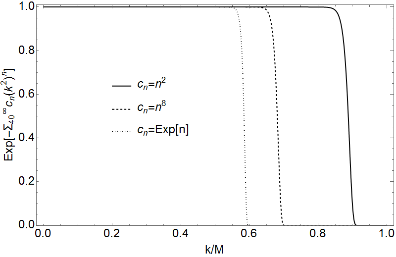
\displaystyle e^{-c_{n}\left(\frac{k^{2}}{M^{2}}\right)^{n}}\approx\left\{\begin{array}[]{lr}1,&\text{for }\frac{\sqrt[n]{c_{n}}k^{2}}{M^{2}}<1\\ 0,&\text{for }\frac{\sqrt[n]{c_{n}}k^{2}}{M^{2}}>1\end{array}\right\}.

Refer to caption — Figure 1: We plot $\exp\left[-\sum_{n=40}^{\infty}c_{n}\left(\frac{k^{2}}{M^{2}}\right)^{n}\right]$ for various $c_{n}$ to show that even if $c_{n}$ increases very quickly, we can model the higher terms in the polynomial $\gamma$ as the rectangle function Rect( $Ck^{2}/M^{2}$ ) without knowing the exact values of $c_{n}$ . Here $C$ is simply another constant to be found.

We can combine all of the terms in the exponential which involve large values of $n$ into a rectangle function and thus we do not need to know the value of $c_{n}$ for large $n$ as long as it is positive. As an example, we plot $\exp\left[-\sum_{n=40}^{\infty}c_{n}\left(\frac{k^{2}}{M^{2}}\right)^{n}\right]$ for various values of $c_{n}$ in Fig. 1 which turns out to still be well approximated by the rectangle function Rect( $Ck^{2}/M^{2}$ ) even if $c_{n}$ increases exponentially. In other words, the potential is well described by the lowest order terms and a single constant representing the higher order terms. ³³ 3 We need in the region of $\mathcal{O}(10)$ of the lower order terms depending on how accurate one needs to be.

III Perturbing the metric

Following the example of [62], we write the perturbation to the background de Sitter metric as

	$\displaystyle ds^{2}$	$\displaystyle=$	$\displaystyle-\left(1+2\Phi(r)-H^{2}r^{2}\right)dt^{2}$		(8)
			$\displaystyle+\left(1-2\Psi(r)\right)\left[\left(1+H^{2}r^{2}\right)dr^{2}+r^{2}d\Omega^{2}\right],$		(8)

where $\Phi(r)$ and $\Psi(r)$ are perturbations we want to find. As we want to look at perturbations at relatively short distances such as when we are looking at laboratory or solar system tests of gravity, we can use the approximation $H^{2}r^{2}\ll 1$ to find the Ricci curvature tensors and Ricci scalar up to linear order in $\Phi(r)$ and $\Psi(r)$

\displaystyle R_{tt}\approx\Delta\Phi(r)-3H^{2}\left(1+2\Psi(r)-\Phi(r)\right),

(9)

	$\displaystyle R_{rr}$	$\displaystyle\approx$	$\displaystyle\frac{2\left(r\Psi^{\prime\prime}(r)+\Psi^{\prime}(r)\right)}{r}-\Phi^{\prime\prime}(r)$		(10)
			$\displaystyle+H^{2}\bigg[3-r\Phi^{\prime}(r)-2\Phi(r)+4\Psi(r)\bigg],$		(10)

\displaystyle R\approx 4\Delta\Psi(r)-2\Delta\Phi(r)+12H^{2}\left(1+3\Psi(r)-\Phi(r)\right).~~~

(11)

We note that in the limit $H^{2}\hskip 0.85358ptr^{2}\ll 1$ , for any scalar $X(r)$ which is a function only of the radial coordinate [62],

\displaystyle\bar{\Box}X(r)\approx\Delta\ X(r),

(12)

where $\Delta$ $\equiv$ $\eta^{ij}\nabla_{i}\partial_{j}$ = $\partial_{r}^{2}\hskip-2.84526pt+\hskip-2.84526pt\frac{2}{r}\partial_{r}$ is the spatial d’Alembertian operator around a flat background. This gives us a tremendous simplification to our equations of motion, as we will see later.

IV Solving the equations of motion

We investigate a perturbation caused by the addition of a static point mass with density $\rho=m~\delta^{3}(\bf{x})$ where $m$ is the mass of the source and negligible pressure $P\approx 0$ . Using the equations of motion and $T^{\mu}_{\mu}=-\rho=T^{0}_{0}$ , we find $\Psi$ in terms of $\Phi$ in (18) and therefore find $\Phi$ in terms of our density $\rho$ in (19).

Using a similar method to [14] we can go into momentum space to find

\displaystyle\Phi(r)

\displaystyle=

\displaystyle\frac{m}{4\pi^{2}M^{2}_{P}\hskip 1.13809ptr}\int^{\infty}_{-\infty}dk~I(k).

(13)

where $I(k)$ , a complicated function of $H$ , $a(\Box)$ , $c(\Box)$ and $f(\Box)$ is given in (20).

For the value of $H$ at the current time $H$ = $H_{0}=7.25\times 10^{-27}$ m^-1, the result is very similar to the result around a flat background, and we plot this in Fig. 2. Perhaps this is to be expected - the differences from GR kick in only once we reach $k\approx M$ , and our mass scale is at a significantly higher energy than the Hubble parameter, i.e. for large $k$ , the background curvature has a negligible effect - for $H\ll k$ then the integrand is the same as for a flat background. We illustrate this by plotting in Fig. 3 and Fig. 4 the value of the integrand for small and large $k$ , choosing our value of $M$ to be the lower bound given by experiments [24].

Note that increasing $r$ decreases the value of $k$ in the region where it provides the biggest contribution to the integral.⁴⁴ 4 Due to the $\sin(kr)$ term, the part of the integrand where $k\ll r^{-1}$ can be neglected. Therefore for distances above the length scale where IDG contributes, around $10^{-5}$ m, we can use the GR prediction, and for distances at this length scale or below, we can use the IDG prediction around a flat background. Therefore we still obtain a non-singular potential even when we look at a curved background. At distances larger than the mass scale of IDG, the system returns to the standard de Sitter-Schwarzschild metric.

V Discussion

It was already shown that IDG gives a non-singular potential for a test mass added to a flat background, which returns to the GR prediction at large distances. Intuitively, one might have predicted this by noting that IDG has a significant effect at much larger energy scales than the curvature of our de Sitter universe. Here we have shown explicitly that in the region where the background curvature must be taken into account IDG has no effect, and where IDG has an effect the background curvature has no effect.

If we want to examine a system where $H$ is much larger than it is today, so that the background curvature can no longer be discarded, then it is possible to solve (13) numerically, as long as $H^{2}r^{2}\ll 1$ still holds.

Could our result be extended to more general backgrounds? It is extremely difficult to use the equations of IDG where we encounter derivatives in more than one coordinate, but it is reasonable to guess that if the background curvature is at an energy much smaller than the energy scale where IDG becomes important, then we will see a similar effect.

VI Conclusion

We have shown that the non-singular IDG potential that is found around a flat background also extends to a curved de Sitter background. It still reverts to the GR limit at large distances. We also show that only a finite number of the degrees of freedom in the theory actually contribute to the potential.

IDG is a promising model because it is ghost-free while allowing the possibility of avoiding singularities as well as providing a framework for inflation. This result shows that we can generate a non-singular potential even when we are looking at non-flat backgrounds, and hints that we will see similar effects when looking at more general backgrounds, based on examining the energy scales involved.

VII Acknowledgements

We would like to thank David Burton, Aindriú Conroy and David Sloan for their invaluable advice and suggestions in preparing this paper.

VIII Appendix

Appendix A Commutation relations

We want to write the linear equations of motion around a constantly curved background which is maximally symmetric, i.e. $\bar{R}^{\mu}{}_{\nu\rho\sigma}=\frac{\bar{R}}{12}\left(\delta^{\mu}_{\rho}g_{\nu\sigma}-\delta^{\mu}_{\sigma}g_{\nu\rho}\right)$ and $\bar{R}_{\mu\nu}=\frac{\bar{R}}{4}g_{\mu\nu}$ .

We use the relations from the appendix of [39] and also derive that for a scalar $S$ ,

	$\displaystyle\nabla^{\mu}F(\Box)\nabla_{\nu}S=F(\Box-5H^{2})\nabla^{\mu}\nabla_{\nu}S$
	$\displaystyle+\frac{1}{4}\left(F(\Box+3H^{2})-F(\Box-5H^{2})\right)\delta^{\mu}_{\nu}\Box S,$		(14)

and that for a symmetric tensor $t_{\mu\nu}$

\displaystyle\nabla_{\mu}F(\Box)t^{\mu\nu}=F\left(\Box+5H^{2}\right)\nabla_{\mu}t^{\mu\nu}-2H^{2}X(\Box)\nabla_{\nu}t^{\mu}_{\mu},~~~~~~

(15)

where we have defined

\displaystyle X(\Box)\equiv\sum^{\infty}_{n=1}f_{n}\sum_{m=0}^{n-1}\left[\left(\Box+5H^{2}\right)^{m}\left(\Box-3H^{2}\right)^{n-1-m}\right].~~~~~~~

(16)

Appendix B Full equations of motion

Using the commutation relations above, we can write the equations of motion as (2) with

	$\displaystyle a(\Box)\equiv 1+24M^{-2}_{p}H^{2}\tilde{f}_{1_{0}}+(\Box-2H^{2})M^{-2}_{p}F_{2}(\Box),$
	$\displaystyle c(\Box)\equiv 1+M^{-2}_{p}\Big\{24H^{2}\tilde{f}_{1_{0}}-4(\Box+3H^{2})F_{1}(\Box)$
	$\displaystyle-\frac{1}{2}F_{2}(\Box+8H^{2})\Box-\frac{1}{2}F_{2}(\Box)(\Box+8H^{2})+4H^{2}\Box F_{2}^{\prime}(\Box)\Big\},$
	$\displaystyle f(\Box)\equiv M^{-2}_{p}\left(4F_{1}(\Box)+2F_{2}(\Box)-8H^{2}X(\Box-5H^{2})\right),~~~~~~$		(17)

and we can therefore find $\Psi$ in terms of $\Phi$

\displaystyle\hskip-6.54413pt\frac{\Psi(r)}{\Phi(r)}\hskip-1.99168pt=\hskip-1.99168pt\frac{a(\Delta)(\Delta+3H^{2})-\left(3c(\Delta)+\Delta f(\Delta)\right)\left(\Delta+6H^{2}\right)}{a(\Delta)(4\Delta+30H^{2})-2\left(3c(\Delta)+\Delta f(\Delta)\right)\left(\Delta+9H^{2}\right)},~~~~~~

(18)

and therefore find $\Phi$ in terms of our density $\rho$

\displaystyle\hskip-13.94182pt\Phi(r)\hskip-2.84526pt=\hskip-2.84526pt\frac{\rho\left(a(\Delta)(2\Delta+15H^{2})-\left(3c(\Delta)+\Delta f(\Delta)\right)\left(\Delta+9H^{2}\right)\right)}{M^{2}_{P}a(\Delta)\left[2a(\Delta)-4c(\Delta)-\Delta f(\Delta)\right]\left(\Delta^{2}+15H^{2}\Delta+63H^{4}\right)}.\hskip 1.13809pt~~~~~

(19)

By going into momentum space, i.e. sending $\Delta\to-k^{2}$ , taking a Fourier transform and using $\rho=m\hskip 2.27621pt\delta^{3}(\textbf{x})$ , we can write $\Phi(r)$ as an integral we can solve

\displaystyle\Phi(r)

\displaystyle=

\displaystyle\frac{m}{4\pi^{2}M^{2}_{P}r}\int^{\infty}_{-\infty}dk~k\sin(kr)\frac{a(-k^{2})(-4k^{2}+30H^{2})-2\left(3c(-k^{2})-k^{2}f(-k^{2})\right)\left(-k^{2}-18H^{2}\right)}{a(-k^{2})\left(2a(-k^{2})-4c(-k^{2})+k^{2}f(-k^{2})\right)\left(k^{4}-15H^{2}k^{2}+63H^{4}\right)}.

(20)

which is written in the main text as (13).

References

[1] C. M. Will, Living Rev. Relativity, 17, (2014), 4 “The Confrontation between General Relativity and Experiment,” doi:10.12942/lrr-2014-4
[2] B. P. Abbott et al. [LIGO Scientific and Virgo Collaborations], “GW170817: Observation of Gravitational Waves from a Binary Neutron Star Inspiral,” Phys. Rev. Lett. 119 (2017) no.16, 161101 doi:10.1103/PhysRevLett.119.161101 [arXiv:1710.05832 [gr-qc]].
[3] S. W. Hawking and G. F. R. Ellis, “The Large Scale Structure of Space-Time,” doi:10.1017/CBO9780511524646
[4] A. Raychaudhuri, “Relativistic cosmology. 1.,” Phys. Rev. 98 (1955) 1123. doi:10.1103/PhysRev.98.1123
[5] K. S. Stelle, “Renormalization of Higher Derivative Quantum Gravity,” Phys. Rev. D 16 (1977) 953. doi:10.1103/PhysRevD.16.953
[6] L. Modesto, T. de Paula Netto and I. L. Shapiro, “On Newtonian singularities in higher derivative gravity models,” JHEP 1504 (2015) 098 doi:10.1007/JHEP04(2015)098 [arXiv:1412.0740 [hep-th]].
[7] B. L. Giacchini, “On the cancellation of Newtonian singularities in higher-derivative gravity,” Phys. Lett. B 766 (2017) 306 doi:10.1016/j.physletb.2017.01.019 [arXiv:1609.05432 [hep-th]].
[8] N. Barnaby and N. Kamran, “Dynamics with infinitely many derivatives: The Initial value problem,” JHEP 0802 (2008) 008 doi:10.1088/1126-6708/2008/02/008 [arXiv:0709.3968 [hep-th]].
[9] P. Van Nieuwenhuizen, “On ghost-free tensor lagrangians and linearized gravitation,” Nucl. Phys. B 60 (1973) 478. doi:10.1016/0550-3213(73)90194-6
[10] R. P. Woodard, “Ostrogradsky’s theorem on Hamiltonian instability,” Scholarpedia 10 (2015) no.8, 32243 doi:10.4249/scholarpedia.32243 [arXiv:1506.02210 [hep-th]].
[11] M. Ostrogradsky, “Mémoires sur les équations différentielles, relatives au problème des isopérimètres,” Mem. Acad. St. Petersbourg 6 (1850) no.4, 385.
[12] A. A. Tseytlin, “On singularities of spherically symmetric backgrounds in string theory,” Phys. Lett. B 363 (1995) 223 doi:10.1016/0370-2693(95)01228-7 [hep-th/9509050].
[13] T. Biswas, A. and W. Siegel, “Bouncing universes in string-inspired gravity,” JCAP 0603 (2006) 009 doi:10.1088/1475-7516/2006/03/009 [hep-th/0508194].
[14] T. Biswas, E. Gerwick, T. Koivisto and A. , “Towards singularity and ghost free theories of gravity,” Phys. Rev. Lett. 108 (2012) 031101 doi:10.1103/PhysRevLett.108.031101 [arXiv:1110.5249 [gr-qc]].
[15] T. Biswas, A. S. Koshelev and A. Mazumdar, “Gravitational theories with stable (anti-)de Sitter backgrounds,” Fundam. Theor. Phys. 183 (2016) 97 doi:10.1007/978-3-319-31299-6 [arXiv:1602.08475 [hep-th]].
[16] E. Tomboulis, “Renormalizability and Asymptotic Freedom in Quantum Gravity,” Phys. Lett. B 97, 77 (1980).
[17] W. Siegel, “Stringy gravity at short distances,” hep-th/0309093.
[18] T. Biswas, T. Koivisto and A. Mazumdar, “Nonlocal theories of gravity: the flat space propagator,” arXiv:1302.0532 [gr-qc].
[19] L. Buoninfante, “Ghost and singularity free theories of gravity,” arXiv:1610.08744 [gr-qc].
[20] S. Talaganis, T. Biswas and A. Mazumdar, “Towards understanding the ultraviolet behavior of quantum loops in infinite-derivative Class. Quant. Grav. 32 (2015) no.21, 215017 doi:10.1088/0264-9381/32/21/215017 [arXiv:1412.3467 [hep-th]].
[21] A. S. Koshelev, K. S. Kumar and P. V. Moniz, “Effective models of inflation from a nonlocal framework,” Phys. Rev. D 96 (2017) no.10, 103503 doi:10.1103/PhysRevD.96.103503 [arXiv:1604.01440 [hep-th]].
[22] A. S. Koshelev, K. Sravan Kumar and A. A. Starobinsky, “ $R^{2}$ inflation to probe non-perturbative quantum gravity,” arXiv:1711.08864 [hep-th].
[23] L. Modesto, “Super-renormalizable Quantum Gravity,” Phys. Rev. D 86 (2012) 044005 doi:10.1103/PhysRevD.86.044005 [arXiv:1107.2403 [hep-th]]; “Super-renormalizable Multidimensional Quantum Gravity,” Astron. Rev. 8.2 (2013) 4-33 [arXiv:1202.3151 [hep-th]]; L. Modesto and L. Rachwal, “Super-renormalizable and finite gravitational theories,” Nucl. Phys. B 889 (2014) 228 doi:10.1016/j.nuclphysb.2014.10.015 [arXiv:1407.8036 [hep-th]]; “Finite Conformal Quantum Gravity and Nonsingular Spacetimes,” arXiv:1605.04173 [hep-th]
[24] J. Edholm, A. S. Koshelev and A. Mazumdar, “Universality of testing ghost-free gravity,” arXiv:1604.01989 [gr-qc]. Phys. Rev. D 94 (2016) no.10, 104033 doi:10.1103/PhysRevD.94.104033
[25] A. Conroy, T. Koivisto, A. Mazumdar and A. Teimouri, “Generalized quadratic curvature, non-local infrared modifications of gravity and Newtonian potentials,” Class. Quant. Grav. 32 (2015) no.1, 015024 doi:10.1088/0264-9381/32/1/015024 [arXiv:1406.4998 [hep-th]].
[26] J. Edholm and A. Conroy, “Newtonian Potential and Geodesic Completeness in Infinite Derivative Gravity,” Phys. Rev. D 96 (2017) no.4, 044012 doi:10.1103/PhysRevD.96.044012 arXiv:1705.02382 [gr-qc].
[27] A. S. Cornell, G. Harmsen, G. Lambiase and A. Mazumdar, “Rotating metric in Non-Singular Infinite Derivative Theories of Gravity,” arXiv:1710.02162 [gr-qc].
[28] J. Edholm and A. Conroy, “Criteria for resolving the cosmological singularity in Infinite Derivative Gravity around expanding backgrounds,” arXiv:1710.01366 [gr-qc]. Phys. Rev. D 96 (2017) 124040 doi:10.1103/PhysRevD.96.124040
[29] Y. S. Myung and Y. J. Park, “The origin of regular Newtonian potential in infinite derivative gravity,” arXiv:1709.04587 [gr-qc].
[30] V. P. Frolov and A. Zelnikov, “Head-on collision of ultra-relativistic particles in ghost-free theories of gravity,” arXiv:1509.03336 [hep-th].
[31] V. P. Frolov, “Mass-gap for black hole formation in higher derivative and ghost free gravity,” Phys. Rev. Lett. 115, no. 5, 051102 (2015) [arXiv:1505.00492 [hep-th]].
[32] V. P. Frolov, A. Zelnikov and T. de Paula Netto, “Spherical collapse of small masses in the ghost-free gravity,” JHEP 1506, 107 (2015) [arXiv:1504.00412 [hep-th]].
[33] T. Biswas, A. Conroy, A. S. Koshelev and A. Mazumdar, “Generalized ghost-free quadratic curvature gravity,” Class. Quant. Grav. 31 (2014) 015022 Erratum: [Class. Quant. Grav. 31 (2014) 159501] doi:10.1088/0264-9381/31/1/015022, 10.1088/0264-9381/31/15/159501 [arXiv:1308.2319 [hep-th]].
[34] G. Calcagni, L. Modesto and P. Nicolini, “Super-accelerating bouncing cosmology in asymptotically-free non-local gravity,” Eur. Phys. J. C 74 (2014) no.8, 2999 doi:10.1140/epjc/s10052-014-2999-8 [arXiv:1306.5332 [gr-qc]].
[35] T. Biswas, A. S. Koshelev, A. Mazumdar and S. Y. Vernov, “Stable bounce and inflation in non-local higher derivative cosmology,” JCAP 1208 (2012) 024 doi:10.1088/1475-7516/2012/08/024 [arXiv:1206.6374 [astro-ph.CO]].
[36] T. Biswas, T. Koivisto and A. Mazumdar, “Towards a resolution of the cosmological singularity in non-local higher derivative theories of gravity,” JCAP 1011 (2010) 008 doi:10.1088/1475-7516/2010/11/008 [arXiv:1005.0590 [hep-th]].
[37] A. S. Koshelev and S. Y. Vernov, “On bouncing solutions in non-local gravity,” Phys. Part. Nucl. 43 (2012) 666 doi:10.1134/S106377961205019X [arXiv:1202.1289 [hep-th]].
[38] A. S. Koshelev, “Stable analytic bounce in non-local Einstein-Gauss-Bonnet cosmology,” Class. Quant. Grav. 30 (2013) 155001 doi:10.1088/0264-9381/30/15/155001 [arXiv:1302.2140 [astro-ph.CO]].
[39] T. Biswas, A. S. Koshelev and A. Mazumdar, “Consistent Higher Derivative Gravitational theories with stable de Sitter and Anti-de Sitter Backgrounds,” arXiv:1606.01250 [gr-qc].
[40] A. Conroy, A. Mazumdar, S. Talaganis and A. Teimouri, “Nonlocal gravity in D dimensions: Propagators, entropy, and a bouncing cosmology,” Phys. Rev. D 92, no. 12, 124051 (2015) doi:10.1103/PhysRevD.92.124051 [arXiv:1509.01247 [hep-th]].
[41] A. Teimouri, S. Talaganis, J. Edholm and A. Mazumdar, “Generalised Boundary for Higher Derivative Theories of Gravity,” arXiv:1606.01911 [gr-qc]. JHEP 1608 (2016) 144 doi:10.1007/JHEP08(2016)144
[42] S. Talaganis and A. Teimouri, “Hamiltonian Analysis for Infinite Derivative Field Theories and Gravity,” arXiv:1701.01009 [hep-th].
[43] L. Modesto, J. W. Moffat and P. Nicolini, “Black holes in an ultraviolet complete quantum gravity,” Phys. Lett. B 695 (2011) 397 doi:10.1016/j.physletb.2010.11.046 [arXiv:1010.0680 [gr-qc]].
[44] V. P. Frolov and A. Zelnikov, “Radiation from an emitter in the ghost free scalar theory,” Phys. Rev. D 93 (2016) no.10, 105048 doi:10.1103/PhysRevD.93.105048 [arXiv:1603.00826 [hep-th]].
[45] G. Calcagni and L. Modesto, “Nonlocal quantum gravity and M-theory,” Phys. Rev. D 91 (2015) no.12, 124059 doi:10.1103/PhysRevD.91.124059 [arXiv:1404.2137 [hep-th]].
[46] L. Feng, “Light Bending in the Infinite Derivative Theories of Gravity,” Phys. Rev. D 95 (2017) no.8, 084015 doi:10.1103/PhysRevD.95.084015 arXiv:1703.06535 [gr-qc].
[47] G. Calcagni and G. Nardelli, “Non-local gravity and the diffusion equation,” Phys. Rev. D 82 (2010) 123518 doi:10.1103/PhysRevD.82.123518 [arXiv:1004.5144 [hep-th]].
[48] A. S. Koshelev and A. Mazumdar, “Do massive compact objects without event horizon exist in infinite derivative gravity?,” Phys. Rev. D 96 (2017) no.8, 084069 doi:10.1103/PhysRevD.96.084069 arXiv:1707.00273 [gr-qc].
[49] A. Ghoshal, A. Mazumdar, N. Okada and D. Villalba, “On the Stability of Infinite Derivative Abelian Higgs,” arXiv:1709.09222 [hep-th].
[50] G. Calcagni and L. Modesto, “Stability of Schwarzschild singularity in non-local gravity,” Phys. Lett. B 773 (2017) 596 doi:10.1016/j.physletb.2017.09.018 [arXiv:1707.01119 [gr-qc]]
[51] N. Arkani-Hamed, S. Dimopoulos, G. Dvali and G. Gabadadze, “Nonlocal modification of gravity and the cosmological constant problem,” hep-th/0209227.
[52] J. Edholm, “UV completion of the Starobinsky model, tensor-to-scalar ratio, and constraints on nonlocality,” Phys. Rev. D 95 (2017) no.4, 044004 doi:10.1103/PhysRevD.95.044004 [arXiv:1611.05062 [gr-qc]].
[53] F. Briscese, A. Marcianò, L. Modesto and E. N. Saridakis, “Inflation in (Super-)renormalizable Gravity,” Phys. Rev. D 87 (2013) no.8, 083507 doi:10.1103/PhysRevD.87.083507 [arXiv:1212.3611 [hep-th]].
[54] A. S. Koshelev, L. Modesto, L. Rachwal and A. A. Starobinsky, “Occurrence of exact $R^{2}$ inflation in non-local UV-complete gravity,” JHEP 1611 (2016) 067 doi:10.1007/JHEP11(2016)067 [arXiv:1604.03127 [hep-th]].
[55] B. Craps, T. De Jonckheere and A. S. Koshelev, “Cosmological perturbations in non-local higher-derivative gravity,” JCAP 1411 (2014) no.11, 022 doi:10.1088/1475-7516/2014/11/022 [arXiv:1407.4982 [hep-th]].
[56] S. Talaganis, “Quantum Loops in Non-Local Gravity,” PoS CORFU 2014 (2015) 162 [arXiv:1508.07410 [hep-th]].
[57] S. Talaganis, “Towards UV Finiteness of Infinite Derivative Theories of Gravity and Field Theories,” arXiv:1704.08674 [hep-th].
[58] A. Conroy, A. S. Koshelev and A. Mazumdar, “Criteria for resolving the cosmological singularity in Infinite Derivative Gravity,” arXiv:1605.02080 [gr-qc].
[59] A. Conroy, “Infinite Derivative Gravity: A Ghost and Singularity-free Theory,” arXiv:1704.07211 [gr-qc].
[60] A. Conroy, A. S. Koshelev and A. Mazumdar, “Geodesic completeness and homogeneity condition for cosmic inflation,” Phys. Rev. D 90 (2014) no.12, 123525 doi:10.1103/PhysRevD.90.123525 [arXiv:1408.6205 [gr-qc]].
[61] L. Buoninfante, A. S. Koshelev, G. Lambiase and A. Mazumdar, “Classical properties of non-local, ghost- and singularity-free gravity,” arXiv:1802.00399 [gr-qc].
[62] X. H. Jin, D. J. Liu and X. Z. Li, “Solar System tests disfavor f(R) gravities,” astro-ph/0610854.
[63] S. B. Lambert and C. Le Poncin-Lafitte, “Determination of the relativistic parameter gamma using very long baseline interferometry,” Astron. Astrophys. 499 (2009) 331 doi:10.1051/0004-6361/200911714 [arXiv:0903.1615 [gr-qc]].
[64] D. J. Kapner, T. S. Cook, E. G. Adelberger, J. H. Gundlach, B. R. Heckel, C. D. Hoyle and H. E. Swanson, “Tests of the gravitational inverse-square law below the dark-energy length scale,” Phys. Rev. Lett. 98 (2007) 021101
[65] L. Perivolaropoulos, “Sub-millimeter Spatial Oscillations of Newton’s Constant: Theoretical arXiv:1611.07293 [gr-qc].

Revealing Infinite Derivative Gravity’s true potential: The weak-field limit around de Sitter backgrounds