Probing the electroweak phase transition
via enhanced di-Higgs boson production
Abstract
We consider a singlet extension of the Standard Model (SM) with a spontaneous breaking and study the gluon-gluon fusion production of the heavy scalar, with subsequent decay into a pair of SM-like Higgs bosons. We find that an on-shell interference effect can notably enhance the resonant di-Higgs production rate up to 40%. In addition, consistently taking into account both the on-shell and off-shell interference effects between the heavy scalar and the SM di-Higgs diagrams significantly improves the HL-LHC and HE-LHC reach in this channel. As an example, within an effective field theory analysis in an explicitly breaking scenario, we further discuss the potential to probe the parameter region compatible with a first order electroweak phase transition. Our analysis is applicable for general potentials of the singlet extension of the SM as well as for more general resonance searches.
Keywords
Higgs, Higgs pair, LHC, Phase Transition, HE-LHC, HL-LHC1 INTRODUCTION
Probing the intriguing possibility of electroweak baryogenesis [1, 2, 3, 4, 5] becomes of higher relevance after the SM Higgs boson discovery at the LHC [6, 7]. In such mechanism, a strongly first-order electroweak phase transition (EWPT) is a crucial ingredient to maintain the matter-antimatter asymmetry generated at the electroweak scale [8]. The SM Higgs potential is insufficient to provide such condition and many extensions of the SM have hence been proposed [9, 10, 11, 12, 13, 14, 15, 16, 17, 18, 19, 20, 21, 22, 23, 24, 25, 26, 27, 28, 29, 30, 31, 32, 33, 34, 35, 36, 37, 38, 39, 40, 41, 42]. Generically, including additional bosonic degrees of freedom with sizable coupling strength to the SM Higgs boson can increase the barrier between the broken and unbroken electroweak vacua at the critical temperature of the phase transition, see e.g., Ref. [43]. Amongst many of the possibilities, the singlet scalar extension of the SM is of particular interest [26, 27, 28, 29]. Due to its singlet nature, the scalar is hard to be probed at the LHC. Therefore the singlet SM extension serves as the simplest, yet elusive benchmark to test a sufficiently strong first-order phase transition compatible with the Higgs boson mass measurements at the LHC [26, 25].
The scalar potential of a real singlet scalar extension of the SM can be further categorized into three types, depending on the behavior of the real singlet under the parity operation , namely: the symmetric, the spontaneous breaking, and the general potential. The symmetric potential leads to a stable singlet scalar, resulting in the singlet being a possible dark matter candidate and yielding missing energy signals at colliders [26]. Without protection, the singlet would mix with the SM Higgs and (in most cases) a promptly decaying scalar particle would provide a rich phenomenology at colliders. The singlet scalar could be produced resonantly and decay back to pairs of SM particles, dominantly into , , and . The signal of a singlet scalar resonance decaying into is a smoking-gun for singlet enhanced EWPT [44, 45, 29, 28, 46, 47, 48, 49, 50].
Searches for resonant di-Higgs production have received much attention by both the ATLAS and CMS collaborations [51, 52, 53, 54, 55, 56]. In the case of a singlet resonance, constraints from SM precision measurements render these searches more challenging. From one side precision measurements imply that the singlet-doublet mixing parameter is constrained to be small over a large region of parameter space. From the other side, the singlet only couples to SM particles through mixing with the SM Higgs doublet. This results in a reduced di-Higgs production via singlet resonance decays. In particular, the singlet resonance amplitude becomes of the same order as the SM triangle and box diagram amplitudes. Most important, in this work we shall show that a large relative phase between the SM box diagram and the singlet triangle diagram becomes important. This special on-shell interference effect has been commonly overlooked in the literature and turns out to have important phenomenological implications. We shall choose the spontaneous breaking scenario of the SM plus singlet to demonstrate the importance of the novel on-shell interference effect for the resonant singlet scalar searches in the di-Higgs production mode.
Our paper is organized as follows. In Sec. 2, we study the details of the symmetric potential with spontaneous and electroweak symmetry breaking, including its parametric dependence on physical quantities, requirements of vacuum stability and perturbative unitarity, and the decay properties of the singlet scalar. In Sec. 3, we present a detailed discussion on various types of interference effects for the process . We focus on the special case of the on-shell interference effect for the resonant singlet production and show their parametric dependence. In Sec. 4, we study the impact of the on-shell interference effect for the High Luminosity (HL)- and High Energy (HE)- LHC searches and address how a comprehensive study of the on-shell and off-shell differential cross sections would improve on their sensitivity. This in turn will provide the tools for a much more robust test of a strongly first-order EWPT in this type of models. We reserve Sec. 5 for our conclusions.
2 MODEL FRAMEWORK
We will consider the simplest extension of the SM that can assist the scalar potential to induce a strongly first-order electroweak phase transition, consisting of an additional real scalar singlet with a symmetry. The scalar potential of the model can be written as
| (1) |
where is the SM doublet 11 1 , where are the Goldstone modes. and represents the new real singlet field. In the above, we adopt the conventional normalization for the couplings of the SM doublets and match the other couplings with the singlet with identical normalization. We allow for spontaneous breaking with the singlet acquiring a vacuum expectation value (vev) , since this case allows for interesting collider phenomenology of interference effects. As we shall show later, the (on-shell) interference effects commonly exist for loop-induced processes in BSM phenomenology and it is the focus of this paper. The CP even neutral component of the Higgs doublet field mixes with the real singlet scalar , defining the new mass eigenstates and
| (2) |
where is the mixing angle between these fields. The five free parameters in Eq. (1) can be traded by the two boundary conditions
| (3) |
and the three “physical” parameters,
| (4) |
where characterizes the ratio between the vevs of the doublet and the singlet scalar fields, respectively.
As a result, the parameters in the scalar potential in Eq. (1) can be expressed as functions of these new parameters,
| (5) | |||||
| (6) | |||||
| (7) | |||||
| (8) | |||||
| (9) |
Observe that the condition of spontaneous symmetry breaking implies that dimensionful quantities and can be directly expressed in terms of the original quartic couplings and the vevs,
| (10) |
2.1 Stability, unitarity and EWSB conditions


It is useful to understand the quartic couplings in the potential in Eq. (1) in terms of the physical parameters defined in Eq. (4), since the physical parameters make a straightforward connection with collider physics. In Fig. 1 we show the three independent quartic couplings in the -symmetric potential , and in blue, red, and black contours, respectively, as a function of the heavy singlet-like scalar mass and the singlet-doublet mixing angle for = 1 (left panel) and = 10 (right panel). As shown in the red contours, for low values of , a large quartic is needed to obtain a heavy singlet, due to the fact that the singlet mass and its vev are related via its quartic coupling, see Eq. (8). However, the correlation between the singlet quartic, its mass and its vev is only mildly dependent on the mixing angle . A different behavior occurs for the Higgs quartic, in blue, being independent of the singlet vev but sensitive to the mixing angle.
The stability of the potential and the perturbative unitarity arguments set constraints on the allowed sizes and signs of the quartic couplings that we will discuss now. The requirement of the potential being bounded from below leads to the conditions to the quartic couplings
| (11) |
The positivity of the Higgs and singlet quartic couplings is understood by considering large field values in the directions and . The extra condition arises from considering large field values in an arbitrary direction. We see that negative values for the mixing quartic coupling are allowed if the other two quartics are large enough.
Furthermore, the spontaneous and electroweak symmetry breaking vacuum is a global minimum if the following is satisfied
| (12) |
For larger values of , the electroweak and breaking vacuum becomes a saddle point and the minima are located at and 22 2 Note that the expressions for the vevs in terms of model parameters differ for the different extrema under discussion. We denote them using the same symbols, and , since the discussion in this section does not rely on their precise values.. Observe that for positive values of and the origin is always a maximum.
The conditions Eq. (11) and Eq. (12) have the following physical interpretation. The determinant of the mass matrix at the electroweak and breaking minimum is proportional to , which is equivalent to the previous requirements. When the determinant of the mass matrix becomes negative, and therefore one of the conditions fails, a tachyonic direction will be generated, destabilizing the system and evolving it to other minima. From this perspective it is also clear that if we choose to work with as a set of parameters, the determinant of the mass matrix is just and the requirements in this basis are automatically satisfied with physical masses.
The potential might be destabilized due to loop corrections, and the quantity might become negative at high scales. We study this effect taking into account the renormalization group evolution (RGE) of the quartic couplings given by the RGE equations in Sec. A. In Fig. 2 we show, shaded in red, the region where the vacuum becomes unstable at a given energy scale. For small singlet masses and mixing angles the instability scale is not modified with respect to the SM (which is around GeV at one loop and relaxes to about GeV once two-loop RGE is included [57]), but for larger mixings the singlet shifts the values of the couplings, pushing the scale of instability to larger values. For larger , as shown in the right panel of Fig. 2, the singlet quartic coupling are smaller and the instability condition extends to a larger region since the effect of the singlet is insufficient to compensate the effect of the destabilizing top Yukawa coupling.
There is also a constraint on the size of the quartic couplings given by the perturbative unitarity arguments. The amplitudes should satisfy
| (13) |
This comes from decomposing the amplitude in partial waves and requiring it being consistent with the optical theorem. We consider the different scattering amplitudes among the components of the Higgs doublet and the singlet, and look for the combination of states giving the largest contribution to Eq. (13). This is done by building a matrix that contains all the amplitudes among those states and taking the largest eigenvalue. We derive the constraints on the sizes of the quartic couplings by this method, giving further details in Sec. A.
In Fig. 2, the gray shaded regions show the constraints from the perturbative unitarity arguments after including the RGE effects, labeled by the scale at which unitarity is broken. We observe that smaller values of and larger singlet masses have a lower unitarity breaking scale. This is due to the fact that larger singlet masses require larger singlet quartic couplings. In addition, larger corresponds to larger vevs of the singlet and yields larger masses for smaller values of the quartic couplings. Hence perturbative unitarity arguments are relaxed as increases as well as for smaller values of .
2.2 Properties of the singlet-like scalar
In addition to the effect of singlet-doublet mixing governed by , the relevant phenomenology of the production of di-Higgs final states is further characterized by two trilinear coupling parameters
| (14) |
The dimensionful parameter is the modified trilinear Higgs coupling and is the heavy Scalar-Higgs-Higgs coupling that drives the heavy scalar decay into the di-Higgs final state. Both couplings can be written in terms of the physical parameters , and as
| (15) | |||||
| (16) |
In Fig. 3, we show the values of trilinear couplings between mass eigenstates, and in green and magenta curves, as a function of the heavy singlet-like scalar mass and the singlet-doublet mixing angle for = 1 (left panel) and = 10 (right panel). We can observe that the trilinear coupling of the SM-like Higgs remains insensitive to the singlet mass and receives moderate modifications with respect to its SM value. On the other hand, the trilinear that determines the rate of the heavy scalar decay into Higgs pairs is quite sensitive to the precise value of the singlet-like scalar mass and the mixing angle .
The heavy singlet mixing with the SM Higgs will induce a global shift on all the SM-like Higgs couplings. While this mixing does not change the SM branching ratios, the production rates of the Higgs boson will be reduced by a factor . The Higgs boson data from LHC at 7 and 8 TeV sets a constraint of at 95% C.L., independently of the singlet mass. The HL-LHC projection increases this limit very mildly due to the dominant effect from systematic and theory uncertainties. In addition, the current limit is driven by a measured - excess of signal strength over the SM Higgs expectation. Moreover, the singlet mixing affects the electroweak precision observables (EWPO) measured at LEP, setting slightly stronger limits than those coming from Higgs physics. Hence, in Fig. 3 we only show as brown shaded regions those excluded by EWPO, and refer to Sec. B for a detailed discussion. We also show in gray the region disallowed by vacuum stability and perturbative unitarity arguments at the scale where the physical parameters are defined, as discussed in the previous section.
Let’s now discuss the decay properties of the singlet like scalar. Its decay to Higgs pairs is governed by the trilinear coupling
| (17) |
and to other SM particles via its mixing with the SM Higgs. The total singlet like scalar width can be written as,
| (18) |
where is the total width of a SM Higgs with mass .
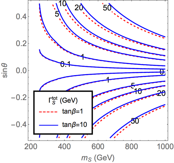

In the left panel of Fig. fig:scalardecay, we show the total width of the heavy scalar state as a function of its mass and the mixing angle for values of 1 and 10. We can see that its total width is not particularly sensitive to . On the right panel of Fig. 4, we show the singlet decay branching ratio to Higgs pairs in the plane of the singlet scalar mass and the singlet-doublet mixing angle for of 1 (red, dashed lines) and 10 (blue, solid lines), respectively. The branching fraction features a rapid decrease of roughly 5% near the threshold due to the opening of this new decay channel. In addition, due to the possible cancellation from contributions to the trilinear coupling in parameter space, as depicted in Eq. (16), one can see strong variations in contour shapes for each value of .
The partial width of the singlet to Higgs bosons scales as the third power of the scalar mass for a heavy scalar. This can be easily understood from Eq. (16) and Eq. (17). The partial width to and through the mixing with the SM Higgs also grows as the third power of the scalar mass due to the longitudinal enhancement for the massive vector gauge bosons. Consequently, the singlet branching fraction to remains in the 20% to 40% range over a large span of the parameter space.
3 ENHANCING THE DI-HIGGS SIGNAL VIA INTERFERENCE EFFECTS
The on-shell interference effect may enhance or suppress the conventional Breit-Wigner resonance production. Examples in Higgs physics known in the literature, such as [58] and [59], are both destructive. We discuss in detail in this section the on-shell interference effect between the resonant singlet amplitude and the SM di-Higgs box diagram. We shall show that in the singlet extension of the SM considered in this paper, the on-shell interference effect is generically constructive and could be large in magnitude, thus enhances the signal production rate.
3.1 Anatomy of the interference effect
The interference effect between two generic amplitudes can be denoted as nonresonant amplitude and resonant amplitude . The resonant amplitude , defined as
| (19) |
has a pole in the region of interest and we parametrize it as the product of a fast varying piece containing its propagator and a slowly varying piece that generically is a product of couplings and loop-functions. The general interference effect can then be parameterized as [59, 58],
| (20) |
where and denote the complex phases of and , respectively.
Schematically, the three amplitudes that enter the di-Higgs production can be parametrized as the following,
| (21) | |||||
| (22) | |||||
| (23) |
where and are the corresponding loop functions. In Eq. (21) we have dropped the nonimportant factors for the SM Higgs total width as the pair production is far above the SM Higgs on-shell condition. For a CP-conserving theory that we are considering, all of the above parameters are real, except for the loop-functions and . The relevant phase between these loop functions33 3 These loop functions can also be understood as form factors of the effective gluon-gluon-Higgs(-Higgs) couplings. induces nontrivial interference effect between these diagrams.
The detailed expressions for these three amplitudes can be found in Ref. [60]. The SM box contribution contains two pieces and . The piece corresponds to different helicity combinations of the gluons that does not interfere with the resonant term. In Fig. 5, we show as a function of the partonic center of mass energy , the phases of the triangle and box loop functions and their relative phase in blue, magenta and yellow curves, respectively. We observe that the phases of both diagrams start to increase after the threshold, as expected from the optical theorem. In particular, the relative phase between the interfering box and triangle diagrams, shown as the yellow curves, grows quickly after the threshold and remains large for the entire region under consideration. This relative strong phase drives the physics discussed in this paper as it allows for a nonvanishing interference effect between the singlet resonance diagram and the SM box diagram.
| Inter. Term. | Rel. phase | Proportionality | Inter. sign | |
|---|---|---|---|---|
| - | ||||
| 0 | ||||
| - | 1 | |||
| 0 | 0 | |||
| - | ||||
In Table 1, we summarize the different behaviors of all the interference terms allowed in this theory. We decompose the interference effects into the and , as defined in Eq. (20), and further highlight their dependence on the relative phase, model parameters and the resulting signs of the interference effects.
The special terms vanish both for the interference between the SM diagrams - and the interference between the resonant singlet and the SM triangle diagrams - for different reasons. For the latter, the singlet resonant amplitude and the SM triangle amplitude share a common source of the strong phase from the triangle fermionic loop of the induced gluon-gluon-scalar coupling. Hence, and this makes Eq. (20) vanish. For the interference between the SM box and triangle diagrams -, denoted in the proportionality column of the table, the vanishes because we are always in the off-shell regime for the intermediate SM Higgs in the triangle diagram. Viewing the SM triangle diagram as , then the part in Eq. (20) is strictly nonzero. However, due to the fact that we can never hit the SM Higgs pole in the relevant regime , such contribution is
| (24) |
and hence can be neglected.
In contrast, the special interference effect only appears between the singlet resonant diagram and the SM box digram -. This interference effect is proportional to the relative phase between the loop functions and the imaginary part of the scalar propagator which is sizable near the scalar mass pole. In this work, we pay special attention to this effect whose importance has been overlooked in the past literature.
The signs of the interference effects are determined by a product of relative phases, model parameters and kinematics. The relative phases are always positive for the mass range considered here, as shown in Fig. 5. The kinematics straightforwardly relies on the Higgs pair invariant mass with respect to the heavy scalar mass pole. In addition due to spontaneously breaking model construction and consistency requirement, and has opposite signs, in accordance to the sign of in the original potential. The overall signs of the interference effects end up being fixed as shown in Table 1.
3.2 Parametric dependence of the on-shell interference effect
After understanding the sources of various interference effects, especially the on-shell interference effect , we study its parametric dependence in this section.44 4 Throughout this work we use the finite result at leading order [60]. We adopt the K-factor between the next-to-leading-order and the leading-order result in the distribution provided by Ref. [45].
We first show the line-shape decomposition into components discussed in Table 1 for two benchmark points in Fig. 6. We display the Breit-Wigner, nonresonant line shape from SM triangle and box diagrams, and the total line shape in red, brown and black curves, respectively. The interference terms proportional to the real part of the heavy scalar propagator are shown in blue and magenta curves. Observe that these interference terms flip their signs when crossing the scalar mass pole and this is shown by switching the solid curve for constructive interference to dashed curves for destructive interference. Finally, for the interference term proportional to the imaginary component of the scalar propagator, we show the special term in (thick) dark blue curve. We can observe that the piece has very similar line shape to the Breit-Wigner resonance piece near the scalar mass pole. We shall denote this term as on-shell interference effect, since acquires its maximal value precisely on-shell. This is in contrast to the term that vanishes when the invariant mass of the final state is precisely at the scalar mass pole.
In the left panel of Fig. 6, we choose as a benchmark GeV, and mixing angle to match one of the benchmarks in Ref. [45].55 5 Our definition of is the inverse of the definition used in Ref. [45]. For this benchmark, we reproduce their result on the overall line shape and some of the specific line shape contributions shown in Ref. [45]. For this benchmark, the on-shell interference term , shown in the (thick) dark blue curve, is smaller than the Breit-Wigner contribution by almost two orders of magnitude and thus can be neglected. Instead, in the right panel of Fig. 6, we show the line shape decomposition for a different benchmark point of heavy scalar mass GeV, and mixing angle . For this benchmark, we can clearly observe the contribution from the on-shell interference term , as its magnitude is more than 15% of the Breit-Wigner resonance shown by the red curve. This leads to an enhancement when comparing the overall line shape (black curve) to the Breit-Wigner resonance alone near the resonance peak.
With the comprehensive understanding of the interference effect, we can quantify the relative size of the on-shell interference effect by normalizing it to the the Breit-Wigner contribution, . This ratio is well defined due to the similar line shapes of these two contributions near the mass pole. We integrate over the scattering angle in the center of mass frame in the to range for central scattering and average over the ratio. We show in Fig. 7 the parametric dependence of this interference effect as a function of the heavy scalar mass and singlet-doublet mixing angle for = 1 (left panel) and = 10 (right panel). We obtain that the size of this on-shell interference effect varies between a few percent to up to 40% of the size of the Breit-Wigner resonance for the parameter region considered in this study. The effect is further enhanced for heavier scalar masses and larger widths. The quantitative differences of the iso-curvatures between the two panels in Fig. 7 are caused by the parametric dependence of and the singlet total decay width shown in Fig. 3 and Fig. 4, respectively. Clearly, the interference effect could play an important role in the phenomenology and further determination of model parameters if the heavy scalar is discovered.
4 PHENOMENOLOGICAL STUDY
We present in this section our analysis of the differential distribution of the Higgs pair invariant mass to estimate the relevance of the interference effects discussed in the previous section. We choose one of the best channels, , as the benchmark channel to present the details of our analysis. Furthermore, we discuss another phenomenologically relevant piece of interference in the far off-shell region of the singlet scalar. We display the discovery and exclusion reach for both HL-LHC and HE-LHC for various values of in the - plane. Finally in the last part of this section, we discuss the relevance of the di-Higgs channel in probing the strength of the first-order electroweak phase transition in a simplified effective field theory (EFT) approach for both the spontaneous breaking scenario and an explicit breaking scenario.
4.1 Differential distribution
In Fig. 8 we display the differential cross section as a function of the Higgs pair invariant mass for a benchmark point with a heavy scalar mass of 900 GeV, mixing angle and . The differential cross section is shown in linear scale for a broad range of di-Higgs invariant masses, including the low invariant mass regime favored by parton distribution functions at hadron colliders.
We choose this benchmark to show well the separation of the scalar resonance peak and the threshold enhancement peak above the -threshold. The SM Higgs pair invariant mass distribution is given by the gray curve while the black curve depicts the di-Higgs invariant mass distribution from the singlet extension of the SM. It is informative to present all three pieces that contribute to the full result of the di-Higgs production, namely, the resonance contribution (red, dashed curve), the SM nonresonance contribution (box and triangle diagrams given by the brown, dotted curve), and the interference between them (blue curve). Note that the small difference between the “Tri+Box” and the “SM” line shapes is caused by the doublet-singlet scalar mixing, which leads to a suppression of the SM-like Higgs coupling to top quarks as well as a modified SM-like Higgs trilinear coupling , as depicted Eq. (15). We observe that the full results show an important enhancement in the di-Higgs production across a large range of invariant masses. This behavior is anticipated from the decomposition analysis in the previous section. There is a clear net effect from the interference curve shown in blue. Close to the the scalar mass pole at 900 GeV, the on-shell interference effect enhances the Breit-Wigner resonances peak (red, dashed curve) by about 25%. Off-the resonance peak, and especially at the threshold peak, the interference term (blue curve) enhances the cross section quite sizably as well. Hence, a combined differential analysis in the Higgs pair invariant mass is crucial in probing the singlet extension of the SM.
4.2 Signal and background analysis for
| # of events | HL-LHC | HE-LHC | ||
|---|---|---|---|---|
| expected | 13 TeV @ | 27 TeV @ | ||
| bins (GeV) | SM HH | SM BKG | SM HH | SM BKG |
| 250–400 | 2.1 | 12.0 | 33.2 | 186.4 |
| 400–550 | 6.3 | 15.9 | 110.9 | 278.8 |
| 550–700 | 2.9 | 5.2 | 58.4 | 105.6 |
| 700–850 | 1.0 | 2.0 | 23.4 | 46.7 |
| 850–1000 | 0.3 | 1.4 | 8.9 | 38.8 |
| 1000–1200 | 0.2 | 0.7 | 4.7 | 20.4 |
| 1200–1400 | – | – | 1.9 | 8.0 |
| 1400–1600 | – | – | 0.8 | 3.5 |
| 1600–1800 | – | – | 0.4 | 1.7 |
| 1800–2000 | – | – | 0.2 | 0.9 |
In the following, we consider the di-Higgs decaying into in the singlet extension of the SM, and perform a consistent treatment of the interference effect and a differential analysis of the line shapes. Although this channel is one of the most sensitive ones due to its balance between the cleanness of the final state and the signal statistics, the detailed analysis is nevertheless quite involved. For both the SM signal and background expected number of events at HL-LHC, we use the simulated and validated results listed in Table V of Ref. [61]. To extrapolate the signal expected from our singlet extension of the SM, we assume the same acceptance as the SM Higgs pair. For HE-LHC with a center of mass energy of 27 TeV, we assume the same acceptance as the HL-LHC that varies between 10% to 30% for the di-Higgs signal. For the SM background at the HE-LHC, we assume the same signal to background ratio as the HL-LHC in the low invariant mass bins, while for the high invariant mass bins we consider a fixed signal to background ratio of 23%. In Table 2, we tabulate the expected number of events for the SM Higgs pair and SM background.66 6 Although this analysis includes different signal efficiencies depending on different Higgs pair invariant mass windows, a future analysis focusing in high invariant mass bins could lead to improved results, especially when combined with different decay final states.
We calculate and combine the significance of each bin using the following approximation [62],
| (25) |
assuming all the bins are independent. As shown in Table 2, the bins are typically with low statistics, therefore it is reasonable to ignore systematics at this stage. We assume that the observed number of events in this channel follows the SM expectation values. represents the sum of the SM di-Higgs event rate and its background for each mass window listed in Table 2; represents the difference generated from the singlet model in the di-Higgs production channel with respect to the SM Higgs pair production in each bin. As shown in Ref. [62], this formulae provides a good approximation for the median discovery significance for a large range of underlying statistics, including relatively low statistical bins where Gaussian approximation fails.77 7 Although still facing sizable differences for the true significance with statistical simulations [62], the above treatment is sufficient for our current study as our purpose is to demonstrate the impact of the interference effect.
4.3 Discovery and exclusion reach of the HL- and HE-LHC
Using the analysis detailed above, we obtain the discovery and exclusion projections for the HL-LHC and HE-LHC. In Fig. 9 we show the projected 2- exclusion and 5- discovery reach for the HL-LHC in the - plane for (left panel) and (right panel) in solid and dashed curves, respectively. The shaded regions are within the reach of the HL-LHC for discovery and exclusion projections. To demonstrate the relevance of the interference effects discussed in the previous sections, we show both the results obtained with and without the inclusion of the interference effects in black and red contours, respectively.
We observe in Fig. 9 that the inclusion of the interference effects extend the projections in a relevant way. For example, considering the case in the right panel for the interference effect increase the exclusion limit on from 850 GeV to 1000 GeV. Note that the on-shell interference effect is larger for heavier scalar mass .
In Fig. 10 we show the projections for the HE-LHC in a analogous fashion as in Fig. 9. The discovery and exclusion reach for heavy scalars can be significantly extended by the HE-LHC operating at 27 TeV center of mass energy with 10 of integrated luminosity. We show the results for (left panel) and (right panel). For example, considering the case in the right panel of Fig. 10, for the exclusion reach increases from 1200 to 1800 GeV, once more showing the importance of including the on-shell interference effects.
In Sec. 2.1, we have shown that in the spontaneous breaking model, the perturbative unitarity requirement can place stringent upper bounds on the singlet scalar mass, depending on the value of . Such bounds are driven by the large singlet quartic needed to obtain heavy mass values from a relatively small vev . In an explicit breaking model, instead, larger values of the singlet mass are perfectly compatible with perturbative unitarity requirement even for small value of . Therefore, in Fig. 9 and Fig. 10 we perform a general analysis for the LHC reach without imposing the perturbative unitarity restrictions.
It is worth mentioning that when the heavy scalar resonance is divided evenly between two bins, its significance is reduced. This, together with a very coarse binning we choose in Table 2, leads to the wiggles in the discovery and exclusion projection contours in this section. A more refined analysis that leads to smoother projections would be desirable. In addition, due to the mixing with the SM Higgs, the heavy scalar also has sizable branching fractions into and , as implied in Fig. 4. New channels such as could provide complementary and even competitive information and discovery potential for the heavy scalar. Note that similar on-shell and off-shell interference effects will take place in these channels as well. Hence, it would be interesting to consider a comprehensive treatment and comparison between different search channels, such as other decays of the Higgs pair, as well as other decay modes of the heavy scalar. We reserve these for future study.
4.4 Implications for the first-order electroweak phase transition
In this section, we investigate the implications of the interference effects for the parameter regions enabling a first-order electroweak phase transition. There are several phenomenological studies in the literature that investigate different realizations of first-order electroweak phase transitions in singlet extensions of the SM. For the case of the symmetric singlet extension, there are detailed studies in Ref. [63, 26, 32], including the possibilities of both 1-step and 2-step phase transitions. For a general singlet extend SM, several numerical and semi-analytical studies have been carried out [64, 27, 29]. Here we perform a simplified EFT analysis on the spontaneous breaking scenario and a particular explicit breaking scenario to illustrate the relevance of the interference effect. A detailed finite-temperature thermal history study for the full theory will be presented elsewhere.
A deformation of the Higgs thermal potential is the key to change the electroweak phase transition from second order to first order. The simplest way in EFT is to introduce the dimension-six operator . The authors in Ref. [65] provide the preferred region of the scale of this operator, to facilitate a first-order electroweak phase transition. For a (negative) unity Wilson coefficient of the operator , Ref. [65] constraints the scale of this operator to be,
| (26) |
and the detailed analysis in Ref. [66] improves the upper limit by about 25%. The upper bound can be understood from the requirement of the operator being sufficiently sizable to change the Higgs potential to provide a first-order phase transition.
By integrating out the singlet field, one can map the general Lagrangian of the singlet extension of the SM to the corresponding SM EFT. The matching is detailed in Ref. [67, 68], where the EFT operators generated by integrating out the singlet field are explicitly shown for both tree level and one loop level. For tree-level generation of the operator, the breaking vertex is required. One may anticipate the spontaneous breaking theory to generate the operator at tree-level as well. However, the two contributing tree level diagrams involving and cancel each other due to the simple form of the solution to the equation of motion for the singlet field.88 8 The numerical factors for the two contributions to the operator from tree level diagrams are important. The EFT matching results from the earlier work in Ref. [69] without these factors lead to nonvanishing tree level operators in the spontaneous breaking singlet extension of the SM. The Higgs potential is then modified by the singlet field at loop level. Consequently, the scale of the operator is further suppressed by a loop factor of . This results in insufficient modifications to the Higgs potential to trigger a first-order electroweak phase transition. While the EFT is a good description for a one-step phase transition in the electroweak direction, where the singlet field is heavy enough to be treated as a classical field, the thermal history could be more complex. A detailed study to truly understand the relevant parameter space for sufficiently strong first-order electroweak phase transition is required and we postpone it for future work.
To demonstrate the relevance of this interference effect on the first-order electroweak phase transition, we consider, as an example, an explicit breaking scenario. Without modifying any properties of the phenomenology discussed in this paper (except for the RG running part), we choose the same potential as in Eq. (1), after the spontaneous symmetry breaking, and flip the sign of the coefficient of the term,99 9 In the generic, explicit -breaking scenario, is effectively absorbed into the definitions of individual coefficients in the potential. Here, for simplicity, we use the spontaneous breaking parameterization, and hence keep , to avoid a cumbersome redefinition of many of the parameters in the model.
| (27) |
Hence, one would generate the operator at tree level with
| (28) |
where . The region preferred by the EFT analysis in this particular explicit breaking theory requires being positive and such condition is also consistent with the EFT potential being bounded from below. This requirement corresponds to positive mixing angle between the singlet and the doublet, .
Within the above setup, in Fig. 11 we show the exclusion and discovery projections at the HL-LHC in the singlet mass and Higgs trilinear coupling plane, normalized to the SM Higgs trilinear coupling, . As shown in Sec. 2, the Higgs trilinear coupling is modified modestly and the trilinear coupling ratio varies between 0.5 to 1. In the purple band, we show the parameter region consistent with a first-order electroweak phase transition in the EFT analysis. 1010 10 The EFT analysis aims to provide a general picture of the relevance of electroweak phase transition. A detailed thermal history analysis is desirable, especially for singlet masses below 300 GeV. Similar to Fig. 9, we can see that the consistent inclusion of the interference effect improves the reach notably. Most importantly, we observe that the improved discovery and exclusion reach overlaps significantly with the parameter region preferred by the first-order electroweak phase transition.
5 SUMMARY AND OUTLOOK
In this study, we analyze the interference effects in the process in the presence of a heavy scalar resonance. We focus on the novel effect of the on-shell interference contribution and discuss it in detail considering the framework of the singlet extension of the SM with spontaneous breaking. Such singlet extension of the SM is well motivated as the simplest example compatible with a strong first-order phase transition and consistent with the Higgs boson mass measurements at the LHC.
We outline the model setup and relate the model parameters, including quartic and trilinear scalar couplings, to physical parameters such as , , , and . We find that perturbative unitarity requirements set an upper bound on the mass of the singlet scalar only for low , and do not impose significant constraints for moderate values of the mixing angle . The heavy scalar total width grows as the third power of its mass, and the decay branching fraction into Higgs pairs varies moderately in the 20%–40% range for different regions of the model parameter space.
The interference pattern between the resonant heavy scalar contribution and the SM nonresonant triangle and box contributions show interesting features. We highlight the constructive on-shell interference effect that uniquely arises between the heavy scalar resonance diagram and the SM box diagram, due to a large relative phase between the loop functions involved. We observe that the on-shell interference effect can be as large as 40% of the Breit-Wigner resonance contribution and enhances notably the total signal strength, making it necessary taking into account in heavy singlet searches.
To better evaluate the phenomenological implications of the interference effects in the di-Higgs searches, we carried out a line-shape analysis in the channel, taking into account both the on-shell and off-shell interference contributions. We find that both for the HL-LHC and HE-LHC, the proper inclusion of the interference effects increases the discovery and exclusion reach significantly. Furthermore, using a simplified EFT analysis, we show that the parameter regions where the interference effects are important largely overlap with the regions where a first-order electroweak phase transition is enabled in the singlet extension of the SM.
Summarizing, this work shows that a careful understanding of the contributions to the di-Higgs signal in the singlet extension of the SM can be crucial in testing the idea of electroweak baryogensis at colliders.
Moreover, our analysis is applicable for a general potential of the singlet extension of the SM as well as for more general resonance searches. A comprehensive analysis of the interference effectsin different decay modes of the Higgs boson and the heavy scalar would provide complementarity information, adding to the LHC potential in the search for heavy scalars.
Furthermore, a detailed study of the electroweak phase transition for the full model with the singlet is an interesting next step that will be presented elsewhere.
Acknowledgment: We thank Kiel Howe, Ian Lewis, Da Liu, Felix Yu and Yue Zhang for helpful discussion. This manuscript has been authored by Fermi Research Alliance, LLC under Contract No. DE-AC02-07CH11359 with the U.S. Department of Energy, Office of Science, Office of High Energy Physics. The United States Government retains and the publisher, by accepting the article for publication, acknowledges that the United States Government retains a nonexclusive, paid-up, irrevocable, world-wide license to publish or reproduce the published form of this manuscript, or allow others to do so, for United States Government purposes. M.R. is supported by la Caixa, Severo Ochoa grant program.
Appendix A Details on the theoretical constraints
In this section, we show the relevant equations for the stability and perturbative unitarity arguments presented in Sec. 2.1. First, the RGE equations for the quartic couplings of the real singlet model are [70].
| (29) |
For the analysis we also take into account the running of the top Yukawa and the QCD coupling ,
| (30) |
Notice that the RGE of is proportional to itself, showing the fact that setting it to zero decouples the two sectors. In deriving the limits in Fig. 2, we start the RGE at 1 TeV.
The perturbative unitarity argument (see e.g. Ref. [71]) is based on the idea that the scattering amplitude can be decomposed into partial waves as
| (31) |
The cross section, proportional to , is related to the imaginary part of the forward amplitude through the optical theorem, . This condition, taking the part of the amplitude, corresponds to Eq. (13)
| (32) |
To have the theory well defined perturbatively, we require that any processes among the vector bosons and scalars satisfy this condition.Therefore we construct the matrix with the scattering amplitudes and require that the largest eigenvalue passes the constraint in Eq. (32). For completeness we show in the following the leading high energy terms for the different scattering amplitudes of the theory.
The amplitudes among SM fields are given by,
| (33) | |||||
These SM amplitudes involving the Higgs boson are with a factor of for each external Higgs due to mixing, and also a contribution proportional to .1111 11 Similarly, , , , . , where is the Weinberg angle.
The amplitudes involving only the scalar fields are,
| (34) | |||||
Finally, we show the amplitudes involving SM gauge fields and the singlet ,
| (35) | |||||
Appendix B Indirect constraints
In this Appendix we summarize the indirect constraints on the singlet model due to Higgs physics precision measurements and EWPO.
The singlet model gives a simple prediction for the signal strengths, since the branching ratios are not modified while the production cross sections are shifted globally by the Higgs mixing. Therefore, the Higgs production is reduced by a factor
| (36) |
The ATLAS and CMS collaborations offered a combination of the LHC runs at 7 and 8 TeV in Ref. [72]. The global signal strength of the Higgs production rates, given by
| (37) |
is of particular importance since it can be directly applied to constrain the singlet model. The analysis for the measured and expected signal is shown in the left panel of Fig. 12. To assess the HL-LHC sensitivity, ATLAS estimates a 3.2% precision on a global coupling , and the precision can get down to 1.7% when the theory uncertainties are neglected [73]. In our case , and we translate those projections in the figure.
The EWPO from LEP also put constraints on the singlet extension of the SM. After integrating out the singlet field, one obtains the EFT operator
| (38) |
where the Wilson coefficient can be matched to the original potential in Eq. (1) as , and the mass scale is approximately the heavy scalar mass in the small mixing angle limit.
The generated EFT operator induces the Higgs field redefinition that shifts the Higgs couplings by and also induces other operators through RGE [74, 69]. In particular, it generates the operator combinations and , which shifts the and parameters
| (39) | |||||
| (40) |
Using the electroweak fit in Ref. [75, 76] one finds the constraintsopen
| (41) |
where is the correlation coefficient between the and parameters.
We show in the right panel of Fig. 12 the on the mixing angle for different values of the singlet mass coming from the and constraints. We see that the constraints increase with the singlet mass, but a moderate mixing angle of , is still allowed.
References
- (1) F. R. Klinkhamer and N. S. Manton, A Saddle Point Solution in the Weinberg-Salam Theory, Phys. Rev. D30 (1984) 2212.
- (2) V. A. Kuzmin, V. A. Rubakov, and M. E. Shaposhnikov, On the Anomalous Electroweak Baryon Number Nonconservation in the Early Universe, Phys. Lett. 155B (1985) 36.
- (3) P. B. Arnold and L. D. McLerran, Sphalerons, Small Fluctuations and Baryon Number Violation in Electroweak Theory, Phys. Rev. D36 (1987) 581.
- (4) P. B. Arnold and L. D. McLerran, The Sphaleron Strikes Back, Phys. Rev. D37 (1988) 1020.
- (5) S. Yu. Khlebnikov and M. E. Shaposhnikov, The Statistical Theory of Anomalous Fermion Number Nonconservation, Nucl. Phys. B308 (1988) 885–912.
- (6) ATLAS Collaboration, G. Aad et al., Observation of a new particle in the search for the Standard Model Higgs boson with the ATLAS detector at the LHC, Phys. Lett. B716 (2012) 1–29, [arXiv:1207.7214].
- (7) CMS Collaboration, S. Chatrchyan et al., Observation of a new boson at a mass of 125 GeV with the CMS experiment at the LHC, Phys. Lett. B716 (2012) 30–61, [arXiv:1207.7235].
- (8) A. D. Sakharov, Violation of CP Invariance, c Asymmetry, and Baryon Asymmetry of the Universe, Pisma Zh. Eksp. Teor. Fiz. 5 (1967) 32–35. [Usp. Fiz. Nauk161,61(1991)].
- (9) P. Huet and A. E. Nelson, Electroweak baryogenesis in supersymmetric models, Phys. Rev. D53 (1996) 4578–4597, [hep-ph/9506477].
- (10) M. Carena, M. Quiros, and C. E. M. Wagner, Opening the window for electroweak baryogenesis, Phys. Lett. B380 (1996) 81–91, [hep-ph/9603420].
- (11) M. Laine and K. Rummukainen, The MSSM electroweak phase transition on the lattice, Nucl. Phys. B535 (1998) 423–457, [hep-lat/9804019].
- (12) M. Laine, Electroweak phase transition beyond the standard model, in Strong and electroweak matter. Proceedings, Meeting, SEWM 2000, Marseille, France, June 13-17, 2000, pp. 58–69, 2000. hep-ph/0010275.
- (13) J. R. Espinosa, Dominant two loop corrections to the MSSM finite temperature effective potential, Nucl. Phys. B475 (1996) 273–292, [hep-ph/9604320].
- (14) M. Carena, M. Quiros, and C. E. M. Wagner, Electroweak baryogenesis and Higgs and stop searches at LEP and the Tevatron, Nucl. Phys. B524 (1998) 3–22, [hep-ph/9710401].
- (15) S. J. Huber, P. John, and M. G. Schmidt, Bubble walls, CP violation and electroweak baryogenesis in the MSSM, Eur. Phys. J. C20 (2001) 695–711, [hep-ph/0101249].
- (16) J. M. Cline and K. Kainulainen, A New source for electroweak baryogenesis in the MSSM, Phys. Rev. Lett. 85 (2000) 5519–5522, [hep-ph/0002272].
- (17) M. Carena, M. Quiros, M. Seco, and C. E. M. Wagner, Improved results in supersymmetric electroweak baryogenesis, Nucl. Phys. B650 (2003) 24–42, [hep-ph/0208043].
- (18) C. Lee, V. Cirigliano, and M. J. Ramsey-Musolf, Resonant relaxation in electroweak baryogenesis, Phys. Rev. D71 (2005) 075010, [hep-ph/0412354].
- (19) V. Cirigliano, Y. Li, S. Profumo, and M. J. Ramsey-Musolf, MSSM Baryogenesis and Electric Dipole Moments: An Update on the Phenomenology, JHEP 01 (2010) 002, [arXiv:0910.4589].
- (20) M. Carena, G. Nardini, M. Quiros, and C. E. M. Wagner, The Effective Theory of the Light Stop Scenario, JHEP 10 (2008) 062, [arXiv:0806.4297].
- (21) M. Quiros and M. Seco, Electroweak baryogenesis in the MSSM, Nucl. Phys. Proc. Suppl. 81 (2000) 63–70, [hep-ph/9903274].
- (22) D. Delepine, J. M. Gerard, R. Gonzalez Felipe, and J. Weyers, A Light stop and electroweak baryogenesis, Phys. Lett. B386 (1996) 183–188, [hep-ph/9604440].
- (23) C. L. Wainwright, S. Profumo, and M. J. Ramsey-Musolf, Phase Transitions and Gauge Artifacts in an Abelian Higgs Plus Singlet Model, Phys. Rev. D86 (2012) 083537, [arXiv:1204.5464].
- (24) M. Quiros, Finite temperature field theory and phase transitions, in Proceedings, Summer School in High-energy physics and cosmology: Trieste, Italy, June 29-July 17, 1998, pp. 187–259, 1999. hep-ph/9901312.
- (25) A. V. Kotwal, M. J. Ramsey-Musolf, J. M. No, and P. Winslow, Singlet-catalyzed electroweak phase transitions in the 100 TeV frontier, Phys. Rev. D94 (2016), no. 3 035022, [arXiv:1605.06123].
- (26) D. Curtin, P. Meade, and C.-T. Yu, Testing Electroweak Baryogenesis with Future Colliders, JHEP 11 (2014) 127, [arXiv:1409.0005].
- (27) P. Huang, A. Joglekar, B. Li, and C. E. M. Wagner, Probing the Electroweak Phase Transition at the LHC, Phys. Rev. D93 (2016), no. 5 055049, [arXiv:1512.00068].
- (28) T. Huang, J. M. No, L. Pernié, M. Ramsey-Musolf, A. Safonov, M. Spannowsky, and P. Winslow, Resonant di-Higgs boson production in the channel: Probing the electroweak phase transition at the LHC, Phys. Rev. D96 (2017), no. 3 035007, [arXiv:1701.04442].
- (29) C.-Y. Chen, J. Kozaczuk, and I. M. Lewis, Non-resonant Collider Signatures of a Singlet-Driven Electroweak Phase Transition, JHEP 08 (2017) 096, [arXiv:1704.05844].
- (30) D. Goncalves, T. Han, and S. Mukhopadhyay, Off-shell Higgs Probe to Naturalness, arXiv:1710.02149.
- (31) P. Huang, A. J. Long, and L.-T. Wang, Probing the Electroweak Phase Transition with Higgs Factories and Gravitational Waves, Phys. Rev. D94 (2016), no. 7 075008, [arXiv:1608.06619].
- (32) D. Curtin, P. Meade, and H. Ramani, Thermal Resummation and Phase Transitions, arXiv:1612.00466.
- (33) M. Jiang, L. Bian, W. Huang, and J. Shu, Impact of a complex singlet: Electroweak baryogenesis and dark matter, Phys. Rev. D93 (2016), no. 6 065032, [arXiv:1502.07574].
- (34) W. Cheng and L. Bian, From inflation to cosmological electroweak phase transition with a complex scalar singlet, arXiv:1801.00662.
- (35) K. Fuyuto and E. Senaha, Improved sphaleron decoupling condition and the Higgs coupling constants in the real singlet-extended standard model, Phys. Rev. D90 (2014), no. 1 015015, [arXiv:1406.0433].
- (36) P. Basler, M. Krause, M. Muhlleitner, J. Wittbrodt, and A. Wlotzka, Strong First Order Electroweak Phase Transition in the CP-Conserving 2HDM Revisited, JHEP 02 (2017) 121, [arXiv:1612.04086].
- (37) P. Basler, M. Muhlleitner, and J. Wittbrodt, The CP-Violating 2HDM in Light of a Strong First Order Electroweak Phase Transition and Implications for Higgs Pair Production, arXiv:1711.04097.
- (38) F. Goertz, A. Papaefstathiou, L. L. Yang, and J. Zurita, Higgs Boson self-coupling measurements using ratios of cross sections, JHEP 06 (2013) 016, [arXiv:1301.3492].
- (39) F. Goertz, A. Papaefstathiou, L. L. Yang, and J. Zurita, Higgs boson pair production in the D=6 extension of the SM, JHEP 04 (2015) 167, [arXiv:1410.3471].
- (40) F. P. Huang, P.-H. Gu, P.-F. Yin, Z.-H. Yu, and X. Zhang, Testing the electroweak phase transition and electroweak baryogenesis at the LHC and a circular electron-positron collider, Phys. Rev. D93 (2016), no. 10 103515, [arXiv:1511.03969].
- (41) F. Goertz, Electroweak Symmetry Breaking without the Term, Phys. Rev. D94 (2016), no. 1 015013, [arXiv:1504.00355].
- (42) L. Di Luzio, R. Gröber, and M. Spannowsky, Maxi-sizing the trilinear Higgs self-coupling: how large could it be?, Eur. Phys. J. C77 (2017), no. 11 788, [arXiv:1704.02311].
- (43) A. Katz and M. Perelstein, Higgs Couplings and Electroweak Phase Transition, JHEP 07 (2014) 108, [arXiv:1401.1827].
- (44) C.-Y. Chen, S. Dawson, and I. M. Lewis, Exploring resonant di-Higgs boson production in the Higgs singlet model, Phys. Rev. D91 (2015), no. 3 035015, [arXiv:1410.5488].
- (45) S. Dawson and I. M. Lewis, NLO corrections to double Higgs boson production in the Higgs singlet model, Phys. Rev. D92 (2015), no. 9 094023, [arXiv:1508.05397].
- (46) T. Robens and T. Stefaniak, LHC Benchmark Scenarios for the Real Higgs Singlet Extension of the Standard Model, Eur. Phys. J. C76 (2016), no. 5 268, [arXiv:1601.07880].
- (47) I. M. Lewis and M. Sullivan, Benchmarks for Double Higgs Production in the Singlet Extended Standard Model at the LHC, Phys. Rev. D96 (2017), no. 3 035037, [arXiv:1701.08774].
- (48) S. Dawson and I. M. Lewis, Singlet Model Interference Effects with High Scale UV Physics, Phys. Rev. D95 (2017), no. 1 015004, [arXiv:1605.04944].
- (49) P. Huang, A. Joglekar, M. Li, and C. E. M. Wagner, Corrections to Di-Higgs Production with Light Stops and Modified Higgs Couplings, arXiv:1711.05743.
- (50) LHC Higgs Cross Section Working Group Collaboration, D. de Florian et al., Handbook of LHC Higgs Cross Sections: 4. Deciphering the Nature of the Higgs Sector, arXiv:1610.07922.
- (51) ATLAS Collaboration, M. Aaboud et al., Search for pair production of Higgs bosons in the final state using proton–proton collisions at TeV with the ATLAS detector, Phys. Rev. D94 (2016), no. 5 052002, [arXiv:1606.04782].
- (52) ATLAS Collaboration, G. Aad et al., Searches for Higgs boson pair production in the channels with the ATLAS detector, Phys. Rev. D92 (2015) 092004, [arXiv:1509.04670].
- (53) CMS Collaboration, A. M. Sirunyan et al., Search for Higgs boson pair production in events with two bottom quarks and two tau leptons in proton-proton collisions at sqrt(s) = 13 TeV, arXiv:1707.02909.
- (54) CMS Collaboration Collaboration, Search for resonant and non-resonant Higgs boson pair production in the final state at , Tech. Rep. CMS-PAS-HIG-17-006, CERN, Geneva, 2017.
- (55) CMS Collaboration Collaboration, Search for Higgs boson pair production in the final state containing two photons and two bottom quarks in proton-proton collisions at , Tech. Rep. CMS-PAS-HIG-17-008, CERN, Geneva, 2017.
- (56) CMS Collaboration Collaboration, Search for resonant pair production of Higgs bosons decaying to bottom quark-antiquark pairs in proton-proton collisions at 13 TeV, Tech. Rep. CMS-PAS-HIG-17-009, CERN, Geneva, 2017.
- (57) G. Degrassi, S. Di Vita, J. Elias-Miro, J. R. Espinosa, G. F. Giudice, G. Isidori, and A. Strumia, Higgs mass and vacuum stability in the Standard Model at NNLO, JHEP 08 (2012) 098, [arXiv:1205.6497].
- (58) J. Campbell, M. Carena, R. Harnik, and Z. Liu, Interference in the On-Shell Rate and the Higgs Boson Total Width, arXiv:1704.08259.
- (59) M. Carena and Z. Liu, Challenges and opportunities for heavy scalar searches in the channel at the LHC, JHEP 11 (2016) 159, [arXiv:1608.07282].
- (60) E. W. N. Glover and J. J. van der Bij, HIGGS BOSON PAIR PRODUCTION VIA GLUON FUSION, Nucl. Phys. B309 (1988) 282–294.
- (61) A. Azatov, R. Contino, G. Panico, and M. Son, Effective field theory analysis of double Higgs boson production via gluon fusion, Phys. Rev. D92 (2015), no. 3 035001, [arXiv:1502.00539].
- (62) G. Cowan, K. Cranmer, E. Gross, and O. Vitells, Asymptotic formulae for likelihood-based tests of new physics, Eur. Phys. J. C71 (2011) 1554, [arXiv:1007.1727]. [Erratum: Eur. Phys. J.C73,2501(2013)].
- (63) J. R. Espinosa, T. Konstandin, and F. Riva, Strong Electroweak Phase Transitions in the Standard Model with a Singlet, Nucl. Phys. B854 (2012) 592–630, [arXiv:1107.5441].
- (64) J. M. No and M. Ramsey-Musolf, Probing the Higgs Portal at the LHC Through Resonant di-Higgs Production, Phys. Rev. D89 (2014), no. 9 095031, [arXiv:1310.6035].
- (65) C. Grojean, G. Servant, and J. D. Wells, First-order electroweak phase transition in the standard model with a low cutoff, Phys. Rev. D71 (2005) 036001, [hep-ph/0407019].
- (66) C. Delaunay, C. Grojean, and J. D. Wells, Dynamics of Non-renormalizable Electroweak Symmetry Breaking, JHEP 04 (2008) 029, [arXiv:0711.2511].
- (67) J. de Blas, M. Chala, M. Perez-Victoria, and J. Santiago, Observable Effects of General New Scalar Particles, JHEP 04 (2015) 078, [arXiv:1412.8480].
- (68) B. Henning, X. Lu, and H. Murayama, How to use the Standard Model effective field theory, JHEP 01 (2016) 023, [arXiv:1412.1837].
- (69) B. Henning, X. Lu, and H. Murayama, What do precision Higgs measurements buy us?, arXiv:1404.1058.
- (70) R. N. Lerner and J. McDonald, Gauge singlet scalar as inflaton and thermal relic dark matter, Phys. Rev. D80 (2009) 123507, [arXiv:0909.0520].
- (71) A. Djouadi, The Anatomy of electro-weak symmetry breaking. I: The Higgs boson in the standard model, Phys. Rept. 457 (2008) 1–216, [hep-ph/0503172].
- (72) ATLAS, CMS Collaboration, G. Aad et al., Measurements of the Higgs boson production and decay rates and constraints on its couplings from a combined ATLAS and CMS analysis of the LHC pp collision data at and 8 TeV, JHEP 08 (2016) 045, [arXiv:1606.02266].
- (73) Projections for measurements of Higgs boson signal strengths and coupling parameters with the ATLAS detector at a HL-LHC, Tech. Rep. ATL-PHYS-PUB-2014-016, CERN, Geneva, Oct, 2014.
- (74) N. Craig, C. Englert, and M. McCullough, New Probe of Naturalness, Phys. Rev. Lett. 111 (2013), no. 12 121803, [arXiv:1305.5251].
- (75) M. Baak, M. Goebel, J. Haller, A. Hoecker, D. Kennedy, R. Kogler, K. Moenig, M. Schott, and J. Stelzer, The Electroweak Fit of the Standard Model after the Discovery of a New Boson at the LHC, Eur. Phys. J. C72 (2012) 2205, [arXiv:1209.2716].
- (76) Gfitter Group Collaboration, M. Baak, J. Cúth, J. Haller, A. Hoecker, R. Kogler, K. Mönig, M. Schott, and J. Stelzer, The global electroweak fit at NNLO and prospects for the LHC and ILC, Eur. Phys. J. C74 (2014) 3046, [arXiv:1407.3792].