Lattice model constructions for gapless domain walls between topological phases

Let us begin with the $\mathbb{Z}_{2}$ quantum double model and twisted quantum double model, namely, the toric code model [39] and the doubled semion model[40]. They can be defined as spin-1/2 systems on a honeycomb lattice where spins live on links. The Hamiltonians are (Fig. 1)

		$\displaystyle H_{\mathrm{t.c.}}=-\sum_{v}Q_{v}-\sum_{p}\left(\prod_{l\in p}\tau_{l}^{x}\right)P_{p}$
		$\displaystyle H_{\mathrm{d.s.}}=-\sum_{v}Q_{v}-\sum_{p}\left(\prod_{l\in p}\tau_{l}^{x}\prod_{l\in\text{legs of }p}i^{\frac{1+\tau_{l}^{z}}{2}}\right)P_{p}$		(1)

where $v,p,l$ denote a vertex, a plaquette, and a link respectively, and

$\displaystyle Q_{v}=\prod_{l\in v}\tau_{l}^{z},\qquad P_{p}=\prod_{v\in p}\frac{1+Q_{v}}{2}$

(2)

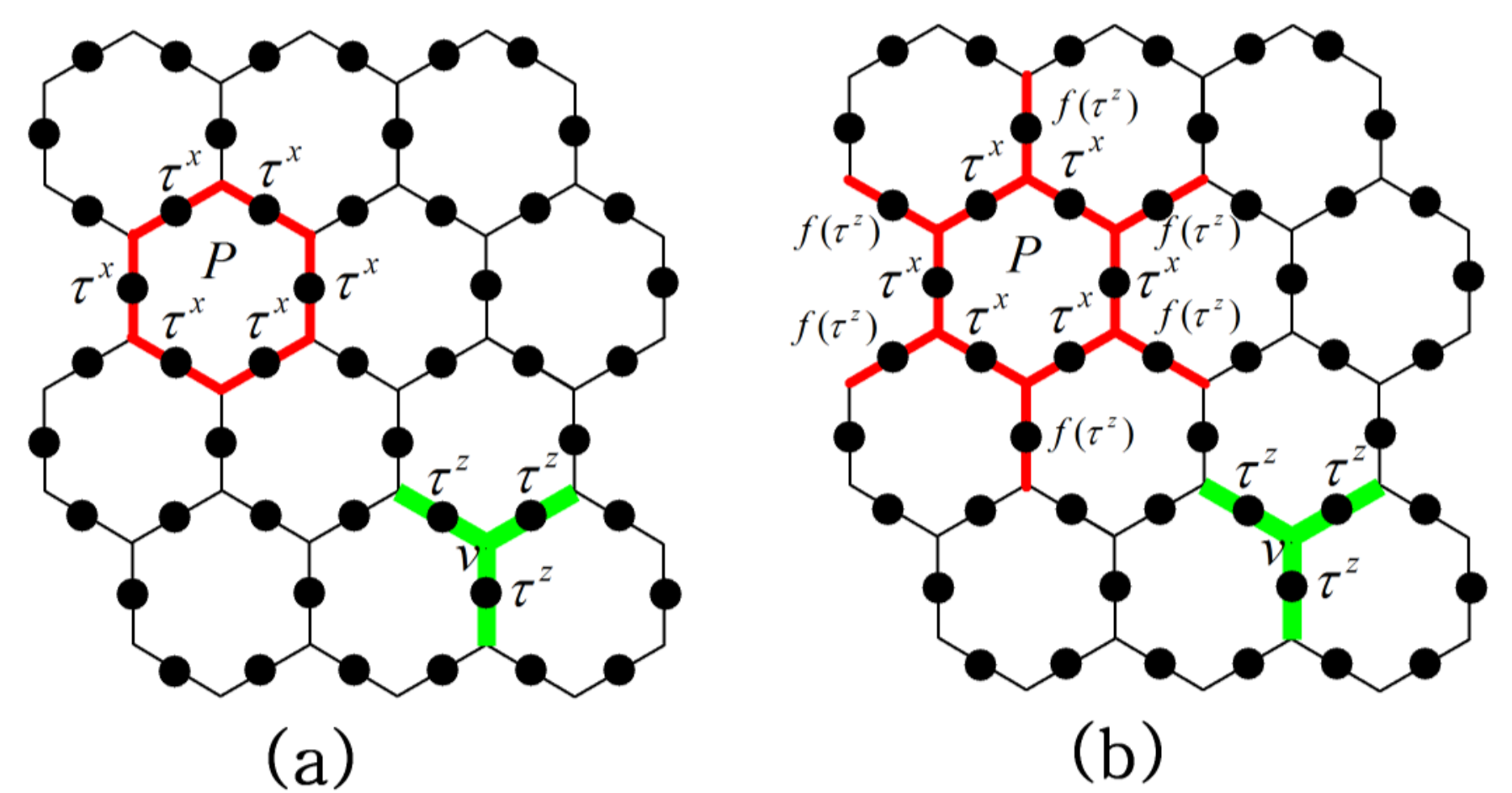
Here $\prod_{l\in p}\tau^{x}_{l}$ is the product of the $\tau^{x}_{l}$ around a plaquette $p$ and $\prod_{l\in v}\tau^{z}_{l}$ is the product of the $\tau^{z}_{l}$ around a vertex $v$. These two models are simplest examples of string-net models[40].

The ground state $|\Psi_{\mathrm{t.c.}}\rangle$ of $H_{\mathrm{t.c.}}$ is exactly known since all the plaquette terms and vertex terms commute with each other. The string language provides us with a very intuitive way to understand the ground state wave function: we interpret the $\tau^{z}_{l}=-1$ and $\tau^{z}_{l}=1$ states on a single link as the presence or absence of a string. (This string is literally an electric flux line in the $\mathbb{Z}_{2}$ gauge theory.) The appropriate low energy Hilbert space is made up of closed string states that satisfy $\prod_{l\in v}\tau^{z}_{l}=1$ at every vertex. The ground state is simply a superposition of all closed string states:

$\displaystyle|\Psi_{\mathrm{t.c.}}\rangle=\sum_{X\rm{closed}}|X\rangle,$

(3)

Such a model realizes the simplest topologically ordered state in 2D. If we put the ground state wave function Eq. (3) on a torus, there are four different topological sectors, characterized by even/odd number of large strings wrapping around a torus in both directions. Moreover, the $\mathbb{Z}_{2}$ electric charge $e$ can be described as the ends of a string, which are bosons and are created/annihilated in pairs.

$H_{\mathrm{d.s.}}$ is a less well-known model, which has the same number of ground state degeneracy on torus, but exhibits a different kind of topological order. The low energy Hilbert space of the model is again made up of closed string states. However, the ground state wavefunction of this model is very similar to the toric code wavefunction except that different closed string states are weighted by different phase factors:

$\displaystyle|\Psi_{\mathrm{d.s.}}\rangle=\sum_{X\rm{closed}}(-)^{n(X)}|X\rangle$

(4)

where $n$ is the number of closed loops in the closed-string state $X$. The $(-)^{n(X)}$ phase factor makes the $\mathbb{Z}_{2}$ electric charge(described as the ends of string) carry semion statistics.

The above two models can be mapped to $\mathbb{Z}_{2}$ gauge models and twisted $\mathbb{Z}_{2}$ gauge models on dual triangular lattices[27]. Edges of the triangular lattice are perpendicular to edges of the original honeycomb lattice. Spins on the edges are mapped accordingly. Centers of hexagonal plaquettes in the honeycomb lattice correspond to vertices of the triangular lattice. We put additional spins on these vertices. For each new spin, associate a gauge transformation

$\displaystyle W_{p}=\sigma_{p}^{x}\prod_{q}\mu_{pq}^{x}$

(5)

where $p$ labels a vertex in the triangular lattice and $pq$ labels the edge connecting $p$ and $q$, so that dimension of the physical Hilbert space remains the same. Operator mapping compatible with the gauge transformation is then found to be

$\displaystyle\tau_{l}^{z}=\sigma_{p}^{z}\sigma_{q}^{z}\mu_{pq}^{z},\quad\tau_{l}^{x}=\mu_{pq}^{x}.$

(6)

The resulting Hamiltonians reads (see Fig. 2)

	$$\displaystyle\begin{aligned} H_{0}=-\sum_{\langle pqr\rangle}\mu^{z}_{pq}\mu^{z}_{qr}\mu^{z}_{rp}-\sum_{p}\sigma_{p}^{x}O_{p}\\ H_{1}=-\sum_{\langle pqr\rangle}\mu^{z}_{pq}\mu^{z}_{qr}\mu^{z}_{rp}-\sum_{p}B_{p}O_{p}\end{aligned}$$
	$$\displaystyle O_{p}=\prod_{\langle pqr\rangle}\frac{1+\mu^{z}_{pq}\mu^{z}_{qr}\mu^{z}_{rp}}{2},\quad B_{p}=\sigma_{p}^{x}\prod_{\langle pqq^{\prime}\rangle}i^{\frac{1+\sigma_{q}^{z}\mu_{qq^{\prime}}^{z}\sigma_{q^{\prime}}^{z}}{2}}$$

where the product runs over six triangles adjacent to the vertex $p$. Apparently, $\mu_{pq}^{z}$ can be regarded as the $\mathbb{Z}_{2}$ gauge connection. Both $H_{0}$ and $H_{1}$ are invariant under the $\mathbb{Z}_{2}$ gauge transformation.

We now consider a system whose upper half plane is described by the toric code model and lower half plane is described by the doubled semion model. All local terms of the Hamiltonian commute with each other except on the domain wall. Denote the plaquette operators in the Hamiltonian Eq. (1) as

		$\displaystyle B^{\mathrm{t.c.}}_{p}=\prod_{l\in p}\tau_{l}^{x}$
		$\displaystyle B^{\mathrm{d.s.}}_{p}=\prod_{l\in p}\tau_{l}^{x}\prod_{l\in\text{legs of }p}i^{\frac{1+\tau_{l}^{z}}{2}}$		(7)

and label the plaquettes on the domain wall in a sequential order as shown in Fig. 3a. The nontrivial Hamiltonian algebra on the domain wall can be written as

		$\displaystyle\left(B^{\mathrm{t.c.}}_{n}\right)^{2}=1,\quad\left(B^{\mathrm{d.s.}}_{n}\right)^{2}=1$
		$\displaystyle\left[B^{\mathrm{t.c.}}_{m},B^{\mathrm{d.s.}}_{n}\right]=0,\quad\text{when~}\left|m-n\right|>1$
		$\displaystyle B^{\mathrm{t.c.}}_{n}B^{\mathrm{d.s.}}_{n\pm 1}=-B^{\mathrm{d.s.}}_{n\pm 1}B^{\mathrm{t.c.}}_{n}\tau_{n-1,n+1}^{z}\tau_{n\pm 1,n\pm 2}^{z}$		(8)

where $\tau_{m,n}^{z}$ denotes the spin operator on the edge in between plaquettes $m$ and $n$. Unfortunately, the above Hamiltonian algebra is very complicated and can not be solved in an easy way. On the other hand, this domain wall model and its operator algebra can be easily translated to the $\mathbb{Z}_{2}$ gauge models through mappings defined in the previous section (see Fig. 3b):

		$\displaystyle\left(\sigma_{n}^{x}\right)^{2}=1,\quad(B_{n})^{2}=1$
		$\displaystyle\left[\sigma_{m}^{x},B_{n}\right]=0,\quad\text{when~}\left|m-n\right|>1$
		$\displaystyle\sigma_{n}^{x}B_{n\pm 1}=-B_{n\pm 1}\sigma_{n}^{x}\sigma_{n\mp 1}^{z}\sigma_{n\pm 2}^{z}\mu_{n-1,n+1}^{z}\mu_{n\pm 1,n\pm 2}^{z}$		(9)

We would like to simplify the Hamiltonian algebra Eq. (9) in the low energy sector by choosing a convenient gauge and fix all spins on edges. The $\mathbb{Z}_{2}$ flux terms $-\mu^{z}_{pq}\mu^{z}_{qr}\mu^{z}_{rp}$ commute with all other terms in both $H_{0}$ and $H_{1}$, hence always represent an independent finite energy change. Therefore, we expect the low energy physics of a gapless domain wall to be entirely captured in the subspace where $\mu^{z}_{pq}\mu^{z}_{qr}\mu^{z}_{rp}=1$, i.e. no local $\mathbb{Z}_{2}$ flux. We will show later that the domain wall is indeed gapless. The simplest configuration with no local gauge flux is $\mu^{z}_{pq}\equiv 1$. Given any eigenstate of $\{\mu^{z}_{p}\}$ with no local gauge flux, the uniform $\mu^{z}_{pq}\equiv 1$ configuration can be achieved by applying gauge transformations if and only if there is no global gauge flux going through the domain wall, or equivalently in the string-net language, when there is no global string crossing the domain wall. We will henceforth assume this is the case and use the uniform gauge.

Under this uniform gauge, the domain wall Hamiltonian algebra simplifies to

		$\displaystyle\left(\sigma_{n}^{x}\right)^{2}=1,\quad(\bar{B}_{n})^{2}=1$
		$\displaystyle\left[\sigma_{m}^{x},\bar{B}_{n}\right]=0,\quad\text{when~}\left|m-n\right|>1$
		$\displaystyle\sigma_{n}^{x}\bar{B}_{n\pm 1}=-\bar{B}_{n\pm 1}\sigma_{n}^{x}\sigma_{n\mp 1}^{z}\sigma_{n\pm 2}^{z}$		(10)

Such a Hamiltonian algebra can naturally arise on the domain wall between the trivial and non-trivial $\mathbb{Z}_{2}$ SPT phases. The corresponding bulk Hamiltonians are simply those of the gauge models $H_{0}$, $H_{1}$ with only spins on vertices and without gauge fields on edges (Fig. 4)

	$$\displaystyle\bar{H}_{0}=-\sum_{p}\sigma_{p}^{x},\qquad\bar{H}_{1}=-\sum_{p}\bar{B}_{p}$$		(11)
	$$\displaystyle\bar{B}_{p}=\sigma_{p}^{x}\prod_{\langle pqq^{\prime}\rangle}i^{\frac{1+\sigma^{z}_{q}\sigma^{z}_{q^{\prime}}}{2}}.$$

where the product runs over all six triangles $\langle pqq^{\prime}\rangle$ containing $p$. Both systems have spin-flip $\mathbb{Z}_{2}$ global symmetry $S=\prod_{p}\sigma_{p}^{x}$ inherited from the gauge symmetry, and both have commuting local terms and unique ground states. Specifically, ground state wave functions are

	$$\displaystyle|\Psi_{0}\rangle=\sum_{\{\alpha_{p}\}}|\{\alpha_{p}\}\rangle$$
	$$\displaystyle|\Psi_{1}\rangle=\sum_{\{\alpha_{p}\}}(-1)^{N_{dw}}|\{\alpha_{p}\}\rangle$$		(12)

where $\{\alpha_{p}\}$ is a spin configuration in $\sigma_{p}^{z}$ eigenbasis with $\alpha_{p}=\uparrow$ or $\downarrow$, and $N_{dw}$ is the number of domain walls between spin up and down regions.

As shown in Ref. 27, these two spin models realize the only two short range entangled bosonic phases with onsite $\mathbb{Z}_{2}$ symmetry. We can, in fact, start from these two SPT models and follow the gauge coupling procedures specified in Ref. 27 to obtain the $\mathbb{Z}_{2}$ gauge models $H_{0}$, $H_{1}$. On the other hand, the domain wall models between the two SPT models $\bar{H}_{0}$ and $\bar{H}_{1}$ satisfy the Hamiltonian algebra Eq. (10) automatically.

The Hamiltonian algebra of the gauge-fixed flux free domain wall decouples from the bulk terms, so it can be realized on a purely 1+1D spin model. We can straightforwardly check that the following mapping to virtual spin operators $\{\bar{\tau}^{x}_{n},\bar{\tau}^{y}_{n},\bar{\tau}^{z}_{n}\}$ preserves this algebra Eq. (10)

	$\displaystyle\sigma_{n}^{x}$	$\displaystyle=\frac{1}{\sqrt{2}}\left(\bar{\tau}^{y}_{n}+\bar{\tau}^{z}_{n-1}\bar{\tau}^{x}_{n}\bar{\tau}^{z}_{n+1}\right)$
	$\displaystyle\bar{B}_{n}$	$\displaystyle=\frac{1}{\sqrt{2}}\left(\bar{\tau}^{y}_{n}-\bar{\tau}^{z}_{n-1}\bar{\tau}^{x}_{n}\bar{\tau}^{z}_{n+1}\right)$
	$\displaystyle\sigma^{z}_{n}$	$\displaystyle=\bar{\tau}^{z}_{n}$		(13)

In particular, we verify that

		$\displaystyle\sigma_{n}^{x}\bar{B}_{n+1}$
	$\displaystyle=$	$\displaystyle\frac{1}{2}\left(\bar{\tau}^{y}_{n+1}+\bar{\tau}^{z}_{n}\bar{\tau}^{x}_{n+1}\bar{\tau}^{z}_{n+2}\right)\left(\bar{\tau}^{y}_{n}-\bar{\tau}^{z}_{n-1}\bar{\tau}^{x}_{n}\bar{\tau}^{z}_{n+1}\right)$
	$\displaystyle=$	$\displaystyle-\frac{1}{2}\left(\bar{\tau}^{y}_{n+1}-\bar{\tau}_{n}^{z}\bar{\tau}^{x}_{n+1}\bar{\tau}_{n+2}^{z}\right)\bar{\tau}_{n+2}^{z}\bar{\tau}^{z}_{n-1}\left(\bar{\tau}^{z}_{n-1}\bar{\tau}^{x}_{n}\bar{\tau}^{z}_{n+1}+\bar{\tau}^{y}_{n}\right)$
	$\displaystyle=$	$\displaystyle-\bar{\tau}^{z}_{n-1}\bar{\tau}_{n+2}^{z}\bar{B}_{n+1}\sigma_{n}^{x}$		(14)

We further unitarily transform the operators with $U=\prod^{\prime}\bar{\tau}^{y}_{n}$, where the product runs over every other site on the domain wall. This makes all $\bar{B}_{n}$’s and $\sigma_{n}$’s take the same form and enhances translational symmetry of the effective Hamiltonian, which takes the final form

$\displaystyle H_{\mathrm{dw}}=-\frac{1}{\sqrt{2}}\sum_{n}\left(\bar{\tau}_{n}^{y}+\bar{\tau}_{n-1}^{z}\bar{\tau}_{n}^{x}\bar{\tau}_{n+1}^{z}\right)$

(15)

We will henceforth refer to this model as the Ising domain wall model. This model has a $\mathbb{Z}_{2}$ symmetry

$\displaystyle S_{\mathrm{dw}}=\prod_{n}\bar{\tau}^{x}_{n}\prod_{n}\exp\left[\frac{i\pi}{4}\left(\bar{\tau}^{z}_{n}\bar{\tau}^{z}_{n+1}-\bar{\tau}^{z}_{n}-1\right)\right],$

(16)

which we will show in Sec. III is indeed the $\mathbb{Z}_{2}$ symmetry inherited from the gauge symmetry in the bulk. This symmetry also acts as a self-dual transformation, as it transforms the two terms $\bar{\tau}^{y}_{n}$ and $\bar{\tau}^{z}_{n-1}\bar{\tau}^{x}_{n}\bar{\tau}^{z}_{n+1}$ into each other. We introduce an adjustable parameter $g$ into $H_{\mathrm{dw}}$ and transform this more general model with $S_{\mathrm{dw}}$:

	$$\displaystyle H_{\mathrm{dw}}(g)=-\frac{1}{\sqrt{2}}\sum_{n}\left(g\bar{\tau}^{y}_{n}+\bar{\tau}^{z}_{n-1}\bar{\tau}^{x}_{n}\bar{\tau}^{z}_{n+1}\right)$$		(17)
	$$\displaystyle S_{\mathrm{dw}}^{\dagger}H_{\mathrm{dw}}(g)S_{\mathrm{dw}}=gH_{\mathrm{dw}}(1/g)$$		(18)

We see that the spectrum of $H_{\mathrm{dw}}(g)$ and $H_{\mathrm{dw}}(1/g)$ is the same up to a factor of $g$, which makes $g=1$ a self-dual point. The spectrum of such a self-dual model is likely to be critical. On the other hand, since the flux free Hamiltonian algebra Eq. (10) is also realized as the domain wall between a trivial and a non-trivial $\mathbb{Z}_{2}$ SPT phases, it is natural to expect such a domain wall model to be gapless if the global $\mathbb{Z}_{2}$ symmetry is not spontaneously broken.

We now perform numerical calculations on the Ising domain wall model $H_{\mathrm{dw}}$ in Eq. (15). We show strong evidence that the model is indeed critical. More precisely, our numerical evidence shows that the low-energy physics is described by the $su(2)_{1}$ WZW theory, or equivalently the compactified free boson CFT at the self-dual radius.

We perform both exact diagonalization for small system size and loop-TNR calculation for larger system size. For comparison, we also perform numerical calculations on the spin-1/2 XXX Heisenberg chain

$\displaystyle H_{XXX}=\sum_{n}\left(\sigma^{x}_{n}\sigma^{x}_{n+1}+\sigma^{y}_{n}\sigma^{y}_{n+1}+\sigma^{z}_{n}\sigma^{z}_{n+1}\right),$

(19)

which is known to be described by the $su(2)_{1}$ WZW conformal field theory at low energy.

We first compute low energy spectra of both models $H_{\mathrm{dw}}$ and $H_{XXX}$ by exact diagonalization. In Fig. 5, the lowest eigenenergies of the two models on a periodic spin chain at the size of 30 sites are plotted against corresponding lattice momenta. Both models have a typical CFT excitation tower with linear dispersion, and an identification of low energy states between the two models is clear. Starting from the ground state, degeneracies of the first few energy levels are $\{1,3,1,6,6,\dots\}$ in both models. When computing lattice momenta, we use only three-site translations for the Ising domain wall model and two-site translations for the XXX model. Using a finer translational symmetry in either model would cause the unique excitation tower at $k=0$ to split into three/two towers at different momenta, making comparisons difficult.

The $su(2)_{1}$ WZW theory is equivalent to a free compactified boson at the self-dual radius. A general formula for scaling dimensions of the compactified free boson CFT is

$\displaystyle\Delta_{m,n}=\frac{1}{2}\left(\rho^{2}m^{2}+\frac{n^{2}}{\rho^{2}}\right),\quad m,n\in\mathbb{Z}.$

(20)

where $m,n$ label different primary fields and $\rho$ is the compactification radius (in our convention, $\rho=1$ is the self-dual radius). In addition to states with the above scaling dimensions, there are also states corresponding to the current operator as well as its powers and derivatives. The scaling dimensions of the latter states are all integers. More discussion on free compactified boson is given in Appendix C. At self-dual radius $\rho=1$, low lying scaling dimensions of all quasi-primaries are $\{0,0.5,1.0,1.5,2.0,2.5,\dots\}$ with degeneracies $\{1,4,6,8,17,28,\dots\}$. Finite size excitation energies should be proportional to scaling dimensions as $E_{i}=2\pi v\Delta_{i}/L$, but this correspondence can hardly be observed in our exact diagonalization result (Fig. 5). This large deviation from CFT prediction is well understood for the XXX model, where marginally irrelevant fields cause strong finite size effects that fall off only logarithmically with increasing system size[41]. We expect a similar logarithmic convergence for the Ising domain wall.

To access larger system size, we next use loop-TNR[38] to compute the central charge and scaling dimensions of both the Ising domain wall and the XXX model. Results are shown in Fig. 6. The system size grows exponentially with iteration steps in loop-TNR, hence the logarithmic convergence of the finite size effect is translated into a power law, which is indeed observed in Fig. 6 for both models. Even though full convergence cannot be reached before numerical errors drive the system away from the RG fixed point, we can still identify each scaling dimension’s corresponding exact values based on their trend, and recover the correct degeneracies in the expected convergence limit.

Finally, we deform the Ising domain wall model without breaking its anomalous global $\mathbb{Z}_{2}$ symmetry (16), and see how scaling dimensions change with the deformation. To find such a suitable deformation, it is easier to first make a unitary transformation

$\displaystyle U=\prod_{n}\exp\left[\frac{i\pi}{8}\left(\bar{\tau}^{z}_{n}-\bar{\tau}^{z}_{n}\bar{\tau}^{z}_{n+1}\right)\right]\prod_{n}\bar{\tau}^{x}_{n}.$

(21)

The transformed Hamiltonian can then be written as a special case of a more general class of Hamiltonians all sharing one $\mathbb{Z}_{2}$ symmetry:

$\displaystyle H^{\prime}_{\mathrm{dw}}(g)=\frac{1}{2}\sum_{n}\left[1-\bar{\tau}_{n-1}^{z}\bar{\tau}_{n+1}^{z}+g\left(\bar{\tau}_{n-1}^{z}+\bar{\tau}_{n+1}^{z}\right)\right]\bar{\tau}_{n}^{x}$

(22)

with

$\displaystyle S^{\prime}_{\mathrm{dw}}=\prod_{n}\bar{\tau}_{n}^{x}\prod_{n}\exp\left[\frac{i\pi}{4}\left(\bar{\tau}_{n}^{z}\bar{\tau}_{n+1}^{z}-1\right)\right]$

(23)

In particular, $H^{\prime}_{\mathrm{dw}}(g=1)$ is the transformed Ising domain wall model, and $H^{\prime}_{\mathrm{dw}}(g=0)$ is unitarily equivalent to the $XY$ model

	$$\displaystyle U^{\prime}=\prod_{n}\bar{\tau}^{x}_{4n}\bar{\tau}^{x}_{4n+1}\prod_{n}e^{\frac{i\pi}{4}\left(\bar{\tau}^{z}_{2n}\bar{\tau}^{z}_{2n+1}-\bar{\tau}^{z}_{2n}\right)}e^{-\frac{i\pi}{4}\bar{\tau}^{x}_{2n}}e^{\frac{i\pi}{4}\bar{\tau}^{y}_{2n+1}}$$
	$$\displaystyle U^{\prime{\dagger}}H^{\prime}_{\mathrm{dw}}(0)U^{\prime}=\sum_{n}\left(\bar{\tau}^{x}_{n}\bar{\tau}^{x}_{n+1}+\bar{\tau}^{y}_{n}\bar{\tau}^{y}_{n+1}\right)$$		(24)

which is known to realize the $\rho=\frac{1}{\sqrt{2}}$ compactified free boson CFT. We compute scaling dimensions of this deformed Ising domain wall model for $0\leq g\leq 1$, and find excellent agreement with compactified boson CFT with $\frac{1}{\sqrt{2}}\leq\rho\leq 1$ (Fig. 7). It is known that for a free boson CFT with $\rho\neq 0.5$, changing $\rho$ is the only relevant direction that preserves both conformal symmetry and $c=1$[42]. We have therefore rather conclusively shown that the Ising domain wall indeed realizes the compactified free boson CFT at self-dual radius.

The domain wall between the toric code and double semions can be alternatively viewed as the boundary of a stacking system of the two. It is then interesting to investigate the bulk properties of the stacking system and how they relate to the boundary domain wall.

We note that the toric code model has four types of anyons $1,e,m,f\equiv em$, where $e,m$ are bosons and the bound state $em$ is a fermion. While the double semion model also has four types of anyons $1,s,\bar{s},b\equiv s\bar{s}$, where $s$ and $\bar{s}$ are semions and the bound state $b$ is a boson. It is well known the toric code model admits a gapped boundary in general since we can condense the Lagrangian subset $(1,e)$ or $(1,m)$. Similarly, the double semion model also admits a gapped boundary since we can condense the Lagrangian subset $(1,b)$. Therefore, the stacking systems has sixteen types of anyons described by $(1,e,m,f)\otimes(1,s,\bar{s},b)$. In general, it also admits gapped boundary by condensing the Lagrangian subsets $(1,e)\otimes(1,b)=(1,e,b,eb)$ or $(1,m)\otimes(1,b)=(1,m,b,mb)$.

Then what is the mechanism that protects the gapless nature of the domain wall? What makes the domain wall model so special such that it is an $su(2)_{1}$ WZW CFT? For the first question, a quick answer can be achieved by ungauging the $\mathbb{Z}_{2}$ gauge symmetry in both models and mapping the domain wall model back to a special boundary of $\mathbb{Z}_{2}$ SPT phase. Since both toric code model and double semion model can be regarded as the deconfinement phase of $\mathbb{Z}_{2}$ gauge theory, their domain wall is also in the deconfinement phase where the $\mathbb{Z}_{2}$ symmetry can not be spontaneously broken. Thus, the corresponding ungauged domain wall model must be a $\mathbb{Z}_{2}$ SPT boundary without spontaneously symmetry broken, which must be gapless. (It is well known that the boudary of $2+1$D SPT phase must be either gapless or symmetry breaking.) A more rigorous argument can be achieved by regarding the domain wall model as a specific boundary of toric code and double semion stacking systems with $eb$ condensation while $e$ and $b$ are not condensed individually. Clearly, such a condition will exclude the condensation of Lagrangian subset $(1,e,b,eb)$ or $(1,m,b,mb)$ and protect the gapless nature of the boundary. Very recently, a more precise mathematical language, namely, the categorical symmetry[43] is introduced to understand such a special boundary and our lattice model construction can be regarded as an explicit realization of the maximal categorical symmetry for ground state wevefunctions.

The second problem is much more subtle, and we need to analyze the anyon content for the stacking model after condensing $eb$. Since all the anyons with nontrivial statistics with $eb$ are confined, the remaining anyons are consisting of one boson $b$ (which is identified to $e$) and two semions $ms,m\bar{s}$ (which are identified with $f\bar{s},fs$). Together with the identity particle, we end up with a new double semion model with four anyons $1,b,ms,m\bar{s}$, whose corresponding $K$ matrix reads:

$\displaystyle K=\begin{bmatrix}2&0\\ 0&-2\end{bmatrix}$

(25)

Apparently, if it is not allowed to condense $b$ in the deconfinement phase, there is no Lagrangian subset can be condensed in the above theory and we will end up with a $c=1$ CFT. It is well known that the above K-matrix describes two layers of filling fraction $\nu=1/2$ bosonic Laughlin states with opposite chirality. Since the edge theory of $\nu=1/2$ bosonic Laughlin state is described by the chiral $su(2)_{1}$ WZW model, it is quite natural that the domain wall model can be described as the stacking of two chiral $su(2)_{1}$ WZW models with opposite chirality, if we assume there is no interactions between the left and right movers. However, we stress that the emergence of $SU(2)$ symmetry in the above gapless domain wall model is accidental and it does not apply to generic $\mathbb{Z}_{2}$ gapless domain wall model preserving the anomalous $\mathbb{Z}_{2}$ symmetry Eq. (23). Physically, this is because the interactions between left and right movers always exist in generic $\mathbb{Z}_{2}$ gapless domain wall models, which makes the radius $\rho$ deviate from $1$, e.g., Hamiltonian Eq. (22) with $g\neq 1$. We will discuss more details in next section.

We first briefly review the construction of a lattice model realizing a 2D SPT phase with finite on-site symmetry $G$[4].

We define our model on a triangular lattice. Each vertex is associated with a $\left|G\right|$-dim Hilbert space where local basis states $|g\rangle$ are labeled by group elements $g\in G$. The model is constructed with a branching structure on the lattice and a $3$-cocycle in the group cohomology $\mathcal{H}^{3}(G,U(1))$. A branching structure is an assignment of arrows on all edges of the lattice such that there is no local oriented loop, which defines a natural ordering of vertices for each triangle. A $3$-cocycle, for our purpose, is a function $\nu:G^{4}\to U(1)$ that satisfies two conditions

	$$\displaystyle\nu(gg_{0},gg_{1},gg_{2},gg_{3})=\nu(g_{0},g_{1},g_{2},g_{3})$$		(26a)
	$$\displaystyle\frac{\nu(g_{1},g_{2},g_{3},g_{4})\nu(g_{0},g_{1},g_{3},g_{4})\nu(g_{0},g_{1},g_{2},g_{3})}{\nu(g_{0},g_{2},g_{3},g_{4})\nu(g_{0},g_{1},g_{2},g_{4})}=1$$		(26b)

for any $g,g_{i}\in G$. Two $3$-cocycles $\nu,\nu^{\prime}$ are considered equivalent if they only differ by a $3$-coboundary $\lambda$, i.e. $\nu^{\prime}=\nu\lambda$. A $3$-coboundary is a function $\lambda:G^{4}\to U(1)$ that satisfies

	$$\displaystyle\lambda(g_{0},g_{1},g_{2},g_{3})=\frac{\mu(g_{1},g_{2},g_{3})\mu(g_{0},g_{1},g_{3})}{\mu(g_{0},g_{2},g_{3})\mu(g_{0},g_{1},g_{2})}$$
	$$\displaystyle\mu(gg_{0},gg_{1},gg_{2})=\mu(g_{0},g_{1},g_{2})$$		(27)

The choice of coboundary can be thought of as a gauge freedom for cocycles. Equivalent classes of $3$-cocycles form the third group cohomology $\mathcal{H}^{3}(G,U(1))$, which itself is an Abelian group. A more detailed introduction to group cohomology can be found in Appendix A.

Define a unitary transformation on the triangular lattice with a branching structure (Fig. 8)

$\displaystyle U_{\nu}|\{g_{i}\}\rangle=\prod_{\{pqr\}}\nu^{s_{pqr}}(g_{p},g_{q},g_{r},g^{*})|\{g_{i}\}\rangle$

(28)

where $g^{*}$ is a fixed group element, the product runs over all triangles labeled by their three vertices $pqr$ ordered according to the branching structure, and $s_{pqr}=\pm 1$ if the triangle has anticlockwise/clockwise orientation respectively. The Hamiltonian is defined as

	$$\displaystyle H_{\nu}=-\sum_{p}H_{p},\quad H_{p}=U_{\nu}|\phi_{p}\rangle\langle\phi_{p}|U_{\nu}^{\dagger}$$
	$$\displaystyle|\phi_{p}\rangle=\sum_{g_{p}\in G}|g\rangle.$$		(29)

Although $U_{\nu}$ acts on the entire lattice, each term of the Hamiltonian acts non-trivially only on seven neighboring sites centered at $p$. Explicitly, with a branching structure as shown in Fig. 8,

		$\displaystyle\langle g_{p}^{\prime},g_{1}g_{2}g_{3}g_{4}g_{5}g_{6}|H_{p}|g_{p},g_{1}g_{2}g_{3}g_{4}g_{5}g_{6}\rangle$
	$\displaystyle=$	$\displaystyle\frac{\nu(g_{4},g_{5},g_{p},g_{p}^{\prime})\nu(g_{5},g_{p},g_{p}^{\prime},g_{6})\nu(g_{p},g_{p}^{\prime},g_{6},g_{1})}{\nu(g_{p},g_{p}^{\prime},g_{2},g_{1})\nu(g_{3},g_{p},g_{p}^{\prime},g_{2})\nu(g_{4},g_{3},g_{p},g_{p}^{\prime})}.$		(30)

This expression has been simplified using the cocycle condition (26b). All local terms commute, so the model is exactly solvable. It has a unique ground state

$\displaystyle|\Psi_{\mathrm{GS}}\rangle=\sum_{\{g_{p}\}}U_{\nu}|\{g_{p}\}\rangle.$

(31)

Both the Hamiltonian and the ground state have the $G$ symmetry $\{|g_{p}\rangle\}\to\{|gg_{p}\rangle\}$. Models realize distinct SPT phases if and only if they are defined by inequivalent $3$-cocycles.

We now use the construction in the previous section to derive domain wall models between different SPT phases with the same symmetry $G$.

Consider a system on a triangular lattice with the Hamiltonian

$\displaystyle H=-\sum_{p\in\{\circ\}}H^{a}_{p}-\sum_{p\in\{\bullet\}}H^{b}_{p}$

(32)

where $\{\circ\}$ and $\{\bullet\}$ denote vertices in the upper and lower half plane respectively (Fig. 9). Each local term $H_{p}^{a,b}$ acts on seven neighboring sites centered at $p$. $H_{p}^{a}$ and $H_{p}^{b}$ are defined similarly by Eq. (29), but use two inequivalent cocycles $\nu_{a},\nu_{b}$. All $H^{a}_{p}$’s commute and all $H^{b}_{p}$’s commute, leaving the domain wall as the only nontrivial part of the system.

To explicitly decouple the domain wall from the bulk, we consider the unitary transformation

	$\displaystyle U_{ab}=$	$\displaystyle\prod_{\{pqr\}\in\mathcal{A}}\nu_{a}^{s_{pqr}}(g_{p},g_{q},g_{r},g^{*})$
		$\displaystyle\cdot\prod_{\{p^{\prime}q^{\prime}r^{\prime}\}\in\mathcal{B}}\nu_{b}^{s_{p^{\prime}q^{\prime}r^{\prime}}}(g_{p^{\prime}},g_{q^{\prime}},g_{r^{\prime}},g^{*})$		(33)

where $\mathcal{A}$ and $\mathcal{B}$ are regions on the lattice, as shown in Fig. 9, that mostly represent upper and lower half planes respectively. It changes local terms in the bulk into trivial one body interaction, leaving the domain wall explicitly decoupled. On the domain wall, the Hamiltonian transforms into

	$$\displaystyle\begin{aligned} U_{ab}^{\dagger}H^{a}_{p}U_{ab}&=\sum_{g\in G}|gg_{p}\rangle\langle g_{p}|\,\frac{\nu^{s_{ijk}}_{ab}(g_{i},g_{j},g_{k},g^{*})}{\nu^{s_{ijk}}_{ab}(g_{i},gg_{j},g_{k},g^{*})},\\ U_{ab}^{\dagger}H^{b}_{p}U_{ab}&=\sum_{g\in G}|gg_{p}\rangle\langle g_{p}|\,\frac{\nu^{s_{ijk}}_{ab}(g_{i},gg_{j},g_{k},g^{*})}{\nu^{s_{ijk}}_{ab}(g_{i},g_{j},g_{k},g^{*})},\end{aligned}$$
	$$\displaystyle\nu_{ab}\equiv\nu_{a}^{-1}\nu_{b}.$$

$i,j,k$ label a triangle whose top or bottom vertex is $p$, while which vertex each of them represents is assigned according to the branching structure (Fig. 9). Due to the group structure of group cohomology $\mathcal{H}^{3}(G,U(1))$, we see that the domain wall is defined only by one $3$-cocycle $\nu_{ab}$ rather than two.

In general, different branching structures lead to different domain wall models, and $H_{p}^{a,b}$’s can be different from one another. For concreteness, we will mostly focus on the specific branching structure shown in Fig. 9. This branching structure is particularly nice, since it gives us a fully translational invariant domain wall. The corresponding Hamiltonian reads

	$$\displaystyle H=-\sum_{n}H_{n},$$
	$$\displaystyle\begin{aligned} &\langle g^{\prime}_{n},g_{n-1}g_{n+1}|H_{n}|g_{n},g_{n-1}g_{n+1}\rangle\\ =&\frac{\nu_{ab}(g_{n+1},g^{\prime}_{n},g_{n-1},g^{*})}{\nu_{ab}(g_{n+1},g_{n},g_{n-1},g^{*})}.\end{aligned}$$

Its effective anomalous symmetry operator can also be computed

$\displaystyle S_{g}|\{g_{n}\}\rangle=\prod_{n}\nu_{ab}^{-1}(g_{n+1},g_{n},g^{-1}g^{*},g^{*})|\{gg_{n}\}\rangle.$

(34)

Now we have obtained a general domain wall model of 2D bosonic SPT phases. To construct an explicit model, we only need to find explicit expression of group $3$-cocycles.

It is no coincidence that both $\mathbb{Z}_{N}$ gauge theories and SPT phases in 2+1D are classified by the group cohomology $\mathcal{H}^{3}(\mathbb{Z}_{N},U(1))\cong\mathbb{Z}_{N}$. We note that string-net realizations of all $N$ distinct $\mathbb{Z}_{N}$ gauge theories can be constructed[44], and lattice models exist for any SPT phases with finite on-site symmetry[4].

The formula of $\mathbb{Z}_{N}$ $3$-cocycles is well-known[45]

	$$\displaystyle\nu_{3}(g_{0},g_{1},g_{2},g_{3})=\exp\left[i\frac{2\pi k}{N^{2}}g_{10}\left(g_{21}+g_{32}-g_{31}\right)\right]$$		(35)
	$$\displaystyle g_{ij}\equiv(g_{i}-g_{j})~\mathrm{mod}~N$$
	$$\displaystyle g_{i},k\in\{0,1,\dots,N-1\}$$

where $g_{i}$ labels a group element and $k$ labels the $N$ different classes of $3$-cocycles in $\mathcal{H}^{3}(\mathbb{Z}_{N},U(1))\cong\mathbb{Z}_{N}$. Using this formula in Eq. (III.2), we can define a $\mathbb{Z}_{N}$ domain wall model that is labeled by $(N,k)$. Hamiltonians given by $(N,k)$ and $(N,N-k)$ are related by complex conjugation, therefore there are effectively only $\lfloor N/2\rfloor$ distinct nontrivial domain wall models for a given $N$.

References

- [1] X. Chen, Z.-C. Gu, and X.-G. Wen, “Complete classification of one-dimensional gapped quantum phases in interacting spin systems,” Phys. Rev. B 84, 235128 (2011a).
- [2] X. Chen, Z.-C. Gu, and X.-G. Wen, “Classification of gapped symmetric phases in one-dimensional spin systems,” Phys. Rev. B 83, 035107 (2011b).
- [3] N. Schuch, D. Pérez-García, and I. Cirac, “Classifying quantum phases using matrix product states and projected entangled pair states,” Phys. Rev. B 84, 165139 (2011).
- [4] Xie Chen, Zheng-Cheng Gu, Zheng-Xin Liu, and Xiao-Gang Wen, “Symmetry protected topological orders and the group cohomology of their symmetry group,” Phys. Rev. B 87, 155114 (2013).
- [5] Xiao-Gang Wen, “Construction of bosonic symmetry-protected-trivial states and their topological invariants via nonlinear models,” Phys. Rev. B 91, 205101 (2015).
- [6] Zheng-Cheng Gu, Zhenghan Wang, and Xiao-Gang Wen, “Classification of two-dimensional fermionic and bosonic topological orders,” Phys. Rev. B 91, 125149 (2015).
- [7] Zheng-Cheng Gu and Xiao-Gang Wen, “Symmetry-protected topological orders for interacting fermions: fermionic topological nonlinear models and a special group supercohomology theory,” Phys. Rev. B 90, 115141 (2014).
- [8] A. Kapustin, R. Thorngren, A. Turzillo, and Z. Wang, “Fermionic Symmetry Protected Topological Phases and Cobordisms,” arXiv e-prints (2014), arXiv:1406.7329 .
- [9] D. S. Freed, “Short-range entanglement and invertible field theories,” arXiv e-prints (2014), arXiv:1406.7278 .
- [10] M. Cheng, Z. Bi, Y.-Z. You, and Z.-C. Gu, “Towards a Complete Classification of Symmetry-Protected Phases for Interacting Fermions in Two Dimensions,” arXiv e-prints (2015), arXiv:1501.01313 .
- [11] Qing-Rui Wang and Zheng-Cheng Gu, “Towards a complete classification of fermionic symmetry protected topological phases in 3D and a general group supercohomology theory,” arXiv e-prints (2017), arXiv:1703.10937 .
- [12] Davide Gaiotto and Theo Johnson-Freyd, “Symmetry Protected Topological phases and Generalized Cohomology,” arXiv e-prints (2017), arXiv:1712.07950 .
- [13] M. Barkeshli, P. Bonderson, M. Cheng, and Z. Wang, “Symmetry, Defects, and Gauging of Topological Phases,” ArXiv e-prints (2014), arXiv:1410.4540 .
- [14] T. Lan, L. Kong, and X.-G. Wen, “Classification of 2+1D topological orders and SPT orders for bosonic and fermionic systems with on-site symmetries,” ArXiv e-prints (2016), arXiv:1602.05946 .
- [15] Lokman Tsui, Fa Wang, and Dung-Hai Lee, “Topological versus Landau-like phase transitions,” arXiv e-prints (2015), arXiv:1511.07460 .
- [16] Lokman Tsui, Yen-Ta Huang, Hong-Chen Jiang, and Dung-Hai Lee, “The phase transitions between bosonic topological phases in D, and a constraint on the central charge for the critical points between bosonic symmetry protected topological phases,” Nuclear Physics, B 919, 470 (2017).
- [17] F. A. Bais and J. K. Slingerland, “Condensate-induced transitions between topologically ordered phases,” Phys. Rev. B 79, 045316 (2009).
- [18] A. Kitaev and L. Kong, “Models for Gapped Boundaries and Domain Walls,” Communications in Mathematical Physics 313, 351–373 (2012), arXiv:1104.5047 .
- [19] Michael Levin, “Protected edge modes without symmetry,” Phys. Rev. X 3, 021009 (2013).
- [20] L.-Y. Hung and Y. Wan, “Symmetry-enriched phases obtained via pseudo anyon condensation,” International Journal of Modern Physics B 28, 1450172 (2014), arXiv:1308.4673 .
- [21] Tian Lan, Juven C. Wang, and Xiao-Gang Wen, “Gapped domain walls, gapped boundaries, and topological degeneracy,” Phys. Rev. Lett. 114, 076402 (2015).
- [22] Throughout the whole paper, we will regard vacuum as a trivial topological state. Thus, the boundary of a topological state can be regarded as a special kind of domain wall.
- [23] M. Z. Hasan and C. L. Kane, “Colloquium : Topological insulators,” Rev. Mod. Phys. 82, 3045–3067 (2010).
- [24] X.-L. Qi and S.-C. Zhang, “Topological insulators and superconductors,” Rev. Mod. Phys. 83, 1057–1110 (2011).
- [25] Y.-M. Lu and A. Vishwanath, “Theory and classification of interacting integer topological phases in two dimensions: A chern-simons approach,” Phys. Rev. B 86, 125119 (2012).
- [26] M. Levin and A. Stern, “Classification and analysis of two-dimensional abelian fractional topological insulators,” Phys. Rev. B 86, 115131 (2012).
- [27] Michael Levin and Zheng-Cheng Gu, “Braiding statistics approach to symmetry-protected topological phases,” Phys. Rev. B 86, 115109 (2012).
- [28] Xie Chen and Xiao-Gang Wen, “Chiral symmetry on the edge of 2d symmetry protected topological phases,” Phys. Rev. B 86, 235135 (2012).
- [29] Zheng-Xin Liu and Xiao-Gang Wen, “Symmetry protected spin quantum hall phases in 2-dimensions,” Phys. Rev. Lett. 110, 067205 (2013).
- [30] Edward Witten, “Quantum field theory and the jones polynomial,” Comm. Math. Phys. 121, 351–399 (1989).
- [31] Gerard ’t Hooft, “Dimensional reduction in quantum gravity,” arXiv preprint gr-qc/9310026 (1993).
- [32] Leonard Susskind, “The world as a hologram,” J. Math. Phys. 36, 6377–6396 (1995).
- [33] Gregory Moore and Nathan Seiberg, “Classical and quantum conformal field theory,” Comm. Math. Phys. 123, 177–254 (1989a).
- [34] B. I. Halperin, “Statistics of quasiparticles and the hierarchy of fractional quantized hall states,” Phys. Rev. Lett. 52, 2390–2390 (1984).
- [35] Daniel Arovas, J. R. Schrieffer, and Frank Wilczek, “Fractional statistics and the quantum hall effect,” Phys. Rev. Lett. 53, 722–723 (1984).
- [36] Alexei Kitaev, “Anyons in an exactly solved model and beyond,” Ann. Phys. 321, 2 – 111 (2006), january Special Issue.
- [37] Vladimir G. Turaev, “Modular categories and 3-manifold invariants,” Int. J. Mod Phys B 06, 1807–1824 (1992).
- [38] Shuo Yang, Zheng-Cheng Gu, and Xiao-Gang Wen, “Loop optimization for tensor network renormalization,” Phys. Rev. Lett. 118, 110504 (2017).
- [39] A.Yu. Kitaev, “Fault-tolerant quantum computation by anyons,” Ann. Phys. 303, 2 – 30 (2003).
- [40] Michael A. Levin and Xiao-Gang Wen, “String-net condensation: a physical mechanism for topological phases,” Phys. Rev. B 71, 045110 (2005).
- [41] I Affleck, D Gepner, H J Schulz, and T Ziman, “Critical behaviour of spin-s heisenberg antiferromagnetic chains: analytic and numerical results,” J. Phys. A 22, 511 (1989).
- [42] P Ginsparg, “Curiosities at c= 1,” Nucl. Phys. B 295, 153–170 (1988).
- [43] Wenjie Ji and Xiao-Gang Wen, “Categorical symmetry and non-invertible anomaly in symmetry-breaking and topological phase transitions,” arXiv e-prints (2019), arXiv:1912.13492 .
- [44] Chien-Hung Lin and Michael Levin, “Generalizations and limitations of string-net models,” Phys. Rev. B 89, 195130 (2014).
- [45] Gregory Moore and Nathan Seiberg, “Classical and quantum conformal field theory,” Communications in Mathematical Physics 123, 177–254 (1989b).
- [46] Pasquale Calabrese and John Cardy, “Entanglement entropy and quantum field theory,” J. Stat. Mech. Theory Exp. 2004, P06002 (2004a).
- [47] Steven R White, “Density matrix formulation for quantum renormalization groups,” Phys. Rev. Lett. 69, 2863 (1992).
- [48] Steven R White, “Density-matrix algorithms for quantum renormalization groups,” Phys. Rev. B 48, 10345 (1993).
- [49] Frank Verstraete, Diego Porras, and J Ignacio Cirac, “Density matrix renormalization group and periodic boundary conditions: A quantum information perspective,” Phys. Rev. Lett. 93, 227205 (2004).
- [50] Masuo Suzuki, “Transfer-matrix method and monte carlo simulation in quantum spin systems,” Physical Review B 31, 2957 (1985).
- [51] Xiao-Gang Wen, “Topological orders and edge excitations in fractional quantum hall states,” Adv. Phys. 44, 405–473 (1995).
- [52] Yuting Hu, Yidun Wan, and Yong-Shi Wu, “Twisted quantum double model of topological phases in two dimensions,” Physical Review B 87, 125114 (2013).
- [53] V. Zauner-Stauber, L. Vanderstraeten, M. T. Fishman, F. Verstraete, and J. Haegeman, “Variational optimization algorithms for uniform matrix product states,” Phys. Rev. B 97, 045145 (2018).
- [54] Laurens Vanderstraeten, Jutho Haegeman, and Frank Verstraete, “Tangent-space methods for uniform matrix product states,” SciPost Phys. Lect. Notes , 7 (2019).
- [55] F. Verstraete, V. Murg, and J.I. Cirac, “Matrix product states, projected entangled pair states, and variational renormalization group methods for quantum spin systems,” Advances in Physics 57, 143–224 (2008).
- [56] N. Schuch, “Condensed matter applications of entanglement theory,” arXiv:1306.5551 (2013).
- [57] Bruno Nachtergaele, “The spectral gap for some spin chains with discrete symmetry breaking,” Communications in Mathematical Physics 175, 565–606 (1996).
- [58] Pasquale Calabrese and John Cardy, “Entanglement entropy and quantum field theory,” Journal of Statistical Mechanics: Theory and Experiment 2004, P06002 (2004b).
- [59] Tian Lan, Liang Kong, and Xiao-Gang Wen, “Classification of bosonic topological orders: The case when pointlike excitations are all bosons,” Phys. Rev. X 8, 021074 (2018).
- [60] It is common to define -cochains as an arbitrary function from to . Our definition involves one more group element and an constraint on the function, and is essentially equivalent. Such a definition, although with redundancy, allows more convenient definitions and intuitive geometric interpretations of many of the algebraic objects defined later.
- [61] P. Francesco, P. Mathieu, and D. Senechal, Conformal Field Theory (Island Press, 1996).
- [62] Masuo Suzuki, “Relationship between d-dimensional quantal spin systems and (d+ 1)-dimensional ising systems: Equivalence, critical exponents and systematic approximants of the partition function and spin correlations,” Progress of theoretical physics 56, 1454–1469 (1976).
- [63] F Woynarovich, H-P Eckle, and TT Truong, “Non-analytic finite-size corrections in the one-dimensional bose gas and heisenberg chain,” Journal of Physics A: Mathematical and General 22, 4027 (1989).
- [64] Roman Orus and Guifre Vidal, “Infinite time-evolving block decimation algorithm beyond unitary evolution,” Physical Review B 78, 155117 (2008).