High Dimensional Spaces, Deep Learning and Adversarial ExamplesThanks: Email: simantdube@iitdalumni.com

Suppose one can perturb images very slightly to get adversarial examples and we were to bound this perturbation amount. An interesting question to ask is that given an image how probable it is to be able to perturb it within this bound and successfully get an adversarial example. For that, we first need the following Lemma.

We have straightforward corollary.

See Figure 3. Note that we can not conclude yet that expectation of $\left\|P(x)\right\|$ tends to 0 as $n$ approaches $\infty$ since we don’t know how radius $R$ of image manifold will increase with $n$. There are two cases.

1. (1)

   For 8-bit images, $B\subset[0,255]^{n}$ and is surrounded by a hypercube of diameter $255{\sqrt{n}}$. Thus, $R=O(\sqrt{n})$, and $\mathbb{E}(\left\|P(x)\right\|)$ shrinks to 0.

2. (2)

   For idealized images with arbitrary real pixel values, $B\subset\mathbb{R}^{n}$. See Section 4 that $\mathbb{E}(\left\|P(x)\right\|)$ does approach 0 for natural image manifolds.

Now we present the main result on adversarial examples. We first define concept of radius of a manifold.

Definition: Let $M\subset\mathbb{R}^{n}$ be an $n$-dimensional bounded manifold with finite volume. Then, its radius is

The diameter of the manifold, which is maximum pairwise distance, can be viewed as dynamic range of the corresponding image class. We want to bound the perturbation image relative to the radius. See Figure 4.

For $k$-bit images, $M\subset[0,2^{k}-1]^{n}$ and is surrounded by a hypercube of diameter of the order of ${\sqrt{n}}$. Thus, $R(M)=O(\sqrt{n})$. Therefore we have the following theorem.

Note that for the proof to work, we implicitly require that each positive image manifold is surrounded completely by its complement which will be the case if it is compact and the space is $\mathbb{R}^{n}$. For 8-bit images the total space in $[0,255]^{n}$ and as long as the positive manifolds are surrounded by their respective complements so that one can move out of the surfaces into the complement regions, proof will hold.

In Section 3 of the reference [10], it is argued that even simple linear models can suffer from adversarial negatives and problem in this argument has been independently highlighted earlier in [28]. The authors consider a simple linear model $w^{T}x$. Let $y=x+p$ be the adversarial negative with $p$ being the perturbation. See Figure 6.

Then,

In [10], $L_{\infty}$-norm of perturbation is constrained to a small value $\epsilon$ which is fixed to be the smallest greyness granularity, which is 1/255 of the dynamic range for 8-bit images. It is first argued that if $m$ is the average magnitude of coefficients of the weight vector $w$ and we choose $p^{\prime}=\epsilon\;{\rm sign}(w)$ to be closely aligned with $w$, then for $n$ dimensions, $w^{T}p^{\prime}=\epsilon mn$ will increase with $n$ to reach any target which will push the point on the other side of the decision hyperplane. We want $\epsilon mn$ to reach activation level to be negative of $w^{T}x$. It is argued in [10] that this is possible with increasing $n$. With increasing $n$, $w^{T}x$ also increases because $w$ and $x$ increase in their magnitudes as they have more elements in higher dimensional spaces. Therefore if we keep $L_{\infty}$-norm of perturbation constrained as in [10] to some small $\epsilon$, we can not generate adversarial examples using this argument for the linear model. In order to generate adversarial examples, we will have to set $L_{\infty}$-norm constraint to a higher value which will depend on the distance of $x$ from the decision boundary. But then there is no upper bound on the max norm due to fact that there is no upper bound on the distance of feature vector to the decision hyperplane. Even if we constrain the feature value range to be finite, such as [0,255] for 8-bit images, even then the distances can be fairly large in general case. Therefore, the generalization of the argument in [10] to deep networks is invalid.

Therefore, we can state the following.

At the same time, Theorem 3 in this paper will hold for all bounded manifolds. This is because image manifolds are assumed to be bounded and surrounded by their complement. As $n$ increases, the surface increases rapidly having more volume close to it, thereby bringing points closer to some surface where adversarial examples exist. The size of the manifold also increases and therefore the perturbation bound in Theorem 3 is expressed relative to this size. The size of the manifold does not increase that fast, and therefore perturbations become smaller even in absolute sense. This will also hold if the manifold is bounded from all sides by hyperplanes as a special case as shown in Figure 6. Deep networks perform this piecewise linear approximation of functions with ReLU activation, see [17], so our results apply to deep networks as a special case.

We adopt a related but different approach and use results from theory of random polynomials which give explicit bounds on number of critical points. In order to understand this well we will bound the number of saddle points and that of local minima by approximating loss surfaces, also referred to as optimization landscapes, with polynomials. For polynomial approximation of deep networks, see [14, 20] where ReLU is approximated by a polynomial and results on singularity of the Hessian are derived for overparameterized systems.

Key observation is that all the operations used in deep learning are continuous even though they may not be differentiable.

The continuity of functions is obvious for convolution layers, fully connected layers and differentiable loss functions. This is true of nonlinear layers such as ReLU and Max Pooling. Though they are not differentiable but they are continuous as their graphs don’t have breaks for continuous inputs. ReLU is piecewise linear. To see immediately how ReLU activation layer can be approximated by a polynomial, notice that it can be written as follows

in terms of absolute function which is known to have polynomial approximation. Max pooling is continuous for continuous inputs. Smooth versions of max are well-known. Notice that max can be expressed as follows

In fact, we have two kinds of polynomials:

• •

  Optimization Landscape Polynomials. We fix the image pixel values. Neural networks parameters are variables.

• •

  Image Polynomials. We fix the neural network parameters. Image pixel values are variables.

In both cases, we will have a very large polynomial. The degree of the polynomial goes up as layers in the network increase. As number of network parameters and image resolution go up, then the number of variables goes up.

In this section, we are concerned with optimization landscape polynomials. In Section 4, we will discuss image polynomials.

What can we say about number of saddle points and that of local minima of deep network polynomials? Since deep learning is a practical field, one will have to make assumptions based on empirically derived statistics on the coefficients of the polynomials based on particular applications. One will have to endow the space of deep network polynomials with a probability measure in order to derive mathematical results. We make use of results from theory of random polynomials endowed with Gaussian probability measure with certain assumptions on variances, see [6, 5], which provides evidence why deep learning works well in practice.

For proof, see [6, 5]. This result shows that most large random polynomials have only saddle points and local minima become increasingly rare. Assuming this result holds for most practical problems solved by deep learning, this implies that the number of local minima becomes arbitrarily small compared to number of saddle points as the resolution of images and size and depth of deep networks increase. The probability that all eigen values of the Hessian matrix of these polynomials are positive falls off very rapidly [5].

Under the assumption that the loss surfaces of deep neural networks are normal random polynomials as in [6, 5], we can state the following.

It has been shown in [3, 4, 7], both theoretically under certain assumptions as well as empirically, that the local minima are concentrated towards the bottom of the optimization landscape. Therefore during SGD we are likely to encounter local minima only towards the end of training which correspond to good enough solutions to practical problems. Earlier in the training, it is quite likely that slowing down is occuring because of a saddle point.

The above results also indicate why SGD and various tricks and techniques work in deep learning. Assume for a particular minibatch of training images, the deep network is at local minima or saddle point. As new minibatches arrive with their varying image statistics, optimization landscape changes and it becomes less likely that we will continue to be at the same critical point and it is more likely that we will escape from it despite slow down in the training time. This provides justification for stochastic algorithms.

One can also ask why empirically tested techniques such as ReLU activation, batch normalization and dropout have been effective in making training faster and more robust. Consider ReLU in which a dead neuron can become alive or vice versa thereby having ripple effects on the neurons it is connected with in higher layers and altering the optimization landscape significantly. This would probabilistically help SGD in escaping from a critical point. Let index be the fraction of negative eigen values of the Hessian matrix. Any empirically discovered technique which results in more than 50% chance of reduction in index will help the training. Higher the chance, more effective it will be. These techniques perturb the optimization landscape in a statistically beneficial way and therefore they are helpful in making training faster with better solutions.

It has been know that natural signals follow 1/$f^{\beta}$ process. For natural images which are 2-D signals $\beta$ is around 2 [23]. The power in different 2-D frequencies in natural images is inversely proportional to square of frequencies. Let us formulate this in terms of discrete wavelet multiresolution representation of natural images. A 2-D image consists of low frequency version of the image combined with high frequencies. By adding higher frequencies, the image resolution is doubled. Wavelets decompose the image into frequency subbands. LL subband corresponds to low frequencies and LH, HL and HH subbands to high frequencies of different orientations, see [26]. See Figure 7. LH frequencies are cross-product of 1-D low frequencies in vertical direction and 1-D high frequencies in horizontal direction. HL are other way round. HH are high frequencies in both directions. Therefore the norm of the image increases as resolution is doubled. It increases primarily because there are more pixels in the image. Besides due to upsampling of existing low frequencies, it increases due to the addition of higher frequencies in the next octave but this increase follows a decreasing geometric sequence as per 1/$f$ process for LH and HL frequencies and 1/$f^{2}$ process for HH frequencies.

This allows us to compute the bound on radius of manifolds as the resolution increases. Underlying assumption is that we are working with high accuracy deep neural networks and trained and ground truth manifolds have approximately same radii, and in fact, can be even of the same order of magnitude for proof to work fine.

For natural images, we can now improve the results on perturbation adversarial examples which we derived in Theorem 3.

Besides power spectrum properties we can apply the Manifold Learning Hypothesis to understand geometry of image manifolds. The Manifold Hypothesis states that most natural image classes at large enough resolution $n=r\times c$ form manifolds which are embedded in a topological subspace with dimensionality $f\ll n$, see [9, 16]. We can consider this subspace with much lower dimensionality as pose space where each point corresponds to a pose of the image as determined by some pose parameters. See Figure 8.

In addition to adversarial examples discussed in Theorems 3 and 10, it has been shown that it is easy to generate artificial images, some of which could visually look like random noise and are unrecognizable by humans, for which the deep network returns a positive class with high probability. See Figure 1. One starts with some completely random image, which could be just pure noise, and performs gradient ascent on image pixels to maximize the output probability for some class. Soon the algorithm converges to a fake unrecognizable image with high enough output probability.

This is easy to understand if there is no negative class and there are only positive classes. Discriminative loss based training does not care what happens to negative space then. If there is negative class, then we need to understand it better. This phenomenon can be then understood using Manifold Hypothesis and Theorem 7. Manifolds of positive image classes occupy very small volume in high dimensional spaces compared with the complement corresponding to the negative class, as per the Manifold Hypothesis.

To prove the above proposition for a simple case, consider a resolution $n=r\times c$ for 8-bit images. Let $u_{n}$ be the number of all possible images in the universe $U=[0,255]^{n}$ and let $c_{n}$ be the number of images in a particular semantic class $C\subset U$. Volume computation reduces to counting number of images in discrete domain. Consider next resolution $4n=2r\times 2c$. For each pixel of each image in $U$ at resolution $n$, we have 3 new pixels (in general, 3 degrees of freedom) as it is upsampled to $2\times 2$ region. There are $k=256^{3}$ possible choices of values of these pixels. Assume that for each pixel for any image in $C$, there are $t<k$ choices for these 3 pixels due to semantic constraints which forces neighboring pixels to have strong correlation with each other in natural images. Then,

and $u_{n}$ will become arbitrarily large compared with $c_{n}$ as $n$ increases. In fact, because of 1/$f^{\beta}$ process, $t$ will become smaller with $n$, though for the proof we just need $t<k$.

An object with finite $f$-dimensional measure will have zero $n$-dimensional measure if $f<n$. And as $n$ tends to $\infty$ it is not possible to have enough training data for the negative class due to this curse of dimensionality. In order to get enough training data for negative class, we will have to sample points from a volume just outside the surface of the manifold. This volume is $n$-dimensional space surrounding an $f$-dimensional object. Even if manifold was $n$-dimensional, since most of the volume is concentrated on the surface, this volume for negative samples will be very large, see Theorem 11 in later section. Therefore,

Consider the case when we are not able to completely surround the manifold by negative training samples, and there are some gaps. Training of deep networks does not guarantee anything in large spaces which are not covered by the training data. Therefore, the training may not choose to cover this gap under discriminative loss function depending upon the local geometry of the manifold. Fake unrecognizable adversarial examples will be then found in the negative space through this gap. See Figure 9. In the figure, we see why under discriminative loss, the deep network may not invest in neurons to close such gaps, thereby creating fake adversarial space.

At the same time, number of critical points is increasing as underlying Image Polynomials become large, see Theorem 7. Goal of training is to approximate the characteristic functions of the image manifolds (probability value 1 inside a image manifold and 0 elsewhere). The final Image Polynomials for different classes approximate these functions under discriminative loss optimization. Note that in image polynomials, variables are image pixels and the deep network parameters contribute to coefficients of the polynomials. Therefore it becomes easier to find these random looking adversarial samples from the negative space, which has much larger volume, using gradient ascent algorithm. See Figure 10.

Another application of the Manifold Hypothesis is in providing the following justification for deep learning. In deep learning, feature engineering is done automatically. A deep neural network can be understood as a feature extractor followed by a classifier. The first part transforms the input of dimensionality $n$ to a feature of dimensionality $f$, which ideally should correspond to subspace dimensionality of the image manifold, and then this feature extractor is used for subsequent classification (or regression) tasks.

A natural idea to mitigate the problem of adversarial examples is to include them in the training data. However, no matter how much you include these cases, you can not eliminate the problem due to Theorems 3 and 10.

As long as there is surface, the problem persists. One can question if the concept of hard borderline for ground truth manifolds is robust. Take an image of a cat and start modifying it. When does it stop being a cat? It could very well be subjective opinion. One can consider dilating the manifold by including all those images which are visually somewhat close to cat images and human judgment assigns them a probability less than 1 of being a cat. This creates a halo around the manifold. Hopefully this will mitigate the problem of adversarial examples when we perturb only those images for which ground truth probability is 1. If the original ground truth manifold is a subset of trained manifold obtained by training on the expanded manifold then there won’t be any adversarial examples as per original ground truth.

Let’s quantify the need for additional training data for this purpose, some of which can be created using data augmentation techniques. Define the dilation of a ground truth manifold $M$ by $n$-ball of radius $r$ to be the set

where $B(y,r)$ is $n$-ball centered at $y$ of radius $r$.

What should be the value of dilation $r$? That could be dependent on the image class and its radius $R$. We will consider two cases. The first case is optimistic and we use the bound $R/n$ from Lemma 1. Second case is pessimistic where we estimate $r$ to be a fixed fraction of $R$.

Thus in worst case, we may need much more training data which may be practically infeasible.

The concept of borderline halo makes us consider new definitions of what ground truth is and what test error is. We can define dilated test error of deep network to be 0 if

where $M^{\prime}$ is trained manifold. And by defining $M\oplus B(0,r)$ where $r=\alpha R$ as dilated ground truth, we can develop intuition behind the statement that almost everything is at surface. What is really true then is that almost everything is an augmented and borderline image.

The above theorem can be also applied to the case of fake unrecognizable adversarial images, as it quantifies the need for training data for negative samples which surrounds the manifold in a similar fashion.

In high dimensions, any practical size training data will be sparse. And with more diversity in images due to perturbations, we will need larger capacity networks. This limits the practical applicability of this solution which attempts to create a distance from the surface of the manifold. The simplistic brute force manifold dilation is a subjective reinterpretation of ground truth and the need for larger training data is independent of that. One can consider more sophisticated methods to get additional training data but one has to ask if the neural networks will be able to use it effectively. Training data always helps but the roots of the problem may be deeper than just lack of enough training data, see Figure 11.

So far, assumption was made that we are interested in ever increasing dimensionality $n$ as in Theorems 3 and 10. But the Manifold Hypothesis indicates that for an image class, there exists a finite topological dimension $f$ of underlying manifold. So assumption of arbitrarily large $n$ is wrong and therefore in principle we should be able to eliminate adversarial examples, as we are not interested in the limit in theorems, but in the perturbation bound for finite case.

Even though $f$ may be finite, the image manifolds have complex geometries, see Figure 11. Though $f\ll n$, the $f$-dimensional image manifold can still twist and turn around in the whole $n$-dimensional space, very much like how a fractal curve does. A fractal curve can turn around so much that it can result into an everywhere continuous curve which is nowhere differentiable or even fill up the entire space. We will build visual intuition behind the complexity of manifold surfaces.

In fact, objects with sharp boundaries belong to manifolds which are non-differentiable everywhere, see [29].

To build further intuition behind the complexity of manifold surfaces, consider the multiresolution family of manifolds for an image class $\{M_{n}|n=4^{k}\}$ and how one obtains $M_{4n}$ from $M_{n}$ by image zooming. For an image $x$ in $M_{n}$, the corresponding images in $M_{4n}$ are obtained by following stochastic 1/$f^{\beta}$ process in frequency domain and self-similarity in space domain. If $x$ is close to the surface in $M_{n}$, we can expect that this upsampling will result in roughness in surface of $M_{4n}$. As we add details to blades of grass, fur of cat or outline of clouds, while obeying the characteristics of natural images, those properties will manifest in terms of mathematical properties of the surfaces of the manifolds. See Figure 12. Note that here we are zooming into manifolds in a dimensional sense where the underlying dimension of spaces becomes bigger from $n$ to $4n$. This is different from the standard 2-D image zoom in which space remains $R^{2}$.

Finally, fix the dimension and make the object change its pose. If the object is complex with several degrees of freedom in its transformations, that will reveal in twists and turns of the manifold.

Now we will use some mathematical concepts to make the above intuition rigorous.

Minkowski - Bouligand dimension of a set $X$ is defined as

by computing number of number of boxes $N(X,\epsilon)$ of side length $\epsilon$ to cover $X$ and can be viewed as a way to compute fractal dimension of $X$. This can be interpreted as

where $D$ is fractal dimension. Consider an $n$-ball $B$ of radius $R$ and let volume of the set $X$ contained inside B be $V$ and let $\epsilon=1/R$. Then, we can interpret the above as

where $D$ is expansion dimension. Therefore, using two different radii $R_{1}$ and $R_{2}$, one can compute $D$ as,

One can generalize it to probability distributions and make it local at a point $x$, see [2, 15]. One considers probability distribution of distances of points from $x$ in local neighborhood of $x$ and takes the probability mass as analogous to volume. Then $D$ can be used as measure of Local Intrinsic Dimensionality (LID), see [2, 15].

If the surface of the image manifolds is more complex than interior, then we will expect LID to be higher on the surface. It has bee empirically determined in [15] that LID of points near surface where adversarial examples exist is significantly higher than for points inside the manifold

where $y=x+p$, for some perturbation $p$. This empirically shows that statistics of natural images leads to complexity of surfaces of image manifolds, see Figure 13. If the dimension also happens to be fractional, then it will indicate roughness in fractal sense. Significant increase in dimension means geometrically some fundamental changes are occurring on the surface. As we move from $x$ to $y$, the manifold starts topologically filling up the space. It is very likely that LID goes through fractional values in this transition which will make one generalize manifolds to arbitrary fractal sets. Even if LID was always integral, surfaces are geometrically complex. Exact characterization of surfaces of image manifolds remains open problem.

Theorems 3 and 10 indicate that we have to worry about surfaces of manifolds as almost everything is close to surface and therefore the root cause of adversarial examples seems to be the complexity of surfaces. Theorems 3 and 10 in this paper along with empirical results in [15] explain why adversarial examples exist if the complex surfaces can not be carved out by deep neural networks. We state our proposition now for future work in deep learning, which is self-evident.

An adversarial example indicates failure of network to generalize and therefore reducing generalization error to 0 eliminates them by definition. Why are we not able to do accurately approximate surfaces with deep networks despite their great success? Deep networks do perform piecewise linear approximation of functions much better than shallow networks due to their depth, see [17], but this can be improved further. Theoretically, one can not exactly carve out nowhere differentiable manifolds by finitely many neurons. Even if were to consider very close approximation, the surfaces of the manifolds are still too complex and piecewise linear approximation by neural networks with ReLU activation of sizes which are practically feasible at present is not sufficient as evidenced by adversarial examples. Choice of ReLU as activation function is not important in this observation and the problem will persist irrespective of the choice.

In deep networks, we have following difficulties if we want to overcome the problem of adversarial examples.

1. (1)

   First problem we face is that of explosion of size of training data in order to include all possible poses and variations of objects. Very large training datasets will be needed by the present day deep learning.

2. (2)

   Even if we can overcome the practical difficulty of getting training data covering all possible poses and variations, to carve out an accurate manifold, we need very large deep networks as the convolutional and max pooling layers provide only limited translation invariance. This is an inherent inefficiency in deep networks in approximating ground truth manifolds [21].

3. (3)

   We employ discriminative approaches rather than generative approaches for classification. Therefore, the goal is to separate out classes based on the training data rather than understanding their poses. There is no concept of poses and other generative parameters.

4. (4)

   Though deep learning makes use of hierarchical nature of natural images and learns features from low level to high level, there is no explicit way of implementing parts-whole hierarchy.

It makes us suspect that adversarial examples may be result of above shortcomings of present day deep networks.

How can we potentially do better? In Section 4, we discussed the Manifold Learning Hypothesis. We generalize the hypothesis, inspired by deep learning and by recently proposed Capsule Networks [21], to include another important feature of natural images, which is their hierarchical nature, in which a scene is made of objects, which are made of parts, and which are made of sub-parts, and so forth. Furthermore, different types of objects can share similar parts. This hierarchical nature of visual scenes manifests itself in the manifold structure. We need a better way to implement pose invariance and for that we need to be able to learn geometric constraints between sub-parts, parts and objects in a data-driven manner. Not only the image manifolds are embedded in low-dimensional subspaces, there is an inherent structure in them which must be algorithmically utilized to make neurons more powerful than neurons in conventional deep networks. This enables us to deal with complex manifolds. Image manifolds are complex but this complexity can be managed effectively through the use of hierarchical inter-relationships between manifolds. We call this Parts-Whole Manifold Learning Hypothesis.

With capsule networks and an iterative voting algorithm, we can achieve greater pose invariance by exploiting parts-whole relationships in a more robust manner, see [21], which is a promising step in improving deep learning further. The discussion in this section is inspired by this very recent work by Sabour et al.

Approach like in capsule networks should potentially allow us to work in less number of dimensions. Small parts can be detected using deep networks of low dimensionality. Besides detection, these neurons are trained to perform prediction of pose parameters. These parts can be put together in a whole object more efficiently which incorporates voting based geometric verification of pose of the whole object by its parts. This allows us to work in dimensions which is closer to the theoretical subspace dimensionality as per Manifold Learning Hypothesis. See Figure 14 to get intuition behind how this approach allows us to carve out complex manifolds.

Consider the example of an image of a cat which has a background of trees, sky, clouds, a house and other objects. Where does it exist as a point in cat image manifold and how can we find that point? Consider a generative model as in computer graphics which maps model parameters of each object to rendering of the object in the scene. As these parameters change continuously, you traverse on image manifold of that object, see Figure 8.

For a cat, consider its parts such as eyes, ears, and mouth. Each part is an image manifold of small dimensionality. Detection of each part and its pose parameters identifies a particular point in its manifold. Next higher layer of neural network is trained to map this point to a particular pose of the cat, which is a point on the cat manifold. When points on parts manifolds vote for the same neighborhood in the cat manifold, we can fuse all those evidences to have a combined evidence on the presence and pose of a cat. It can be implemented as an iterative algorithm in which the probability of detecting a cat is refined as one retains only those parts which vote consistently towards one pose and prunes away the spurious and inconsistent ones.

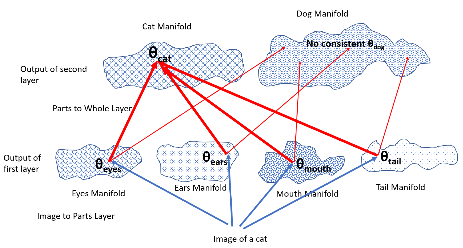
See Figure 15 for illustration of this approach which can be considered as a conceptual manifold formalization of ideas behind capsule networks [21]. The parameters for parts are mapped to the parameters of the cat by the neural network,

All the parts vote for a consistent pose of the cat and therefore there is redundancy between them. If there is significant redundancy and mutual information in terms of entropy, we will have

This keeps the dimensionality of the whole objects in check though it will increase gradually as their complexity increases. This efficient approach in keeping dimensionality low in every layer of the neural network can be considered as very effective compression of the scene and as combining generative approach with discriminative approach. The generative model ensures that pose parameters are semantically meaningful. Low dimensionality assures us that we are getting close to dimensionality of underlying image manifolds.

Even separate objects which have consistent poses statistically can all work together in agreeing on correct scene interpretation. For example, in a traffic scene for self-driving cars, different objects can consistently vote for the pose of the road.

Objects can be totally unrelated with no mutual information and in that case dimensions will just add. To have both house and cat, the embedded subspace dimensionality will be

which renders the joint scene of cat with background of house. Note that parameters will also include extra scene parameters, such as viewpoint and lighting, to generatively create a 2-D image from the 3-D world, which may be same for cat and house. So even for seemingly unrelated objects there may be some redundancy as they are part of the same scene.

For future improvements, we should be able to infer these generative parameters and mappings of points from one manifold to another manifold for complex scenes. This can be done using both explicit and implicit approaches.

1. (1)

   We train neurons for hierarchy of parts in which the training data has explicit ground truth for poses of parts and objects. Neurons have regression loss function for these pose parameters, along with discriminative loss and generative loss.

2. (2)

   Ground truth is simpler without detailed annotations of parts and relationships. We estimate potential number of parts and pose parameters and design the architecture of the network accordingly. We let the network learn these implicitly through a combination of discriminative loss and generative loss as is done in capsule networks, see [21].

Such networks will have following strengths.

1. (1)

   The need for getting training data for all poses and variations gets restricted to smallest parts which have low dimensionality and therefore it is practically feasible.

2. (2)

   Initial neuron layer needs to predict pose parameters of only fundamental parts from regions of raw images and therefore the number of parameters remain in check once again due to low dimensionality. For higher layers, neurons have to map points from one manifold to another and with ingenious work in future hopefully it will be practically feasible as we keep dimensionality in check at each layer.

3. (3)

   The neural network has generative component in form of pose parameters defined either explicitly or implicitly.

4. (4)

   The neural network is better implementation of parts-whole manifold learning hypothesis. Therefore, it learns semantically meaningful high-level abstractions rather than superficial and coarse geometries of manifolds.

Successful outcome of the above work should eliminate adversarial examples. If human vision does not suffer from adversarial examples, computer vision should not either.

References

- [1] Naveed Akhtar and Ajmal Mian, Threat of adversarial attacks on deep learning in computer vision: a survey, https://arxiv.org/abs/1801.00553v1 (2018).
- [2] Laurent Amsaleg, James Bailey, Dominique Barbe, Sarah Erfani, Michael E. Houle, Vinh Nguyen, and Milos Radovanovic, The vulnerability of learning to adversarial perturbation increases with ? intrinsic dimensionality, Proc. of IEEE WIFS (2017).
- [3] A. J. Bray and D. S. Dean, Statistics of critical points of gaussian fields on large-dimensional spaces, Physics Review Letter, 98, 150201 (2007).
- [4] Anna Choromanska, Mikael Henaff, Michael Mathieu, Gérard Ben Arous and Yann LeCun, The loss surfaces of multilayer networks, Proc. of 18th Intnl. Conf. on AI and Statistics, San Diego (2015), JMLR: W & CP, Volume 18, https://arxiv.org/abs/1412.0233 (2014).
- [5] David S. Dean and Satya N. Majumdar, Large deviations of extreme eigenvalues of random matrices, Phys.Rev.Lett. 97, 160201, https://doi.org/10.1103/PhysRevLett.97.160201 (2006).
- [6] Jean-Pierre Dedieu and Gregorio Malajovich, On the number of minima of a random polynomial, Journal of Complexity, Volume 24, Issue 2 (April), Pages 89-108, https://doi.org/10.1016/j.jco.2007.09.003 (2008).
- [7] Yann N. Dauphin, Razvan Pascanu, Caglar Gulcehre, Kyunghyun Cho, Surya Ganguli and Yoshua Bengio, Identifying and attacking the saddle point problem in high-dimensional non-convex optimization, https://arxiv.org/pdf/1406.2572.pdf (2014).
- [8] Herbert Federer, Geometric measure theory, Springer-Verlag (1969).
- [9] Charles Fefferman, Sanjoy Mitter and Hariharan Narayanan, Testing the manifold hypothesis, Journal of the American Mathematical Society, Volume 29, Number 4, October, Pages 983-1049, http://dx.doi.org/10.1090/jams/852 (2016).
- [10] Ian J. Goodfellow, Jonathon Shlens and Christian Szegedy, Explaining and harnessing adversarial examples, Proc. of ICLR 2015, https://arxiv.org/pdf/1412.6572.pdf (2015).
- [11] Matthias Hein and Maksym Andriushchenko, Formal Guarantees on the Robustness of a Classifier against Adversarial Manipulation, arxiv preprint arXiv:1705.08475 (2017).
- [12] Jason Jo and Yoshua Bengio, Measuring the tendency of CNNs to learn surface statistical regularities, arXiv preprint arXiv:1711.11561 (2017).
- [13] Alexey Kurakin, Ian J. Goodfellow and Samy Bengio, Adversarial examples in the physical world, Proc. of ICLR 2017, https://arxiv.org/pdf/1607.02533.pdf (2017).
- [14] Qianli Liao and Tomaso Poggio, Theory II: Landscape of the empirical risk in deep learning, https://arxiv.org/abs/1703.09833v2 (2017).
- [15] Xingjun Ma, Bo Li, Yisen Wang, Sarah M. Erfani, Sudanthi Wijewickrema, Michael E. Houle, Grant Schoenebeck, Dawn Song, and James Bailey, Characterizing adversarial subspaces using local intrinsic dimensionality, https://arxiv.org/abs/1801.02613v1 (2018).
- [16] Manifold learning theory and applications, CRC Press, Boca Raton, FL. Edited by Yunqian Ma and Yun Fu (2018).
- [17] Guido Montúfar, Razvan Pascanu, Kyunghyun Cho and Yoshua Bengio, On the number of linear regions of deep neural networks, Proc. of NIPS 2014, Pages 2924-2932 (2014).
- [18] A. Nguyen, J.Yosinski and J. Clune, Deep neural networks are easily fooled: High confidence predictions for unrecognizable images, Proc. of CVPR 2015, https://arxiv.org/pdf/1412.1897.pdf (2015).
- [19] Quynh Nguyen and Matthias Hein, The loss surface of deep and wide neural networks, https://arxiv.org/abs/1704.08045 (2017).
- [20] Tomaso Poggio, Kenji Kawaguchi, Qianli Liao, Brando Miranda, Lorenzo Rosasco, Xavier Boix, Jack Hidary and Hrushikesh Mhaskar, Theory of deep learning III: explaining the non-overfitting puzzle, https://arxiv.org/abs/1801.00173v1 (2017).
- [21] Sara Sabour, Nicholas Frosst and Geoffrey E Hinton, Dynamic routing between capsules, https://arxiv.org/abs/1710.09829 (2017).
- [22] Levent Sagun, Leon Bottou and Yann LeCun, Eigenvalues and the Hessian in deep learning: Singularity and beyond, https://openreview.net/pdf?id=B186cP9gx (2017).
- [23] A. van der Schaafa and J.H. van Haterena, Modelling the power spectra of natural images: Statistics and information, Vision Research, Volume 36, Issue 17 (September), Pages 2759-2770 (1996).
- [24] A. Srivastava, A. Lee, E. Simoncelli and S.-C. Zhu, On advances in statistical modeling of natural images, Journal of Mathematical Imaging and Vision 18: 17. https://doi.org/10.1023/A:1021889010444 (2003).
- [25] M. Stone, The generalized Weierstrass approximation theorem, Mathematics Magazine 21 (21), 167-184 and 21 (5), 237-254 (1948).
- [26] Gilbert Strang and Truong Nguyen, Wavelets and filter banks, Wellesley-Cambridge Press, 2nd edition (1996).
- [27] Christian Szegedy, Wojciech Zaremba, Ilya Sutskever, Joan Bruna, Dumitru Erhan, Ian J. Goodfellow and Rob Fergus, Intriguing properties of neural networks, Proc. of ICLR 2014, http: //arxiv.org/abs/1312.6199 (2014).
- [28] Thomas Tanay and Lewis Griffin, A boundary tilting persepective on the phenomenon of adversarial examples, https://arxiv.org/abs/1608.07690 (2016).
- [29] M. B. Wakin, D. L. Donoho, H. Choi, and R. G. Baraniuk, The multiscale structure of non-differentiable image manifolds, In SPIE Optics and Photonics, volume 5914, pages 413 - 429 (2005).