Dynamic Channel Bonding in Spatially Distributed High-Density WLANs
Abstract
In this paper, we discuss the effects on throughput and fairness of dynamic channel bonding (DCB) in spatially distributed high-density wireless local area networks (WLANs). First, we present an analytical framework based on continuous-time Markov networks (CTMNs) for depicting the behavior of different DCB policies in spatially distributed scenarios, where nodes are not required to be within the carrier sense range of each other. Then, we assess the performance of DCB in high-density IEEE 802.11ac/ax WLANs by means of simulations. We show that there may be critical interrelations among nodes in the spatial domain – even if they are located outside the carrier sense range of each other – in a chain reaction manner. Results also reveal that, while always selecting the widest available channel normally maximizes the individual long-term throughput, it often generates unfair situations where other WLANs starve. Moreover, we show that there are scenarios where DCB with stochastic channel width selection improves the latter approach both in terms of individual throughput and fairness. It follows that there is not a unique optimal DCB policy for every case. Instead, smarter bandwidth adaptation is required in the challenging scenarios of next-generation WLANs.
1 Introduction
Wireless local area networks (WLANs), with IEEE 802.11 as the most widely used standard, are a cost-efficient solution for wireless Internet access that can satisfy most of the current communication requirements in domestic, public, and business scenarios. However, the scarcity of the frequency spectrum in the industrial, scientific and medical (ISM) radio bands, the increasing throughput demands given by new hungry-bandwidth applications, and the heterogeneity of current wireless network deployments give rise to substantial complexity. Such issues gain importance in dense WLAN deployments, leading to multiple partially overlapping scenarios and coexistence problems.
In this regard, two main approaches to optimizing the scarce resources of the frequency spectrum are being deeply studied in the context of WLANs: channel allocation (CA) and channel bonding (CB). While CA refers to the action of allocating the potential transmission channels (i.e., both the primary and secondary channels) for a WLAN or group of WLANs, CB is the technique whereby nodes are allowed to use a contiguous set of idle channels for transmitting in larger bandwidths, thus potentially achieving a higher throughput.
This paper focuses on CB, which was first introduced in the IEEE 802.11n (11n) amendment by allowing two 20 MHz basic channels to be aggregated into a 40 MHz channel. Newer amendments like IEEE 802.11ac (11ac) extend the number of basic channels that can be aggregated up to 160 MHz channel widths. It is expected that IEEE 802.11ax (11ax) will boost the use of wider channels [1]. Nonetheless, due to the fact that using wider channels increases the contention and interference among nodes, undesirable lower performances may be experienced when applying static channel bonding (SCB), especially in high-density WLAN scenarios. To mitigate such a negative effect, dynamic channel bonding (DCB) policies are used to select the bandwidth in a more flexible way based on the instantaneous spectrum occupancy. A well-known example of DCB policy is always-max (AM)11 1 Some papers in the literature indistinctively use the terms DCB and AM. In this paper, we notate AM as a special case of DCB. [2, 3], where transmitters select the widest channel found idle when the backoff counter terminates. To the best of our knowledge, the works in the literature assessing the performance of DCB only study the SCB and AM policies, while they also assume fully overlapping scenarios where all the WLANs are within the carrier sense range of the others [4, 5, 2, 6]. Therefore, there is an important lack of insights on the performance of CB in more realistic WLAN scenarios, where such a condition usually does not hold.
With this work, we aim to extend the state of the art by providing new insights on the performance of DCB under saturation regimes in WLAN scenarios that are not required to be fully overlapping; where the effect of carrier sense and communication ranges play a crucial role due to spatial distribution interdependencies. Namely, the operation of a node has a direct impact on the nodes inside its carrier sense range, which in turn may affect nodes located outside such range in complex and hard to prevent ways. Besides, we assess different DCB policies, including a stochastic approach that selects the channel width randomly.
In order to evaluate different DCB policies, we first introduce the Spatial-Flexible Continuous Time Markov Network (SFCTMN), an analytical framework based on continuous-time Markov networks (CTMNs). This framework is useful for describing the different phenomena that occur in WLAN deployments when considering DCB in spatially distributed scenarios. In this regard, we analytically depict such complex phenomena by means of illustration through several toy scenarios. Finally, we evaluate the performance of the proposed policies in large high-density 11ax WLAN scenarios by means of simulations using Komondor, a particular release (v1.0.1) of the Komondor [7] wireless networks simulator.22 2 All of the source code of SFCTMN and Komondor is open, encouraging sharing of algorithms between contributors and providing the ability for people to improve on the work of others under the GNU General Public License v3.0. The repositories can be found at https://github.com/sergiobarra/SFCTMN and https://github.com/wn-upf/Komondor, respectively. We find that, while AM is normally the best DCB policy for maximizing the individual long-term throughput of a WLAN, it may generate unfair situations where some other WLANs starve. In fact, there are cases where less aggressive policies like stochastic channel width selection improve AM both in terms of individual throughput and fairness. This leads to the need of boosting wider channels through medium adaptation policies. The contributions of this paper are as follows:
- 1.
Novel insights on the effects of DCB in high-density scenarios. We depict the complex interactions given in spatially distributed deployments – i.e., considering path loss, signal-to-interference-plus-noise ratio (SINR) and clear channel assessment (CCA) thresholds, co-channel and adjacent channel interference, etc. – and discuss the influence that nodes have among them.
- 2.
Generalization of DCB policies including only-primary (i.e., selecting just the primary channel for transmitting), SCB, AM, and probabilistic uniform (PU) (i.e., selecting the channel width stochastically).
- 3.
Algorithm for modeling WLAN scenarios with CTMNs that extends the one presented in [6]. Such an extension allows us capturing non-fully overlapping scenarios, taking into consideration spatial distribution implications. Moreover, this algorithm allows us to model any combination of DCB policies in a network.
- 4.
Performance evaluation of the presented DCB policies in high-density WLAN scenarios by means of simulations. The selected physical (PHY) and medium access control (MAC) parameters are representative of single user (SU) transmissions in 11ax WLANs.
2 Related work
Several works in the literature assess the performance of CB by means of analytical models, simulations or testbeds. Authors in [8, 9] experimentally analyze SCB in IEEE 802.11n WLANs and show that the reduction of Watt/Hertz when transmitting in larger channel widths causes lower SINR at the receivers. This lessens the coverage area consequently and increases the probability of packet losses due to the accentuated vulnerability to interference. Nonetheless, they also show that DCB can provide significant throughput gains when such issues are palliated by properly adjusting the transmission power and data rates.
The advantages and drawbacks of CB are accentuated with the 11ac and 11ax amendments since larger channel widths are allowed (up to 160 MHz). Nevertheless, it is important to emphasize that in the dense and short-range WLAN scenarios expected in the coming years [1], the issues concerning low SINR values may be palliated. The main reason lies in the shorter distances between transceiver and receiver, and the usage of techniques like spatial diversity multiple-input multiple-output (MIMO)[10]. An empirical study on CB in 11ac is followed in [11], where authors show that throughput increases by bonding channels. By means of simulations, authors in [12, 3] assess the performance of DCB in 11ac WLANs, resulting in significant throughput gains. Still, they also corroborate that these gains are severely compromised by the activity of overlapping wireless networks.
There are other works in the literature that follow an analytical approach for assessing the performance of CB. For instance, authors in [4] analytically model and evaluate the performance of CB in short-range 11ac WLANs, proving significant performance boost in presence of low to moderate external interference. In [2], authors show that CB can provide significant performance gains even in high-density scenarios, though it may also cause unfairness. Non-saturation regimes are considered in [13, 14], where authors propose an analytical model for the throughput performance of CB in 11ac/11ax WLANs under both saturated and non-saturated traffic loads. An analytical framework to study the performance of opportunistic CB where 11ac users coexist with legacy users is presented in [15]. Recently, an analytical model based on renewal theory showed that 11ac/11ax DCB can improve throughput even in the presence of legacy users [16]. Literature on CTMN models for DCB WLANs is further discussed in Section 4.
As for particular CB solutions or algorithms, an intelligent scheme for jointly adopting the rate and bandwidth in MIMO 11n WLANs is presented in [10]. Testbed experiments show that such scheme (ARAMIS) accurately adapts to a wide variety of channel conditions with negligible overhead and achieving important performance gains. A DCB protocol with collision detection is presented in [17], in which a node gradually increases the transmission bandwidth whenever new narrow channels are found available. A stochastic spectrum distribution framework accounting for WLANs demand uncertainty is presented in [18], showing better performance compared to the naive allocation approach. Authors in [19] show that the maximal throughput performance can be achieved with DCB under the CA scheme with the least overlapped channels among WLANs. A dynamic bandwidth selection protocol for 11ac WLANs is proposed in [20] to prevent the carrier sensing decreasing and outside warning range problems. In [16] authors propose a heuristic primary channel selection for maximizing the throughput of multi-channel users. Finally, [21] proposes a prototype implementation for commercial 11ac devices showing up to 1.85x higher throughput when canceling time-domain interference.
We believe that this is the first work providing insights into the performance of DCB in spatially distributed scenarios, where the effect of partially overlapping nodes plays a crucial role due to the spatial interdependencies. We also provide an algorithm for generating the CTMNs to model such kind of scenarios. Besides, we assess the performance of different DCB policies, including a novel stochastic approach, and show that always selecting the widest available channel may be sub-optimal in some scenarios.
3 System model under consideration
In this section, we first depict the notation regarding channelization that is used throughout this article. We also define the DCB policies that are studied and provide a general description of the carrier sense multiple access with collision avoidance (CSMA/CA) operation in IEEE 802.11 WLANs. Finally, we expose the main assumptions considered in the presented scenarios.
3.1 Channelization
Let us discuss the example shown in Figure 1 for introducing the channel access terminology and facilitating further explanation. In this example, the system channel counts with basic channels and WLAN X is allocated with the channel and primary channel . Note that in this particular example the AP of WLAN X does not select the entire allocated channel, but a smaller one, i.e., . Two reasons may be the cause: i) basic channels 1 and/or 2 are detected busy at the end of the backoff, or ii) the DCB policy determines not to pick them. More formally, the definitions of the channelization terms used throughout the paper are as follows:
- •
Basic channel : the frequency spectrum is split into basic channels of width MHz.
- •
Primary channel : a basic channel with different roles depending on the node state. All the nodes belonging to the same WLAN must share the same primary channel . Essentially, this channel is used to i) sense the medium for decrementing the backoff when the primary channel’s frequency band is found free, and ii) listening to control and data packets.
- •
Channel : a channel consists of a contiguous set of basic channels. The width (or bandwidth) of a channel is .
- •
Channelization scheme : the set of channels that can be used for transmitting is determined by the channel access specification and the system channel (), whose bandwidth is given by . Namely, all the nodes in the system must transmit in some channel included in . A simplified version of the channelization considered in the 11ac and 11ax standards is shown in Figure 2, .
- •
WLAN’s allocated channel : nodes in a WLAN must transmit in a channel contained in . Different WLANs may be allocated with different primary channels and different available channel widths.
- •
Transmission channel : a node belonging to a WLAN has to transmit in a channel , which will be given by i) the set of basic channels in found idle by node at the end of the backoff (),33 3 Note that, in order to include secondary channels for transmitting, a WLAN must listen them free during at least a point coordination function interframe space (PIFS) period before the backoff counter terminates as shown in Figure 3. While such PIFS condition is not considered in the SFCTMN framework for the sake of analysis simplicity, the Komondor simulator does. and ii) the implemented DCB policy.


3.2 CSMA/CA operation in IEEE 802.11 WLANs
According to the CSMA/CA operation, when a node belonging to a WLAN has a packet ready for transmission, it measures the power sensed in the frequency band of . Once the primary channel has been detected free, i.e., the power sensed by at is smaller than its CCA threshold, the node starts the backoff procedure by selecting a random initial value of time slots of duration . The contention window is defined as , where is the backoff stage with maximum value , and is the minimum contention window. When a packet transmission fails, is increased by one unit, and reset to 0 when the packet is acknowledged.
After computing BO, the node starts decreasing the backoff counter while sensing the primary channel. Whenever the power sensed by at is higher than its CCA, the backoff is paused and set to the nearest higher time slot until is detected free again, at which point the countdown is resumed. When the backoff timer reaches zero, the node selects the transmission channel based on the set of idle basic channels and on the DCB policy. The selected transmission channel is then used throughout the whole packet exchanges involved in a data packet transmission between the transceiver and receiver. Namely, request to send (RTS) – used for notifying the selected transmission channel – clear to send (CTS), and acknowledgment (ACK) packets are also transmitted in . Likewise, any other node that receives an RTS in its primary channel with enough power to be decoded will enter in network allocation vector (NAV) state, which is used for deferring channel access and avoiding packet collisions (especially those caused by hidden node situations).
3.3 DCB policies
The DCB policy determines the transmission channel a node must pick from the set of available ones. When the backoff terminates, any node belonging to a WLAN operates according to the DCB policy as follows:
- •
Only-primary (OP) or single-channel: pick just the primary channel for transmitting if it is found idle.
- •
Static channel bonding (SCB): exclusively pick the full channel allocated in its WLAN when found free. Namely, nodes operating under SCB cannot transmit in channels different than .
- •
Always-max (AM): pick the widest possible channel found free in for transmitting.
- •
Probabilistic uniform (PU): pick with same probability any of the possible channels found free inside the allocated channel .
For the sake of illustration, let us consider the example shown in Figure 3, which shows the evolution of a node implementing different DCB policies. In this example, a node is allowed to transmit in the set of basic channels , where is the primary channel. While OP picks just the primary channel, the rest of policies try to bond channels in different ways. In this regard, SCB is highly inefficient in scenarios with partial interference. In fact, no packets can be transmitted with SCB in this example since the basic channel is busy during the PIFS durations previous to the backoff terminations. However, more flexible approaches like AM and PU are able to transmit more than one frame in the same period of time. On the one hand, AM adapts in an aggressive way to the channel state. Specifically, it is able to transmit in 40 and 80 MHz channels at the end of the first and second backoff, respectively. On the other hand, the stochastic nature of PU makes it more conservative than AM. In the example, the node could transmit in 1 or 2 basic channels with the same probability (1/2) at the end of the first backoff. Likewise, after the second backoff, a channel composed of 1, 2 or 4 basic channels could be selected with probability (1/3).
3.4 Main assumptions
In this paper, we present results gathered via the SFCTMN framework based on CTMNs, and also via simulations through the Komondor wireless network simulator. While in the latter case we are able to introduce more realistic implementations of the 11ax amendment, in the analytical model we use relaxed assumptions for facilitating subsequent analysis. This subsection depicts the general assumptions considered in both cases.
- 1.
Channel model: signal propagation is isotropic. Also, the propagation delay between any pair of nodes is considered negligible because of the small carrier sense in the above 1GHz ISM bands where WLANs operate. Besides, the transmission power is divided uniformly among the basic channels in the selected transmission channel. We also consider an adjacent channel interference model that replicates of the power transmitted per Hertz into the two basic channels that are contiguous to the actual transmission channel.
- 2.
Packet errors: a packet is lost if i) the power of interest received at the receiver is less than its CCA, ii) the SINR () perceived at the receiver does not accomplish the capture effect (CE), i.e., CE, or iii) the receiver was already receiving a packet. In the latter case, the decoding of the first packet is ruptured only if the CE is no longer accomplished because of the interfering transmission. We assume an infinite maximum number of retransmissions per packet, whose effect is negligible in most of the cases because of the small probability of retransmitting a data packet more than few times [22].
- 3.
Modulation and coding scheme (MCS): the MCS index used by each WLAN is the highest possible according to the SINR perceived by the receiver, and it is kept constant throughout all the simulation. We assume that the MCS selection is designed to keep the packet error rate constant and equal to given that static deployments are considered.44 4 In 802.11 devices, given a minimum receiver sensitivity and SINR table, a maximum decoding packet error rate of 10% is usually tried to be guaranteed when selecting the MCS index. Note that the value is only considered if none of the three possible causes of packet error explained in the item above are given.
- 4.
Traffic: downlink traffic is considered. In addition, we assume a full-buffer mode where APs always have backlogged data pending for transmission.
4 The CTMN model for WLANs
The analysis of CSMA/CA networks through CTMN models was firstly introduced in [23]. Such models were later applied to IEEE 802.11 networks in [24, 6, 2, 13, 4, 19, 25, 14], among others. Experimental results in [26, 27] demonstrate that CTMN models, while idealized, provide remarkably accurate throughput estimates for actual IEEE 802.11 systems. A comprehensible example-based tutorial of CTMN models applied to different wireless networking scenarios can be found in [28]. Nevertheless, to the best of our knowledge, works that model DCB through CTMNs study just the SCB and AM policies, while assuming fully overlapping scenarios. Therefore, there is an important lack of insights on more general deployments, where such conditions usually do not hold and interdependencies among nodes may have a critical impact on their performance. For instance, an optimal channel allocation algorithm to achieve maximal throughput with DCB was recently presented in [29]. However, this work does not consider the implications of either spatial distribution nor CE.
In this section, we depict our extended version of the algorithm introduced in [6] for generating the CTMNs corresponding to spatially distributed WLAN scenarios, which is implemented in the SFCTMN framework. With this extension, as the condition of having fully overlapping networks is no longer required for constructing the corresponding CTMNs, more factual observations can be made.
4.1 Implications
Modeling WLAN scenarios with CTMNs requires the backoff and transmission times to be exponentially distributed. It follows that, because of the negligible propagation delay, the probability of packet collisions between two or more nodes within the carrier sense range of the others is zero. The reason is that two WLANs will never end their backoff at the same time, and therefore they will never start a transmission at the same time either. Besides, in overlapping single-channel CSMA/CA networks, it is shown that the state probabilities are insensitive to the backoff and transmission time distributions [27, 30]. However, even though authors in [6] prove that the insensitivity property does not hold for DCB networks, the sensitivity to the backoff and transmission time distributions is very small. Therefore, the analytical results obtained using the exponential assumption offer a good approximation for deterministic distributions of the backoff, data rate, and packet length.
4.2 Constructing the CTMN
In order to depict how CTMNs are generated, let us consider the toy scenario (Scenario I) shown in Figure 4, which is composed of two fully overlapping WLANs implementing AM.55 5 Scenario I is selected for conveniently depicting the algorithm. CTMNs corresponding to non-fully overlapping scenarios (e.g., Scenario III in Section 5) can be also generated with the very same algorithm. The channel allocation employed in such a scenario can be defined as with , and with . That is, there are four basic channels in the system, and the set of valid transmission channels according to the 11ax channel access scheme is (see Figure 2). Due to the fact that both WLANs are inside the carrier sense range of each other, their APs could transmit simultaneously at any time only if their transmission channels do not overlap, i.e., . Notice that slotted backoff collisions cannot occur because their counters decrease continuously in time, and therefore two transmissions can be neither started nor finished at the very same time.
4.2.1 States
A state in the CTMN is defined by the set of WLANs active and the basic channels on which they are transmitting. Essentially, we say that a WLAN is active if it is transmitting in some channel, and inactive otherwise. We define two types of state spaces: the global state space () and the feasible state space ().

- •
Global state space: a global state is a state that accomplishes two conditions: i) the channels in which the active WLANs are transmitting comply with the channelization scheme , and ii) all active WLANs transmit inside their allocated channels. That is, only depends on the particular channelization scheme in use and on the channel allocation of the WLANs in the system. In this paper, we assume that every transmission should be made in channels inside that are composed of contiguous basic channels, for some integer , and that their rightmost basic channels fall on multiples of , as stated in the 11ac and 11ax amendments.
- •
Feasible state space: a feasible state exists only if each of the active WLANs in such state started their transmissions by accomplishing the CCA requirement derived from the assigned DCB policy. Namely, given a global state space, depends only on the spatial distribution and on the DCB policies assigned to each WLAN.
The CTMN corresponding to the toy Scenario I is shown in Figure 5. Regarding the notation, we represent the states by the most left and most right basic channels used in the transmission channels of each of their active WLANs. For instance, state refers to the state where A and B are transmitting in channels and , respectively. Concerning the state spaces, states , , , , , , are not reachable (i.e., they are global but not feasible) for two different reasons. First, states and are not feasible because of the overlapping channels involved. Secondly, the rest of unfeasible states are so due to the fact that AM is applied, thus at any time that WLAN A(B) finishes its backoff and B(A) is not active, A(B) picks the widest available channel, i.e., or , respectively. Likewise, any time A(B) finishes its backoff and B(A) is active, A(B) picks again the widest available channel, which in this case would be for A and for B if A is not transmitting in its full allocated channel, respectively. Some states such as are reachable only via backward transitions. In this case, when A finishes its backoff and B is transmitting in (i.e., ), A picks just because the power sensed in channels 3 and 4 exceeds the CCA as a consequence of B’s transmission. That is, is only reachable through a backward transition from , given when B finishes its transmission in state .
4.2.2 CTMN algorithm: finding states and transitions
The first step for constructing the CTMN is to identify the global state space , which is simply composed by all the possible combinations given by the system channelization scheme and the channel allocations of the WLANs. The feasible states in are later identified by exploring the states in . Algorithm 1 shows the pseudocode for identifying both and the transitions among such states, which are represented by the transition rate matrix .66 6 Notice that we use to say that a WLAN X transmits in a range of contiguous basic channels when the CTMN is in state . With slight abuse of notation, represents the state where all WLANs that were active in remain active except for X, which becomes inactive after finishing its packet transmission. Similarly, , represents the state where all the active WLANs in remain active and X is transmitting in the range of basic channels .
Essentially, while there are discovered states in that have not been explored yet, for any state not explored, and for each WLAN X in the system, we determine if X is active or not. If X is active, we then set possible backward transitions to already known and not known states. To do so, it is required to fully explore looking for states where: i) other active WLANs in the state remain transmitting in the same transmission channel, and ii) WLAN X is not active.
On the other hand, if WLAN X is inactive in state , we try to find forward transitions to other states. To that aim, the algorithm fully explores looking for states where i) other active WLANs in the state remain transmitting in the same transmission channel, and ii) X is active in the new state as a result of applying the implemented DCB policy () as shown in line 1. It is important to remark that in order to apply such policy, the set of idle basic channels in state , i.e., , must be identified according to the power sensed in each of the basic channels allocated to X, i.e., , and on its CCA level. Thereafter, the transmission channel is selected through the function, which applies .
Each transition between two states and has a corresponding transition rate . For forward transitions, the packet transmission attempt rate (or simply backoff rate) has an average duration , where is the expected backoff duration in time slots, determined by the minimum contention window, i.e., . Furthermore, for backward transitions, the departure rate () depends on the duration of a successful transmission, i.e., , which in turn depends on both the data rate () given by the selected MCS and transmission channel width, and on the packet length . In the algorithm, we simply consider that the data rate of a WLAN X depends on the state of the system, which collects such information, i.e., .
Depending on the DCB policy, different feasible forward transitions may exist from the very same state, which are represented by the set . As shown in line 1, every feasible forward transition rate is weighted by a transition probability vector () whose elements determine the probability of transiting to each of the possible global states in . Namely, with a slight abuse of mathematical notation, the probability to transit to any given feasible state is . As a consequence, must follow the normalization condition .
For the sake of illustration, in the CTMNs of Figures 5, 7 and 9, states are numbered according to the order in which they are discovered. Transitions between states are also shown below the edges. Note that with SFCTMN, since non-fully overlapping networks are allowed, transitions to states where one or more WLANs may suffer from packet losses due to interference are also reachable (see Section 5).
4.3 Performance metrics
Since there are a limited number of possible channels to transmit in, the constructed CTMN will always be finite. Furthermore, it will be irreducible due to the fact that backward transitions between neighboring states are always feasible. Therefore, a steady-state solution to the CTMN always exists. However, due to the possible existence of one-way transitions between states, the CTMN is not always time-reversible and the local balance may not hold [31]. Accordingly, it prevents to find simple product-from solutions to compute the equilibrium distribution of the CTMNs. The equilibrium distribution vector represents the fraction of time the system spends in each feasible state. Hence, we define as the probability of finding the system at state . In order to obtain we can use the transition rate matrix given the system of equations .
As an example, for Scenario I, considering that its elements are sorted by the discovery order of the states, . Besides, the corresponding transition rate matrix is
where , and , are the packet generation and departure rates in state of WLANs A and B, respectively. The diagonal elements represented by ‘*’ in the matrix should be replaced by the negative sum of the rest of items of their row, e.g., , but for the sake of illustration we do not include them in the matrix. Once is computed, estimating the average throughput experienced by each WLAN is straightforward. Specifically, the average throughput of a WLAN is
where is the expected data packet length, is the SINR perceived by the STA in WLAN in state , CE is the capture effect, and is the constant packet error probability. The system aggregate throughput is therefore the sum of the throughputs of all the WLANs, i.e., . Besides, in order to evaluate the fairness of a given scenario, we can use and/or , for proportional fairness and the Jain’s Fairness Index, respectively.
4.4 Captured phenomena
Even though most of the well-known wireless phenomena are captured by SFCTMN, there are some important features that cannot be implemented due to its mathematical modeling nature. Essentially, the main limitations are the inability to capture backoff collisions and the constraints in terms of execution time for medium size networks. Besides, only the overhead of the RTS/CTS packets are considered in SFCTMN, i.e., the time of a successful transmission takes also the transmission time of such packets into account. However, the main purpose of the RTS/CTS mechanism of avoiding hidden nodes is not captured by the generated CTMNs since no packets are actually transmitted. That is, only average performance is captured through states modeled without differentiating from the type of packet being transmitted.
To cope with the abovementioned limitations, we make use of a simulator in Section 6. Basically, when we lose the benefits of analytically modeling the networks, with Komondor we are allowed to simulate large networks and get more realistic insights. A comparison of the features implemented in each tool is shown in Table 1.
5 Interactions in frequency and space
In this section, we draw some relevant conclusions about applying different DCB policies in CSMA/CA WLANs by analyzing four representative toy scenarios with different channel allocations and spatial distributions. To that aim, we use the SFCTMN analytical framework and validate the gathered results by means of the Komondor wireless network simulator.77 7 For the sake of saving space, the evaluation setups and corresponding results of the scenarios considered through the paper are detailed in https://github.com/sergiobarra/data_repos/tree/master/barrachina2018performance
In summary, the main outcomes derived from the analytical analyses performed below in this section are: i) the feasible system states depend on the DCB policies followed by each of the WLANs, ii) maximizing the instantaneous throughput may not be the optimal strategy to maximize the long-term throughput, iii) in non-fully overlapping scenarios, cumulative interference and flow starvation may appear and cause poor performance to some WLANs, iv) there is not a unique optimal DCB policy. Note that, otherwise stated, in this paper the optimal DCB policy for WLAN is the one that maximizes its throughput, i.e., .
5.1 Feasible states dependence on the DCB policy
In Table 2 we show the effect of applying different DCB policies on the average throughput experienced by WLANs A and B ( and , respectively), and by the whole network () in scenarios I and II (presented in Figures 4 and 6, respectively). Let us first consider Scenario I. As explained in Section 4 and shown in Figure 5, the CTMN reaches 5 feasible states when WLANs implement AM. Instead, due to the fact that both WLANs overlap in channels 3 and 4 when transmitting in their whole allocated channels – i.e., and , respectively – the SCB policy reaches just three feasible states. Such states correspond to those with a single WLAN transmitting, i.e., , , . In the case of OP, both WLANs are forced to pick just their primary channel for transmitting and, therefore, . Notice that state is feasible because A and B have different primary channels and do not overlap when transmitting in them.
| Tool | SFCTMN | Komondor |
|---|---|---|
| Type | Analytical model | Simulator |
| DCB policies | ✓ | ✓ |
| Hidden & exposed nodes | ✓ | ✓ |
| RTS/CTS | ✗(a) | ✓ |
| Flow-in-the-middle | ✓ | ✓ |
| Information asymmetry | ✓ | ✓ |
| Backoff collision | ✗ | ✓ |
| Scalable(b) | ✗ | ✓ |
- •
RTS/CTS overhead considered in throughput measurements.
- •
Assumable execution time for up to 300 nodes.
| Policy | Scenario I | Scenario II | ||||||
|---|---|---|---|---|---|---|---|---|
| OP | 4 | 109.36 | 109.36 | 109.36 | 4 | 109.36 | 109.36 | 109.36 |
| (109.36) | (109.36) | (109.36) | (109.36) | (109.36) | (109.36) | |||
| SCB | 3 | 132.75 | 132.75 | 132.75 | 3 | 102.65 | 102.65 | 102.65 |
| (123.21) | (137.09) | (130.15) | (102.24) | (102.24) | (102.24) | |||
| AM | 5 | 206.68 | 199.67 | 203.17 | 3 | 102.65 | 102.65 | 102.65 |
| (204.70) | (201.91) | (203.31) | (102.24) | (102.24) | (102.24) | |||
| PU | 10 | 142.70 | 142.00 | 142.35 | 6 | 109.30 | 109.30 | 109.30 |
| (142.69) | (142.01) | (142.35) | (109.29) | (109.27) | (109.28) | |||
The last policy studied is PU, which is characterized by providing further exploration of the global state space . It usually allows expanding the feasible state space accordingly because more transitions are permitted. In Scenario I, whenever the CTMN is in state and the backoff of A or B expires, the WLANs pick each of the possible available channels with the same probability. Namely, the CTMN will transit to , or with probability 1/3 when A’s backoff counter terminates, and to or with probability 1/2 whenever B’s backoff counter terminates.
Likewise, if the system is in state and A terminates its backoff counter, the CTMN will transit to the feasible states or with probability 1/2. Similarly, whenever the system is in state or , and B finishes its backoff, B will pick the transmission channels or with same probability 1/2 making the CTMN to transit to the corresponding state where both WLANs transmit concurrently. These probabilities are called transition probabilities and are represented by the vector . For instance, in the latter case, the probability to transit from to when B terminates its backoff is .
5.2 Instantaneous vs. long-term throughput
Intuitively, one could think that, as it occurs in Scenario I, always picking the widest channel found free by means of AM, i.e., maximizing the throughput of the immediate packet transmission (or instantaneous throughput), may be the best strategy for maximizing the long-term throughput as well. However, the Scenario II depicted in Figure 6 is a counterexample that illustrates such lack of applicable intuition. It consists of two overlapping WLANs as in Scenario I, but with different channel allocation: with and , respectively. The CTMNs that are generated according to the different DCB policies – generalized to any value the corresponding transition probabilities may have – are shown in Figure 7.

Regarding the transition probabilities, Table 3 shows the vectors that are given for each of the studied DCB policies in Scenario II. Firstly, with OP, due to the fact that WLANs are only allowed to transmit in their primary channel, the CTMN can only transit from state to states or , i.e., . Similarly, with SCB, WLANs can only transmit in their complete allocated channel, thus, when being in state the CTMN transits only to or , i.e., . Notice that AM generates the same transition probabilities (and respective average throughput) than SCB because whenever the WLANs have the possibility to transmit – which only happens when the CTMN is in state – both A and B pick the widest channel available, i.e., . Finally, PU picks uniformly at random any of the possible transitions that A and B provoke when terminating their backoff in state , i.e., and , respectively.
Note that state , when both WLANs are transmitting at the same time, is reachable from states and for both OP and PU. In such states, when either A or B terminates its backoff and the other is still transmitting in its primary channel, only a transition to state is possible, i.e., .
| OP | 4 | 1.0 | 0.0 | 1.0 | 0.0 |
| SCB | 3 | 0.0 | 1.0 | 0.0 | 1.0 |
| AM | 3 | 0.0 | 1.0 | 0.0 | 1.0 |
| PU | 6 | 0.5 | 0.5 | 0.5 | 0.5 |


Interestingly, as shown in Table 2, applying OP in Scenario II, i.e., being conservative and unselfish, is the best policy to increase both the individual average throughput of A and B (, , respectively) and the system’s aggregated one (). Instead, being aggressive and selfish, i.e., applying SCB or AM, provides the worst results both in terms of individual and system’s aggregate throughput. In addition, PU provides similar results than OP in average because most of the times that A and B terminate their backoff counter, they can only transmit in their primary channel since the secondary channel is most likely occupied by the other WLAN. In fact, state is the dominant state for both OP and PU. Specifically, the probability of finding the CTMN in state , i.e., , is 0.9802 for OP and 0.9702 for PU, respectively. Therefore, the slight differences on throughput experienced with OP and PU are given because of the possible transition from to the states and in PU, where WLANs entirely occupy the allocated channel, thus preventing the other for decreasing its backoff.
Despite being a very simple scenario, we have shown that it is not straightforward to determine the optimal DCB policy that the AP in each WLAN must follow. Evidently, in a non-overlapping scenario, AM would be the optimal policy for both WLANs because of the non-existence of inter-WLAN contention. However, this is not a typical case in dense scenarios and, consequently, AM may not be adopted as de facto DCB policy, even though it provides more flexibility than SCB. This simple toy scenario also serves to prove that some intelligence should be implemented in the APs in order to harness the information gathered from the environment.
Concerning the throughput differences in the values obtained by SFCTMN and Komondor,88 8 In Komondor the throughput is simply computed as the number of useful bits (corresponding to data packets) that are successfully transmitted divided by the observation time of the simulation. we note that the main disparities correspond to the AM and SCB policies. It is important to remark that while SFCTMN considers neither backoff collisions nor NAV periods, Komondor actually does so in a more realistic way. Therefore, in Komondor, whenever there is a slotted backoff collision, the RTS packets can be decoded by the STAs in both WLANs if the CE is accomplished. That is why the average throughput is consequently increased.
Regarding the NAV periods, an interesting phenomenon occurs in Scenario I when implementing SCB, AM or PU. While the RTS packets sent by B cannot be decoded by A because its primary channel is always outside the possible transmission channels of B (i.e., or ), the opposite occurs when A transmits them. Due to the fact that the RTS is duplicated in each of the basic channels used for transmitting, whenever A transmits in its whole allocated channel, B is able to decode the RTS (i.e., ) and enters in NAV consequently.
5.3 Cumulative interference and flow starvation
When considering non-fully overlapping scenarios, i.e., where some of the WLANs are not inside the carrier sense range of the others, complex and hard to prevent phenomena may occur. As an illustrative example, let us consider the case shown in Figure 8(a), where 3 WLANs sharing a single channel (i.e., ) are deployed composing a line network. As the carrier sense range is fixed and is the same for each AP, by locating the APs at different distances we obtain different topologies that are worth to be analyzed. We name these topologies from T1 to T4 depending on the distance between consecutive APs, which increases according to the topology index. Notice that all the DCB policies discussed in this work behave exactly the same way in single-channel scenarios. Therefore, in this subsection, we do not make distinctions among them.
The average throughput experienced by each WLAN in each of the regions is shown in Figure 8(b). Regarding topology T1, when APs are close enough to be inside the carrier sense range of each other in a fully overlapping manner, the medium access is shared fairly because of the CSMA/CA mechanism. For that reason, the throughput is decreased to approximately 1/3 with respect to topology T4. Specifically, the system spends almost the same amount of time in the states where just one WLAN is transmitting, i.e., . The neighbor overlapping case in topology T2 is a clear case of flow-in-the-middle (FIM) starvation. Note that A and C can transmit at the same time whenever B is not active, but B can only do so when neither A nor C are active. Namely, B has very few transmission opportunities because A and C are transmitting almost permanently and B must continuously pause its backoff consequently.
An interesting and hard to prevent phenomenon occurs in the potential central node overlapping case at topology T3. Figure 9 shows the corresponding CTMN. In this case, the cumulated interference perceived by B from both A and C, prevents the former to decrease its backoff, thus generating a new FIM-like scenario such as in topology T2. However, in this case, B is able to decrement the backoff any time A or C are not transmitting. This leads to two possible outcomes regarding packet collisions. On the one hand, if the capture effect condition is accomplished by B (i.e., ) no matter whether A and C are transmitting, B will be able to successfully exchange packets and the throughput will increase accordingly. On the other hand, if the capture effect condition is not accomplished, B will suffer a huge packet error rate because most of the initiated transmissions will be lost due the hidden node effect caused by the concurrent transmissions of A and C (i.e., when A and C transmit). This phenomena may be recurrent and have considerable impact on high-density networks where multiples WLANs interact with each other. Therefore, it should be foreseen in order to design efficient DCB policies.
Finally, in topology T4, WLANs achieve the maximum throughput, as expected. The fact is that they are isolated (i.e., outside the carrier sense range of each other), which allows holding successful transmissions without having to pause their backoff.
Concerning the differences on the average throughput values estimated by SFCTMN and Komondor, we observe two phenomena with respect to backoff collisions in topologies T1 and T3. In T1, due to the fact that simultaneous transmissions (or backoff collisions) are permitted and captured in Komondor, the throughput is slightly smaller or higher depending on whether the capture effect condition is accomplished (T1) or not (T1-noCE), respectively. Note that backoff collisions have a negligible effect in T2 since B suffers from heavy FIM and it hardly ever transmits.
The most notable difference is given in T3. In this topology, SFCTMN estimates that B is transmitting just the 50.15% of the time. That is, since A and C operate like in isolation, most of the time they transmit concurrently, causing backoff freezing at B. However, Komondor estimates that B transmits about the 75% of the time, capturing a more realistic behavior. Such a difference is caused by the fact that the insensitivity property does not hold in this setup, since the Markov chain is not reversible. For instance, whenever the system is in state and A finishes its transmission (transiting to , B decreases its backoff accordingly while C is still active. Therefore, it is more probable to transit from to than to again because, in average, the remaining backoff counter of B will be smaller than the generated by A when finishing its transmission. This is in fact not considered by the CTMN, which assumes the same probability to transit from to than to because of the exponential distribution and the memoryless property.
5.4 Variability of optimal policies
| Policy | States | Throughput [Mbps] | Fair. | |||||
|---|---|---|---|---|---|---|---|---|
| AM | AM | AM | 5 | 199.96 | 3.58 | 199.96 | 403.49 | 0.67853 |
| AM | PU | AM | 10 | 149.41 | 62.45 | 149.41 | 361.27 | 0.89679 |
| PU | AM | PU | 25 | 109.84 | 108.44 | 109.84 | 328.12 | 0.9999 |
| AM | AM | PU | 9 | 111.31 | 106.91 | 110.33 | 328.55 | 0.9997 |
Most often, the best DCB policy for increasing the own throughput, no matter what policies the rest of WLANs may implement, is AM. Nonetheless, there are exceptions like the one presented in Scenario II. Besides, if achieving throughput fairness between all WLANs is the objective, other policies may be required. Therefore, there is not always an optimal common policy to be implemented by all the WLANs. In fact, there are cases where different policies must be assigned to different WLANs in order to increase both the fairness and individual throughput. For instance, let us consider another toy scenario (Scenario IV) using the topology T2 of Scenario III, where three WLANs are located in a line in such a way that they are in the carrier sense range of the immediate neighbor. In this case, however, let us assume a different channel allocation: and , .
Table 6 shows the individual and aggregated throughputs, and the Jain’s fairness index for different combinations of DCB policies. We note that, while implementing AM in all the WLANs the system’s aggregated throughput is the highest (i.e., Mbps), the throughput experienced by B is the lowest (i.e., Mbps), leading to a very unfair FIM situation as indicated by . We also find a case where implementing AM does not maximize the individual throughput of B. Namely, when A and C implement AM (i.e., ), it is preferable for B to implement PU and force states in which A and C transmit only in their primary channels. This increases considerably both the throughput of B and the fairness accordingly.
Looking at the fairest combinations, we notice that A, C or both must implement PU in order to let B transmit with a similar amount of opportunities. This is achieved by the stochastic nature of PU, which lets the CTMN to explore more states. Accordingly, B experiences the highest throughput and the system achieves complete fairness (i.e., ). Nonetheless, the price to pay is to significantly decrease the throughput of A and C. In this regard, other fairness metrics like would determine the optimality of a certain combination of policies in a different way. For instance, in the scenario under evaluation, the combination providing the highest proportional fairness is AM-PU-AM (i.e., ) followed closely by the rest of scenarios with some WLAN implementing PU (i.e., ).
In essence, this toy scenario is a paradigmatic example showing that with less aggressive policies like PU (of probabilistic nature), not only more states in the CTMN can be potentially explored with respect to AM, but also the probability of staying in states providing higher throughput (or fairness) may increase. Therefore, since most of the times it does not exist a global policy that satisfies all the WLANs in the system, different policies should be adopted depending on the parameter to be optimized.
6 Evaluation of DCB in dense WLANs
In this section, we study the effects of the presented DCB policies by simulating WLAN deployments of different node densities in Komondor. We first draw some general conclusions from analyzing the throughput and fairness when increasing the number of WLANs per area unit. Then, we discuss what is the optimal policy that a particular WLAN should locally pick in order to maximize its own throughput. The evaluation setup (11ax parameters, transmission power, path loss model, etc.) is extensively detailed in Appendix C of the supplementary material.
6.1 Network density vs. throughput
Figure 12 shows the general scenario considered for conducting the experiments presented in this section. For the sake of speeding up Komondor simulations, we assume that each WLAN is composed just of 1 AP and 1 STA. Due to the fact that APs and STAs are located randomly in the map, the number of STAs should not have a significant impact on the results because only downlink single-user traffic is assumed. Essentially, we consider a rectangular area m2, where WLANs are placed uniformly at random with the single condition that any pair of APs must be separated at least m. The STA of each WLAN is located also uniformly at random at a distance m from the AP. The channelization counts with basic channels (160 MHz) and follows the 11ax proposal (see Figure 2). Channel allocation is also set uniformly at random, i.e., every WLAN is assigned a primary channel and allocated channel containing basic channels.
For each number of WLANs studied (i.e., ), we generate deployments with different random node locations and channel allocations. Then, for each of the deployments, we assign to all the WLANs the same DCB policy. Namely, we simulate scenarios, where is the number of different values studied and is the number of DCB policies considered in this paper. Besides, all the simulations have a duration of seconds.
In Figure 10, we show by means of boxplots the average throughput per WLAN for each of the presented DCB policies. As expected, when there are few WLANs in the area, the most aggressive policies (i.e., SCB and AM) provide the highest throughput. In contrast, PU, and especially OP, perform the worst, as they do not extensively exploit the free bandwidth. However, when the scenario gets denser, the average throughput obtained by all the policies except SCB tends to be similar. This occurs because WLANs implementing AM or PU tend to carry out single-channel transmissions since the PIFS condition for multiple channels are most likely not accomplished. In the case of SCB, part of the bandwidth in the WLAN’s allocated channel will most likely be occupied by other WLANs, and therefore its backoff counter will get repeatedly paused. Thus, its average throughput in dense scenarios is considerably low with respect to the other policies.
In order to asses the use of the spectrum, we first define the average bandwidth usage of a WLAN as , where is the time that WLAN is transmitting in a channel containing at least the basic channel . The average spectrum used by all the WLANs, i.e., is shown in Figure 11 for the different DCB policies. Similarly to the throughput, while OP and PU do not leverage the free spectrum in low-density scenarios, SCB and AM do so by exploiting the most bandwidth. Instead, when the number of nodes per area increases, SCB suffers from heavy contention periods, which reiterates the need for flexibility to adapt to the channel state. In this regard, we note that AM is clearly the policy exploiting the most bandwidth in average for any number of WLANs. Nonetheless, neither the average throughput per WLAN nor the spectrum utilization may be a proper metric when assessing the performance of the whole system. Namely, having some WLANs experiencing high throughput when some others starve is often a situation preferable to be avoided. In that sense, we focus on the fairness, which is both indicated by the boxes and outliers in Figure 10, and more clearly represented by the expected Jain’s fairness index shown in Figure 11.


As expected, the policy providing the highest fairness is OP. In fact, no matter the channel allocation, WLANs only pick their primary channel for transmitting when implementing OP; hence the fairness is always maximized at the cost of probably wasting part of the frequency spectrum, especially when the node density is low. In this regard, PU also provides high fairness while exploiting the spectrum more, which increases the average throughput per WLAN accordingly. Regarding the aggressive policies, SCB is clearly the most unfair policy due to its all or nothing strategy. Therefore, it seems preferable to prevent WLANs from applying SCB in dense scenarios because of the number of WLANs that may starve or experience really low throughput. However, even though being aggressive, AM is able to adapt its transmission channel to the state of the medium, thus providing both higher throughput and fairness. Still, as indicated by the boxes and outliers of Figure 10, AM is not per se the optimal policy. In fact, there are scenarios where PU performs better in terms of both fairness and throughput. Consequently, there is room to improve the presented policies with some smarter adaptation or learning approaches (e.g., tunning properly the transition probabilities when implementing stochastic DCB).
There are also some phenomena that we have observed during the simulations that are worth to be mentioned. Regarding backoff decreasing slowness, it can be the case that a WLAN is forced to decrease its backoff counter very slowly due to the fact that neighboring WLANs operate in a channel including the primary channel of . That is why more fairness is achieved with PU in dense networks as such neighboring WLANs do not always pick the whole allocated channel. Thus, they let to decrease their backoff more often, and to proceed to transmit accordingly. Finally, concerning the transmission power and channel width, we have observed that transmitting just in the primary channel can also be harmful to other WLANs because of the higher transmission power used per 20 MHz channel. While this may allow using higher MCS and respective data rates, it may also cause packet losses in neighboring WLANs operating with the same primary channel due to heavy interference, especially for OP.
6.2 Local optimal policy
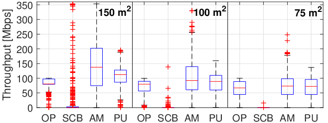
With the following experiment, we aim to identify what would be the optimal policy that a particular WLAN should adopt in order to increase its own throughput. In this case, we consider three rectangular maps (sparse, semi-dense and high-dense) with one WLAN (A) located at the center, and WLANs spread uniformly at random in the area (see Figure 12). Besides, we now consider that WLAN A has STAs.99 9 Note that the average results considering just one STA per WLAN are really similar to the ones presented in this work. Channel allocation (including the primary channel) is set uniformly at random to all the WLANs, except A. While the central WLAN is also set with a random primary channel, it is allocated the widest channel (i.e., ) in order to provide more flexibility and capture complex effects. While the DCB policies of the rest WLANs are picked uniformly at random (i.e., they will implement OP, SCB, AM or PU with same probability 1/4), A’s policy is set deterministically. Specifically, for each map sizes (i.e., 75, 100 and 150 m2), we generate deployments following the aforementioned conditions for each of the DCB policies that A can implement. That is, we simulate scenarios. The simulation time of each scenario is also seconds.

Figure 13 shows the average throughput experienced by A in the considered maps. The first noticeable result is that, in dense scenarios, SCB is non-viable for WLANs with wide allocated channels because they are most likely prevented to initiate transmissions. In fact, A is not able to successfully transmit any data packets in 61%, 84% and 99% of the scenarios simulated for SCB in the sparse, semi-dense and high-dense maps, respectively. Regarding the rest of policies, on average, A’s throughput is higher when implementing AM in all the maps. Especially, AM (and SCB in some cases) stands out in sparse deployment. Nevertheless, for dense deployments, there is a clear trend to pick just one channel when implementing AM or PU. That is why OP provides an average throughput relatively close to the ones achieved by these policies. Nonetheless, as the high standard deviation of the throughput indicates, there are important differences regarding among the evaluated scenarios. Table 5 compares the share of scenarios where AM or PU provide the highest individual throughput for A. We say that AM is better than PU if , and vice versa. We use the margin Mbps for capturing the cases where AM and PU perform similarly.
We see that in most of the cases AM performs better than PU. However, in some scenarios, PU outperforms AM. This improvement is accentuated for the high-density map, where a significant 57% (19% + 38%) of the scenarios achieve the same or highest throughput with PU. Also, there are a scenarios where the throughput experienced by PU with respect to AM is significantly higher (up to 61.5, 127.4 and 41.9 Mbps of improvement for the sparse, semi-dense and high-dense scenarios, respectively). This mainly occurs when the neighboring nodes occupy A’s primary channel through complex interactions caused by information asymmetries, keeping its backoff counter frozen for long periods of time. These are clear cases where adaptive policies could importantly improve the performance.
Therefore, as a rule of thumb for dense networks, we can state that, while AM reaches higher throughput on average, stochastic DCB is less risky and performs relatively well. Nonetheless, even though PU is fairer than AM on average, it does not guarantee the absence of starving WLANs either. It follows that WLANs must be provided with some kind of adaptability to improve both the individual throughput and fairness with acceptable certainty.
| Deployment | PU best | AM best | Draw |
|---|---|---|---|
| Sparse 150 m2 | 90/400 (23%) | 260/400 (65%) | 50/400 (13%) |
| Semi 100 m2 | 61/400 (15%) | 246/400 (62%) | 93/400 (23%) |
| High 75 m2 | 77/400 (19%) | 172/400 (43%) | 151/400 (38%) |
7 Conclusions
In this work, we show the effects on spatially distributed WLANs of different DCB policies, including a new approach that stochastically selects the transmission channel width. By means of modeling WLAN scenarios through CTMNs, we provide relevant insights such as the instantaneous vs. long-term throughput dilemma, i.e., always selecting the widest available channel found free does not always maximize the individual throughput. Besides, we show that often there is not an optimal global policy to be applied to each WLAN, but different policies are required, specially in non-fully overlapping scenarios where chain reaction actions are complex to foresee.
Simulations corroborate that, while AM is normally the optimal policy to maximize the individual long-term throughput, there are cases, particularly in high-density scenarios, where stochastic DCB performs better both in terms of individual throughput and fairness among WLANs. We conclude that the performance of DCB can be significantly improved through adaptive policies capable of leveraging gathered knowledge from the medium and/or via information distribution. In this regard, our next works will focus on studying machine learning based policies to enhance WLANs spectrum utilization in high-density scenarios.
Acknowledgment
This work has been partially supported by the Spanish Ministry of Economy and Competitiveness under the Maria de Maeztu Units of Excellence Programme (MDM-2015-0502), and by a Gift from the Cisco University Research Program (CG#890107, Towards Deterministic Channel Access in High-Density WLANs) Fund, a corporate advised fund of Silicon Valley Community Foundation. The work done by S. Barrachina-Muñoz is supported by a FI grant from the Generalitat de Catalunya.
Appendix A Dynamic channel bonding flowchart
In Figure 14, a simple flowchart of the transmission channel selection is shown.

Appendix B Optimal combination of DCB policies
Table 6 shows the individual and aggregated throughputs, and the Jain’s fairness index for all the combinations of DCB policies in Secnario IV.
| Policy | States | Throughput [Mbps] | Fairness | |||||
|---|---|---|---|---|---|---|---|---|
| AM | AM | AM | 5 | 199.96 | 3.58 | 199.96 | 403.49 | 0.67853 |
| (199.35) | (4.76) | (199.37) | (403.48) | (0.68247) | ||||
| AM | PU | AM | 10 | 149.41 | 62.45 | 149.41 | 361.27 | 0.89679 |
| (128.72) | (86.88) | (128.72) | (344.31) | (0.97131) | ||||
| PU | AM | PU | 14 | 109.84 | 108.44 | 109.84 | 328.12 | 0.99996 |
| (109.49) | (109.13) | (109.51) | (328.13) | (1.00000) | ||||
| AM | AM | PU | 9 | 111.31 | 106.91 | 110.33 | 328.55 | 0.99970 |
| (109.64) | (109.06) | (109.49) | (328.19) | (1.00000) | ||||
| AM | PU | PU | 12 | 111.29 | 106.94 | 110.33 | 328.56 | 0.99971 |
| (109.63) | (109.07) | (109.49) | (328.18) | (1.00000) | ||||
| PU | PU | PU | 14 | 109.85 | 108.44 | 109.85 | 328.13 | 0.99996 |
| (109.52) | (109.10) | (109.51) | (328.13) | (1.00000) | ||||
Appendix C Evaluation setup
The values of the parameters considered in the simulations are shown in Table 7. Regarding the path loss, we use the dual-slope log-distance model for 5.25 GHz indoor environments in room-corridor condition [32]. Specifically, the path loss in dB experienced at a distance is defined by
| (1) |
where m is the break point distance.
| Parameter | Description | Value |
| Central frequency | 5 GHz | |
| Basic channel bandwidth | 20 MHz | |
| Frame size | 12000 bits | |
| No. of frames in an A-MPDU | 64 | |
| Min. contention window | 16 | |
| No. of backoff stages | 5 | |
| MCS | 11ax MCS index | 0 - 11 |
| MCS’s packet error rate | 0.1 | |
| CCA | CCA threshold | -82 dBm |
| Transmission power | 15 dBm | |
| Transmitting gain | 0 dB | |
| Reception gain | 0 dB | |
| Path loss | see (1) | |
| Adjacent power leakage factor | -20 dB | |
| CE | Capture effect threshold | 20 dB |
| Background noise level | -95 dBm | |
| Empty backoff slot duration | 9 µs | |
| SIFS duration | 16 µs | |
| DIFS duration | 34 µs | |
| PIFS duration | 25 µs | |
| Legacy preamble | 20 µs | |
| HE single-user preamble | 164 µs | |
| Legacy OFDM symbol duration | 4 µs | |
| 11ax OFDM symbol duration | 16 µs | |
| Length of a block ACK | 432 bits | |
| Length of an RTS packet | 160 bits | |
| Length of a CTS packet | 112 bits | |
| Length of service field | 16 bits | |
| Length of MPDU delimiter | 32 bits | |
| Length of MAC header | 320 bits | |
| Length of tail bits | 18 bits |
The MCS index used for each possible channel bandwidth (i.e., 20, 40, 80 or 160 MHz) was the highest allowed according to i) the power power budget established between the WLANs and their corresponding STA/s, and ii) the minimum sensitivity required by the MCSs. As stated by the 11ax amendment, the number of transmitted bits per OFDM symbol used in data transmissions is given by the channel bandwidth and the MCS parameters, i.e., , where is the number of data sub-carriers, is the number of bits in a modulation symbol, is the coding rate, and is the number of single user spatial streams (note that we only consider one stream per transmission).
The number of data sub-carriers depends on the transmission channel bandwidth. Specifically, can be 234, 468, 980 or 1960 for 20, 40, 80, and 160 MHz, respectively. For instance, the data rate provided by MCS 11 in a 20 MHz transmission is Mbps. However, control frames are transmitted in legacy mode using the basic rate bits per OFDM symbol of MCS 0, corresponding to Mbps since the legacy OFDM symbol duration must be considered. With such parameters we can define the duration of the different packets transmissions, and the duration of a successful and collision transmission accordingly:
References
- [1] B. Bellalta. IEEE 802.11ax: High-efficiency WLANs. IEEE Wireless Communications, 23(1):38–46, 2016.
- [2] B. Bellalta, A. Checco, A. Zocca, and J. Barcelo. On the interactions between multiple overlapping WLANs using channel bonding. IEEE Transactions on Vehicular Technology, 65(2):796–812, 2016.
- [3] M. Park. IEEE 802.11ac: Dynamic bandwidth channel access. In Communications (ICC), 2011 IEEE International Conference on, pages 1–5. IEEE, 2011.
- [4] B. Bellalta, A. Faridi, J. Barcelo, A. Checco, and P. Chatzimisios. Channel bonding in short-range wlans. In European Wireless 2014; 20th European Wireless Conference; Proceedings of, pages 1–7. VDE, 2014.
- [5] S. Vasthav, S. Srikanth, and V. Ramaiyan. Performance analysis of an IEEE 802.11ac WLAN with dynamic bandwidth channel access. In Communication (NCC), 2016 Twenty Second National Conference on, pages 1–6. IEEE, 2016.
- [6] A. Faridi, B. Bellalta, and A. Checco. Analysis of Dynamic Channel Bonding in Dense Networks of WLANs. IEEE Transactions on Mobile Computing, 2016.
- [7] Sergio Barrachina-Muñoz, Francesc Wilhelmi, Ioannis Selinis, and Boris Bellalta. Komondor: a wireless network simulator for next-generation high-density wlans. In 2019 Wireless Days (WD), pages 1–8. IEEE, 2019.
- [8] L. Deek, E. Garcia-Villegas, E. Belding, S. Lee, and K. Almeroth. The impact of channel bonding on 802.11n network management. In Proceedings of the Seventh Conference on emerging Networking EXperiments and Technologies, page 11. ACM, 2011.
- [9] M. Y. Arslan, K. Pelechrinis, I. Broustis, S. V. Krishnamurthy, S. Addepalli, and K. Papagiannaki. Auto-configuration of 802.11n WLANs. In Proceedings of the 6th International Conference, page 27. ACM, 2010.
- [10] L. Deek, E. Garcia-Villegas, E. Belding, S. Lee, and K. Almeroth. Joint rate and channel width adaptation for 802.11 MIMO wireless networks. In Sensor, Mesh and Ad Hoc Communications and Networks (SECON), 2013 10th Annual IEEE Communications Society Conference on, pages 167–175. IEEE, 2013.
- [11] Y. Zeng, P. Pathak, and P. Mohapatra. A first look at 802.11 ac in action: Energy efficiency and interference characterization. In Networking Conference, 2014 IFIP, pages 1–9. IEEE, 2014.
- [12] M. X. Gong, B. Hart, L. Xia, and R. Want. Channel bounding and MAC protection mechanisms for 802.11ac. In Global Telecommunications Conference (GLOBECOM 2011), 2011 IEEE, pages 1–5. IEEE, 2011.
- [13] M. Kim, T. Ropitault, S. Lee, and N. Golmie. A Throughput Study for Channel Bonding in IEEE 802.11ac Networks. IEEE Communications Letters, 2017.
- [14] S. Barrachina-Muñoz, F. Wilhelmi, and B. Bellalta. To overlap or not to overlap: Enabling channel bonding in high-density WLANs. Computer Networks, 152:40 – 53, 2019.
- [15] M. Han, Sami K., L. X. Cai, and Y. Cheng. Performance Analysis of Opportunistic Channel Bonding in Multi-Channel WLANs. In Global Communications Conference (GLOBECOM), 2016 IEEE, pages 1–6. IEEE, 2016.
- [16] S. Khairy, M. Han, L. Cai, Y. Cheng, and Z. Han. A renewal theory based analytical model for multi-channel random access in ieee 802.11 ac/ax. IEEE Transactions on Mobile Computing, 2018.
- [17] P. Huang, X Yang, and L. Xiao. Dynamic channel bonding: enabling flexible spectrum aggregation. IEEE Transactions on Mobile Computing, 15(12):3042–3056, 2016.
- [18] A. Nabil, M. J. Abdel-Rahman, and A. B. MacKenzie. Adaptive Channel Bonding in Wireless LANs Under Demand Uncertainty. To appear in the Proceedings of the IEEE International Symposium on Personal, Indoor and Mobile Radio Communications (PIMRC), Montreal, QC, Canada, October 2017.
- [19] C. Kai, Y. Liang, T. Huang, and X. Chen. A Channel Allocation Algorithm to Maximize Aggregate Throughputs in DCB WLANs. arXiv preprint arXiv:1703.03909, 2017.
- [20] Y. Chen, D. Wu, T. Sung, and K. Shih. Dbs: A dynamic bandwidth selection mac protocol for channel bonding in ieee 802.11 ac wlans. In Wireless Communications and Networking Conference (WCNC), 2018 IEEE, pages 1–6. IEEE, 2018.
- [21] S. Byeon, H. Kwon, Y. Son, C. Yang, and S. Choi. Reconn: Receiver-driven operating channel width adaptation in ieee 802.11ac wlans. In IEEE INFOCOM 2018-IEEE Conference on Computer Communications, pages 1655–1663. IEEE, 2018.
- [22] P. Chatzimisios, A. Boucouvalas, and V. Vitsas. Performance analysis of IEEE 802.11 DCF in presence of transmission errors. In Communications, 2004 IEEE International Conference on, volume 7, pages 3854–3858. IEEE, 2004.
- [23] R. Boorstyn, A. Kershenbaum, B. Maglaris, and V. Sahin. Throughput analysis in multihop CSMA packet radio networks. IEEE Transactions on Communications, 35(3):267–274, 1987.
- [24] G. Bianchi. Performance analysis of the IEEE 802.11 distributed coordination function. IEEE Journal on selected areas in communications, 18(3):535–547, 2000.
- [25] B. Bellalta. Throughput Analysis in High Density WLANs. IEEE Communications Letters, 21(3):592–595, 2017.
- [26] B. Nardelli and E. Knightly. Closed-form throughput expressions for CSMA networks with collisions and hidden terminals. In INFOCOM, 2012 Proceedings IEEE, pages 2309–2317. IEEE, 2012.
- [27] S. C. Liew, C. H. Kai, H. C. Leung, and P. Wong. Back-of-the-envelope computation of throughput distributions in CSMA wireless networks. IEEE Transactions on Mobile Computing, 9(9):1319–1331, 2010.
- [28] B. Bellalta, A. Zocca, C. Cano, A. Checco, J. Barcelo, and A. Vinel. Throughput analysis in CSMA/CA networks using continuous time Markov networks: a tutorial. In Wireless Networking for Moving Objects, pages 115–133. Springer, 2014.
- [29] C. Kai, Y. Liang, T. Huang, and X. Chen. To bond or not to bond: An optimal channel allocation algorithm for flexible dynamic channel bonding in wlans. In Vehicular Technology Conference (VTC-Fall), 2017 IEEE 86th, pages 1–6. IEEE, 2017.
- [30] H. Salameh, M. Krunz, and D. Manzi. Spectrum bonding and aggregation with guard-band awareness in cognitive radio networks. IEEE Transactions on Mobile Computing, 13(3):569–581, 2014.
- [31] F Kelly. Reversibility and stochastic networks. Cambridge University Press, 2011.
- [32] D. Xu, J. Zhang, X. Gao, P. Zhang, and Y. Wu. Indoor office propagation measurements and path loss models at 5.25 GHz. In Vehicular Technology Conference, 2007. VTC-2007 Fall. 2007 IEEE 66th, pages 844–848. IEEE, 2007.