Structure of the flow and Yamada polynomials of cubic graphs

Using the interplay between classical and quantum polynomials of graphs and ideas from topological quantum field theory (TQFT), we establish results on the structure of the Yamada and flow polynomials of cubic graphs. It has been known since the work of Birkhoff and Lewis in the 1940s [3] that the values $(3\pm\sqrt{5})/2$ of the parameter play a special role in the theory of the chromatic polynomial ${\chi}_{T}$ of planar triangulations. In a series of papers [19, 20] in the 1960s, Tutte established further remarkable properties, including the golden identity. Formulated dually in terms of the flow polynomial $F_{G}$ of planar cubic graphs $G$, it reads

where $E$ is the number of edges of $G$ and ${\phi}$ denotes the golden ratio $(1+\sqrt{5})/2$. The special role played by ${\phi}+1$, and more generally by the Beraha numbers [2] $B_{n}=2+2{\rm cos}(2{\pi}/n)$, was conceptually explained in [6] where these results were placed in the context of ${\rm SO}(3)$ TQFT.

We show in Theorem 3.1 that Tutte’s identity (1.1) admits an extension to the Yamada polynomial $R_{G}$ of ribbon cubic graphs $G$ in ${\mathbb{R}}^{3}$:

where $V,E$ denote the number of vertices and edges of $G$, respectively. In fact, (1.2) is a common extension of (1.1) and of the identity for links, relating the $2$-colored Jones polynomial at $e^{{\pi}i/10}$ and the square of the Jones polynomial at $e^{-{\pi}i/5}$ [13, Corollary 4.16], see section 3.

The Yamada polynomial [24] is a quantum invariant of ribbon graphs [15] in ${\mathbb{R}}^{3}$, corresponding to the adjoint representation of $U_{q}({\mathfrak{so}}_{3})$. Conceptually, as discussed in [6, Section 5] and also [13, Section 4.4], the reasons underlying the golden identity are the level-rank duality between the ${\rm SO}(3)_{4}$ and the ${\rm SO}(4)_{3}$ TQFTs, and the isomorphism ${\mathfrak{so}}(4)\cong{\mathfrak{so}}(3)\times{\mathfrak{so}}(3)$.

Concretely, the Yamada polynomial is defined by the contraction-deletion rule and the $SO(3)$ Kauffman skein relation, see section 2.1 for details. For planar graphs $G$, the Yamada polynomial coincides with a renormalization of the flow polynomial:

For non-planar graphs (and for knotted embeddings of planar graphs) the Yamada polynomial carries a lot of information about the embedding of a ribbon graph in $3$-space, and so in general the Yamada polynomial of a ribbon graph and the flow polynomial of the underlying abstract graph are quite different.

In contrast with (1.1), in [1] we formulated a conjecture that the Tutte golden identity for the flow polynomial characterizes planarity of cubic graphs:

The inequality at the Galois conjugate values,

conjecturally also holds for any cubic graph $G$, with an equality if and only if $G$ is planar. In section 5 we prove the conjecture for a family of near-planar graphs (which have a planar projection with a single crossing); Conjecture 1.1 in general remains open.

It is interesting to note that as a consequence of (1.1), there is a relation between the values of the flow polynomial of planar cubic graphs at $0$ and $4$:

see lemma 4.1. More generally, a congruence $({\rm mod}\,5)$ between the values $R_{G}(-1)$, $R_{G}(1)$ implies an extension of (1.5) to all cubic graphs,

where the value $R_{G}(1)$ is also known as the Penrose number of $G$ (defined up to a sign), see section 4. Using these relations, we give an application to the structure $({\rm mod}\,5)$ of the flow polynomial at zero for cubic graphs. This value is known [4] to count Eulerian equivalence classes of totally cyclic orientations.

The proofs of the results in this paper are given in the context of the chromatic algebra [6], and more generally the ${\rm SO}(3)$ TQFT. Using these methods, we also answer a question of D. Treumann and E. Zaslow [16] about the asymptotics of the number of chromatic polynomials of planar triangulations, motivated by their work on Legendrian surfaces [17].

An exponential upper bound is well-known, and it can be deduced from Tutte’s enumeration of planar triangulations [18]. We show that the chromatic algebra contains a free semigroup, yielding an exponential lower bound, see section 6. Conceptually, this may be viewed as an application of the Tits alternative for semigroups.

The key ingredients used throughout the paper – the chromatic algebra and the flow category – are recalled in section 2. The identity (1.2) for the Yamada polynomial is established in section 3. Section 4 discusses the structure of the flow polynomial at zero $({\rm mod}\,5)$ and gives a proof of theorem 1.2. The proof of conjecture 5.1 for a collection of near-planar graphs is given in section 5. Since the original Tutte golden identity (1.1) serves as the motivation for several results in this paper, for convenience of the reader we include its proof in section 7.

This section summarizes the relevant background material and notation used in the paper.

The purpose of this section is to prove the extension (1.2) of the Tutte golden identity (1.1) to the Yamada polynomial of cubic ribbon graphs in ${\mathbb{R}}^{3}$. It is convenient to allow vertices of degree $2$ in the statement of the theorem:

If there are no vertices of degree $2$, then $E^{\prime}=E$, and (3.1) is the same identity as (1.2). Moreover, since both ${\chi}(G)$ and $V_{3}(G)$ are topological invariants of $G$, introducing new $2$-valent vertices (i.e. subdividing edges of $G$) does not affect (3.1).

In the special case where $G$ has no trivalent vertices, (3.1) gives an identity for the SO$(3)$ Kauffman polynomial of framed links in ${\mathbb{R}}^{3}$, where the factor $(-1)^{V-E}\,{\phi}^{E^{\prime}}$ equals $1$. Then the left-hand side of (3.1) may be interpreted as the $2$-colored Jones polynomial of the link, and the right-hand side equals the square of the Jones polynomial. Therefore for links, (3.1) matches the identity stated in [13, Corollary 4.16].

Proof of theorem 3.1. Recall from section 2.2 that if $G$ is planar, one has $F_{G}(Q)\,=\,(-1)^{V-E}\,R_{G}(q)$, where $Q=q+2+q^{-1}.$ In particular, for planar graphs $G$,

Therefore in this case, (3.1) is reduced to the Tutte golden identity (1.1).¹¹ 1 Its proof is given in section 7. In the general case of a ribbon graph $G$ in the statement of the theorem, the proof is by induction on the number $c$ of crossings in a planar diagram of $G$. The base case corresponds to planar graphs, discussed above.

As in section 2.7, the notation $[\!\begin{minipage}[43.36243pt]\includegraphics[scale={.17}]{circ.eps} \end{minipage}\hskip-25.00003pt_{\;q}$ in the proof below will denote the evaluation of the Yamada polynomial at $q$.

By induction assume that graphs with fewer than $c$ crossings satisfy (3.1). Consider a graph with $c$ crossings. For brevity of notation denote $x:=e^{2\pi i/10},y:=e^{-2\pi i/5}$. Combining the skein relation (2.5) with the contraction-deletion rule (2.3), one has

(3.2)

$${[\!\begin{minipage}[50.58878pt]\includegraphics[scale={.2}]{OverCrossing.eps} \end{minipage}\hskip-25.00003pt}_{\!\!x}=e^{2{\pi}i/10}\,{[\!\begin{minipage}[50.58878pt]\includegraphics[scale={.2}]{0ResFig.eps} \end{minipage}\hskip-25.00003pt}_{\!\!x}+{[\!\begin{minipage}[50.58878pt]\includegraphics[scale={.2}]{Ifig.eps} \end{minipage}\hskip-25.00003pt}_{\!\!x}+(e^{-2\pi i/10}-1)\,{[\!\begin{minipage}[50.58878pt]\includegraphics[scale={.2}]{1ResFig.eps} \end{minipage}\hskip-25.00003pt}_{\!\!x}.$$

Since the three graphs on the right have $c-1$ crossings, (3.1) holds for them by the inductive assumption, thus

(3.3)

$${[\!\begin{minipage}[50.58878pt]\includegraphics[scale={.2}]{OverCrossing.eps} \end{minipage}\hskip-25.00003pt}_{\!\!x}=(-1)^{V-E}{\phi}^{E^{\prime}}\left(e^{2{\pi}i/10}\,{[\!\begin{minipage}[50.58878pt]\includegraphics[scale={.2}]{0ResFig.eps} \end{minipage}\hskip-25.00003pt}_{\!\!y}^{\!2}-{\phi}^{3}{[\!\begin{minipage}[50.58878pt]\includegraphics[scale={.2}]{Ifig.eps} \end{minipage}\hskip-25.00003pt}_{\!\!y}^{\!2}+(e^{-2\pi i/10}-1)\,{[\!\begin{minipage}[50.58878pt]\includegraphics[scale={.2}]{1ResFig.eps} \end{minipage}\hskip-25.00003pt}_{\!\!y}^{\!2}\right).$$

Because of the normalization sign $(-1)^{V-E}$ in the formula relating the flow and Yamada polynomials of planar graphs, the linear relation (2.8) at $q=e^{-2\pi i/5}$ (corresponding to $Q={\phi}+1$) for the Yamada polynomial reads

(3.4)

$${[\!\begin{minipage}[50.58878pt]\includegraphics[scale={.2}]{Ifig.eps} \end{minipage}\hskip-25.00003pt}_{\!\!y}\,=\,-{\phi}^{-1}\,{[\!\begin{minipage}[50.58878pt]\includegraphics[scale={.2}]{0ResFig.eps} \end{minipage}\hskip-25.00003pt}_{\!\!y}+{\phi}^{-2}\,{[\!\begin{minipage}[50.58878pt]\includegraphics[scale={.2}]{1ResFig.eps} \end{minipage}\hskip-25.00003pt}_{\!\!y},$$

Applying this relation to ${[\!\begin{minipage}[50.58878pt]\includegraphics[scale={.2}]{Ifig.eps} \end{minipage}\hskip-25.00003pt}_{\!\!y}$ in (3.3) gives

(3.5)

$${[\!\begin{minipage}[50.58878pt]\includegraphics[scale={.2}]{OverCrossing.eps} \end{minipage}\hskip-25.00003pt}_{\!\!x}=(-1)^{V-E}{\phi}^{E^{\prime}}\left((e^{2{\pi}i/10}-{\phi})\,{[\!\begin{minipage}[50.58878pt]\includegraphics[scale={.2}]{0ResFig.eps} \end{minipage}\hskip-25.00003pt}_{\!\!y}^{\!2}+2\,{[\!\begin{minipage}[50.58878pt]\includegraphics[scale={.2}]{0ResFig.eps} \end{minipage}\hskip-25.00003pt}_{\!\!y}\,{[\!\begin{minipage}[50.58878pt]\includegraphics[scale={.2}]{1ResFig.eps} \end{minipage}\hskip-25.00003pt}_{\!\!y}+(e^{-2\pi i/10}-{\phi})\,{[\!\begin{minipage}[50.58878pt]\includegraphics[scale={.2}]{1ResFig.eps} \end{minipage}\hskip-25.00003pt}_{\!\!y}^{\!2}\right).$$

To prove the inductive step, one needs to show that (3.5) equals $(-1)^{V-E}{\phi}^{E^{\prime}}{[\!\begin{minipage}[50.58878pt]\includegraphics[scale={.2}]{OverCrossing.eps} \end{minipage}\hskip-25.00003pt}_{\!\!y}^{\!2}$. Using the skein relation (2.5) and the contraction-deletion rule,

(3.6)

$$(-1)^{V-E}{\phi}^{E^{\prime}}{[\!\begin{minipage}[50.58878pt]\includegraphics[scale={.2}]{OverCrossing.eps} \end{minipage}\hskip-25.00003pt}_{\!\!y}^{\!2}=(-1)^{V-E}{\phi}^{E^{\prime}}\left(e^{-2{\pi}i/5}\,{[\!\begin{minipage}[50.58878pt]\includegraphics[scale={.2}]{0ResFig.eps} \end{minipage}\hskip-25.00003pt}_{\!\!y}+{[\!\begin{minipage}[50.58878pt]\includegraphics[scale={.2}]{Ifig.eps} \end{minipage}\hskip-25.00003pt}_{\!\!y}+(e^{2\pi i/5}-1)\,{[\!\begin{minipage}[50.58878pt]\includegraphics[scale={.2}]{1ResFig.eps} \end{minipage}\hskip-25.00003pt}_{\!\!y}\right)^{2}.$$

To complete the proof, one replaces ${[\!\begin{minipage}[50.58878pt]\includegraphics[scale={.2}]{Ifig.eps} \end{minipage}\hskip-25.00003pt}_{\!\!y}$ with (3.4), and checks that the resulting expression matches (3.5). ∎

In this section we establish the $({\rm mod}\;5)$ version of the golden identity, and prove a theorem stated in the introduction:

Theorem 1.2. Let $G$ be a cubic graph with $V$ vertices. Then the value of the flow polynomial of $G$ at zero satisfies:

Moreover, suppose $G$ is a snark, that is a bridgeless cubic graph with chromatic index $4$. Then $F_{G}(0)\,\equiv 0\;({\rm mod}\,5)$, and therefore $F_{G}(0)$ is divisible by $120$.

Remark. [4, Theorem 1.2] interpreted $|F_{G}(0)|$ as the number of Eulerian equivalence classes of totally cyclic orientations.

Proof of theorem 1.2. We start by stating the $({\rm mod}\;5)$ version of the golden identity:

Proof of (4.3). The flow polynomial $F_{G}(Q)$ for $Q=(3-\sqrt{5})/2,(5-\sqrt{5})/2$ takes values in the ring $R={\mathbb{Z}}[\frac{1+\sqrt{5}}{2}]$. Consider the ideal $I$ generated by $\sqrt{5}$. Since ${\phi}\sqrt{5}=(5+\sqrt{5})/2\in I$, it follows that $1+{\phi}\equiv 4\;({\rm mod}\;\sqrt{5})$, and ${\phi}\equiv 3\;({\rm mod}\;\sqrt{5})$. Plugging this into the golden identity (1.1), one gets $F_{G}(0)\equiv 3^{E}F_{G}(4)^{2}\;({\rm mod}\;\sqrt{5})$. Since $F_{G}(0)$ and $3^{E}F_{G}(4)^{2}$ are integers, the equivalence holds $({\rm mod}\;5)$. ∎

Proof of (4.4). The values of the Yamada polynomial $R_{G}(e^{{\pi}i/5}),R_{G}(e^{-2{\pi}i/5})$ are elements of ${\mathbb{Z}}[{\zeta}_{5}]$, where ${\zeta}_{5}=e^{{\pi}i/5}$. Consider the ideal generated by $e^{{\pi}i/5}+1$. Modulo this ideal, $e^{{\pi}i/5}$ and $e^{-{\pi}i/5}$ are equivalent to $-1$, $e^{2{\pi}i/5}$ and $e^{-2{\pi}i/5}$ are equivalent to $1$, and ${\phi}=e^{{\pi}i/5}+e^{-{\pi}i/5}\equiv 3$. ∎

Remark. Another proof of lemma 4.1 may be given by following $({\rm mod}\;5)$ the steps of the proofs of the golden identities (1.1), (3.1). For example, the (mod $5$) version at $Q=4$ of the Tutte linear relation (2.8) for the flow polynomial of planar graphs, ${[\!\begin{minipage}[50.58878pt]\includegraphics[scale={.2}]{Ifig.eps} \end{minipage}\hskip-25.00003pt}_{\!\!{\phi}+1}={\phi}^{-1}{[\!\begin{minipage}[50.58878pt]\includegraphics[scale={.2}]{0ResFig.eps} \end{minipage}\hskip-25.00003pt}_{\!\!{\phi}+1}-{\phi}^{-2}{[\!\begin{minipage}[50.58878pt]\includegraphics[scale={.2}]{1ResFig.eps} \end{minipage}\hskip-25.00003pt}_{\!\!{\phi}+1}$, reads ${[\!\begin{minipage}[50.58878pt]\includegraphics[scale={.2}]{Ifig.eps} \end{minipage}\hskip-25.00003pt}_{\!\!4}\,\equiv\,2\;{[\!\begin{minipage}[50.58878pt]\includegraphics[scale={.2}]{0ResFig.eps} \end{minipage}\hskip-25.00003pt}_{\!\!4}+{[\!\begin{minipage}[50.58878pt]\includegraphics[scale={.2}]{1ResFig.eps} \end{minipage}\hskip-25.00003pt}_{\!\!4}$ $({\rm mod}\;5)$.

Returning to the proof of theorem 1.2, recall that for planar graphs $G$, $F_{G}(Q)\,=\,(-1)^{V-E}\,R_{G}(q)$, where $Q=q+2+q^{-1}.$ In particular, for planar $G$, $R_{G}(-1)\,=\,(-1)^{V-E}F_{G}(0)$. The following identity holds for the flow polynomial of all (planar and non-planar) graphs:

(4.5)

$${[\!\begin{minipage}[50.58878pt]\includegraphics[scale={.2}]{OverCrossing.eps} \end{minipage}\hskip-25.00003pt}_{\!\!0}\;=\;-{[\!\begin{minipage}[50.58878pt]\includegraphics[scale={.2}]{0ResFig.eps} \end{minipage}\hskip-25.00003pt}_{\!\!0}-{[\!\begin{minipage}[50.58878pt]\includegraphics[scale={.2}]{Xfig.eps} \end{minipage}\hskip-25.00003pt}_{\!\!0}-{[\!\begin{minipage}[50.58878pt]\includegraphics[scale={.2}]{1ResFig.eps} \end{minipage}\hskip-25.00003pt}_{\!\!0}.$$

This identity is checked by pairing both sides of (4.5) with the four basis elements of the flow category ${\mathcal{F}}^{Q}_{0,4}$ in figure 6. This relation coincides with the skein relation (2.5) for the Yamada polynomial, normalized by the factor $(-1)^{V-E}$, at $q=-1$. Thus $R_{G}(-1)\,=\,(-1)^{V-E}F_{G}(0)$ for all graphs $G$. Now it follows from (4.4) that for any abstract (planar or non-planar) cubic graph $G$,

Remark. Up to a sign, the value $R_{G}(1)$ of the Yamada polynomial of ribbon cubic graphs equals the Penrose number of $G$, introduced and studied in [14], [9, Section 2.3]. Indeed, the skein relation [9, Proposition 2], satisfied by the Penrose number, coincides with the version of the skein relation (2.5) for $(-1)^{V-E}R_{G}(1)$:

(4.7)

$${[\!\begin{minipage}[50.58878pt]\includegraphics[scale={.2}]{Ifig.eps} \end{minipage}\hskip-25.00003pt}_{\!\!1}={[\!\begin{minipage}[50.58878pt]\includegraphics[scale={.2}]{0ResFig.eps} \end{minipage}\hskip-25.00003pt}_{\!\!1}-{[\!\begin{minipage}[50.58878pt]\includegraphics[scale={.2}]{OverCrossing.eps} \end{minipage}\hskip-25.00003pt}_{\!\!1}.$$

It is an invariant of ribbon graphs where the ribbon structure affects only its sign, so $|R_{G}(1)|$ is an invariant of abstract cubic graphs.

The congruence (4.6), the relation $3V=2E$ for cubic graphs, and the fact that perfect squares are congruent to $0,1$, or $4$ $({\rm mod}\;5)$ conclude the proof of (4.1), (4.2).

To prove the last statement of the theorem, consider a planar diagram of a ribbon cubic graph $G$. In other words, the graph is immersed in the plane, with some edge crossings. The value $R_{G}(1)$ is independent of which strand is over/under in each crossing. Using the recursion relation (4.7) at $q=1$, one checks that $(-1)^{V-E}R_{G}(1)$ equals the signed count of $3$-edge colorings of $G$, where the sign gets a $(-1)$ factor for each pair of edges that cross with a different color. This is invariant of regular homotopy of the planar diagram, and it satisfies the skein relation: each $3$-coloring of the graph on the left in (4.7) corresponds (with the same sign) to a $3$-coloring of precisely one term on the right.

This implies that the Yamada polynomial of snarks at $q=1$ is zero. (More generally, there is a well-known correspondence between $3$-edge-colorings and $4$-flows, cf. Proposition 6.4.5 (ii) in [5], so for any cubic graph $|R_{G}(1)|\leq F_{G}(4)$, with equality for planar graphs.) Now the congruence $F_{G}(0)\,\equiv 0\;({\rm mod}\,5)$ follows from (4.6). Finally, since the flow polynomial $F_{G}(Q)$ of a snark is divisible by $\prod_{k=1}^{4}(Q-k)$, $F_{G}(0)$ is also divisible by $4!$. ∎

Unlike the golden identity for the Yamada polynomial, Theorem 3.1, which holds for any spatial cubic graph $G$, in [1] we stated a conjecture that the golden identity for the flow polynomial characterizes planarity:

In this section we develop methods to prove this conjecture for a certain family of non-planar cubic graphs. We will call a graph $G$ near-planar if it admits a planar projection with a single crossing, for example $K_{3,3}$ in figure 7. We will view such graphs as $G=[\!\begin{minipage}[50.58878pt]\includegraphics[scale={.2}]{OverCrossing.eps} \end{minipage}\hskip-25.00003pt\cup\overline{G}$ where $\overline{G}$ is a planar graph in a disk (the complement in $S^{2}$ of the shaded disk in figure 7) with $4$ endpoints on the boundary circle.

Considered as an element of the chromatic algebra $C^{Q}_{2}$, $\overline{G}$ may be expressed as a linear combination of the three basis elements without internal edges. The coefficients depend on $Q$; denote by ${\alpha},{\beta},{\gamma}$ their values at $Q=(3-\sqrt{5})/2$, figure 8. In the following lemma the graph $\overline{G}$ outside a disk will be fixed throughout the proof, and (as in section 2.7) the notation ${[\!\begin{minipage}[43.36243pt]\includegraphics[scale={.17}]{circ.eps} \end{minipage}\hskip-25.00003pt}_{\,Q}$ will stand for the evaluation of the flow polynomial at $Q$.

We remark that this lemma is motivated by D.W. Hall’s version of the golden identity for constrained chromials [8]. The proof of lemma 5.2 relies on the following statement.

The proof of proposition 5.3 amounts to checking that both sides have identical evaluations when paired up with the three basis elements $[\!\begin{minipage}[50.58878pt]\includegraphics[scale={.2}]{0ResFig.eps} \end{minipage}\hskip-25.00003pt$, $[\!\begin{minipage}[50.58878pt]\includegraphics[scale={.2}]{1ResFig.eps} \end{minipage}\hskip-25.00003pt$ and $[\!\begin{minipage}[50.58878pt]\includegraphics[scale={.2}]{Xfig.eps} \end{minipage}\hskip-25.00003pt$ of the chromatic algebra ${\mathcal{C}}^{Q}_{2}$. (As discussed in section 2.5, the bilinear pairing $\langle.\,,\,.\rangle_{Q}$ on $C_{2}^{Q}$ is non-degenerate precisely for $Q\neq(3\pm\sqrt{5})/2$.)

Proof of lemma 5.2. Setting $Q$ to equal $z=(5-\sqrt{5})/2$ in proposition 5.3 and using the contraction-deletion rule, one has the following equality:

(5.3)

$${[\!\begin{minipage}[50.58878pt]\includegraphics[scale={.2}]{OverCrossing.eps} \end{minipage}\hskip-25.00003pt}_{\!\!z}\,=\,\\ \frac{\phi}{2}\,{[\!\begin{minipage}[50.58878pt]\includegraphics[scale={.2}]{0ResFig.eps} \end{minipage}\hskip-25.00003pt}_{\!\!z}\,-\,\frac{{\phi}^{-1}}{2}\,{[\!\begin{minipage}[50.58878pt]\includegraphics[scale={.2}]{Ifig.eps} \end{minipage}\hskip-25.00003pt}_{\!\!z}\,+\,\frac{1}{2}\,{[\!\begin{minipage}[50.58878pt]\includegraphics[scale={.2}]{1ResFig.eps} \end{minipage}\hskip-25.00003pt}_{\!\!z}$$

Equation (5.2) is obtained by applying the golden identity (1.1) to the three planar cubic graphs on the right in (5.3). ∎

It follows from lemma 5.2 that conjecture 5.1 for near-planar graphs is equivalent to the inequality

(5.4)

$${[\!\begin{minipage}[50.58878pt]\includegraphics[scale={.2}]{OverCrossing.eps} \end{minipage}\hskip-25.00003pt}^{\!2}_{\!\!w}\,\leq\,{[\!\begin{minipage}[50.58878pt]\includegraphics[scale={.2}]{0ResFig.eps} \end{minipage}\hskip-25.00003pt}^{\!2}_{\!\!w}\,+\,{[\!\begin{minipage}[50.58878pt]\includegraphics[scale={.2}]{1ResFig.eps} \end{minipage}\hskip-25.00003pt}^{\!2}_{\!\!w}\,+\,{\phi}^{-1}\,{[\!\begin{minipage}[50.58878pt]\includegraphics[scale={.2}]{0ResFig.eps} \end{minipage}\hskip-25.00003pt}_{\!\!w}{[\!\begin{minipage}[50.58878pt]\includegraphics[scale={.2}]{1ResFig.eps} \end{minipage}\hskip-25.00003pt}_{\!\!w}\!.$$

We are now in a position to give a reformulation of conjecture 5.1 for near-planar graphs.

Proof. The term being squared on the right-hand side of (5.1) equals:

$$F_{G}(w)=\langle[\!\begin{minipage}[50.58878pt]\includegraphics[scale={.2}]{OverCrossing.eps} \end{minipage}\hskip-25.00003pt,\overline{G}\rangle_{w}=\langle[\!\begin{minipage}[50.58878pt]\includegraphics[scale={.2}]{OverCrossing.eps} \end{minipage}\hskip-25.00003pt,{\alpha}[\!\begin{minipage}[50.58878pt]\includegraphics[scale={.2}]{0ResFig.eps} \end{minipage}\hskip-25.00003pt+{\beta}[\!\begin{minipage}[50.58878pt]\includegraphics[scale={.2}]{1ResFig.eps} \end{minipage}\hskip-25.00003pt+{\gamma}[\!\begin{minipage}[50.58878pt]\includegraphics[scale={.2}]{Xfig.eps} \end{minipage}\hskip-25.00003pt\rangle_{w}$$

Analogous calculations for $[\!\begin{minipage}[50.58878pt]\includegraphics[scale={.2}]{0ResFig.eps} \end{minipage}\hskip-25.00003pt$ and $[\!\begin{minipage}[50.58878pt]\includegraphics[scale={.2}]{1ResFig.eps} \end{minipage}\hskip-25.00003pt$ in place of $[\!\begin{minipage}[50.58878pt]\includegraphics[scale={.2}]{OverCrossing.eps} \end{minipage}\hskip-25.00003pt$ yield

respectively. Equation (5.2) expresses the left-hand side in (5.1) in terms of ${[\!\begin{minipage}[50.58878pt]\includegraphics[scale={.2}]{0ResFig.eps} \end{minipage}\hskip-25.00003pt}_{\!\!w}$ and ${[\!\begin{minipage}[50.58878pt]\includegraphics[scale={.2}]{1ResFig.eps} \end{minipage}\hskip-25.00003pt}_{\!\!w}$. Multiplying out the resulting expressions, (5.1) is seen to be equivalent to (5.6). ∎

Next we establish the inequality (5.6) for an infinite family of near-planar graphs.

Examples of graphs, considered in this lemma, are shown in figure 10. The graph on the left, capped with ${[\!\begin{minipage}[50.58878pt]\includegraphics[scale={.2}]{OverCrossing.eps} \end{minipage}\hskip-25.00003pt}\!\!$, is $K_{3,3}$. An analogous proof shows that the inequality (1.4) at the Galois conjugate values ${\phi}+1$, ${\phi}+2$ also holds for the same family of graphs.

Proof of lemma 5.5. It suffices to prove that the inequality (5.6) is preserved under addition of a peripheral edge. We will also show that whenever the coefficients ${\alpha},{\beta},{\gamma}$ are non-zero, they satisfy

where $V$ is the number of vertices of $\overline{G}$. The result of adding a peripheral edge to $\overline{G}={\alpha}[\!\begin{minipage}[50.58878pt]\includegraphics[scale={.2}]{0ResFig.eps} \end{minipage}\hskip-25.00003pt+{\beta}[\!\begin{minipage}[50.58878pt]\includegraphics[scale={.2}]{1ResFig.eps} \end{minipage}\hskip-25.00003pt+{\gamma}[\!\begin{minipage}[50.58878pt]\includegraphics[scale={.2}]{Xfig.eps} \end{minipage}\hskip-25.00003pt\!\!$ is the graph $\overline{G}^{\prime}$ shown in figure 11. (There are $4$ possible peripheral edges; by symmetry between $\alpha$ and $\beta$ the proof below applies to each one.)

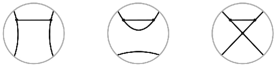
Applications of the contraction-deletion rule give

$$\overline{G}^{\prime}=-{\alpha}\,[\!\begin{minipage}[50.58878pt]\includegraphics[scale={.2}]{0ResFig.eps} \end{minipage}\hskip-25.00003pt+(-{\phi}{\beta}+{\gamma})\,[\!\begin{minipage}[50.58878pt]\includegraphics[scale={.2}]{1ResFig.eps} \end{minipage}\hskip-25.00003pt+({\alpha}-{\phi}^{2}{\gamma})\,[\!\begin{minipage}[50.58878pt]\includegraphics[scale={.2}]{Xfig.eps} \end{minipage}\hskip-25.00003pt\!\!.$$

Denote the coefficients of $\overline{G}^{\prime}$ by ${\alpha}^{\prime},{\beta}^{\prime},{\gamma}^{\prime}$:

This gives an inductive proof of the statement (5.7). A direct calculation shows that the desired inequality for the coefficients ${\alpha}^{\prime},{\beta}^{\prime},{\gamma}^{\prime}$ of $\overline{G}^{\prime}$,

is equivalent to

Since sign($\alpha$)$=$ sign($\beta)$, ${\phi}^{2}\,{\alpha}\,{\beta}\leq(1+3{\phi})\,{\alpha}\,{\beta}$.Therefore the assumed inequality (5.6) for ${\alpha},{\beta},{\gamma}$ implies the inequality (5.9) for ${\alpha}^{\prime},{\beta}^{\prime},{\gamma}^{\prime}$.

Finally, consider the last statement in conjecture 5.1. Note that the inequality ${\phi}^{2}\,{\alpha}\,{\beta}\leq(1+3{\phi})\,{\alpha}\,{\beta}$ in the previous paragraph is strict precisely when both ${\alpha},{\beta}$ are non-zero. Suppose the inductive construction of the family of graphs in the statement of the lemma starts with $[\!\begin{minipage}[50.58878pt]\includegraphics[scale={.2}]{Hfig.eps} \end{minipage}\hskip-25.00003pt$, and consider the first time a horizontal peripheral edge is added. Before this step, the graph $\overline{G}$ is of the form shown on the left in figure 12: there is a vertical line in the disk, intersecting the graph $\overline{G}$ in a single edge. The vector space of graphs in a disk with three boundary points, modulo the defining local relations of the chromatic algebra, is $1$-dimensional. Hence it is clear that $\overline{G}={\lambda}{[\!\begin{minipage}[50.58878pt]\includegraphics[scale={.2}]{Hfig.eps} \end{minipage}\hskip-25.00003pt}$ in ${\mathcal{C}}_{2}$, and the coefficient $\beta$ (defined in figure) 8 is zero.

Then adding a horizontal edge gives a scalar multiple of the graph on the right in figure 12, resulting in non-zero coefficients ${\alpha},{\beta}$. At this point, the graph $G={[\!\begin{minipage}[50.58878pt]\includegraphics[scale={.2}]{OverCrossing.eps} \end{minipage}\hskip-25.00003pt}\!\!\cup\overline{G}$ is still planar, since one of the crossing strands may be drawn within the rectangle in the graph on the right in the figure. Since both coefficients ${\alpha},{\beta}$ are non-zero, the addition of any new peripheral edge after this step makes the inequality (5.9) strict. (And of course the graph becomes non-planar.) It follows from (5.8) that all further additions of edges increase ${\alpha},{\beta}$ in absolute value, so the difference of the two sides of the inequality (5.9) continues strictly increasing. Thus the inequality detects planarity in this family of graphs. ∎

In this section we prove theorem 1.3, working dually with the flow polynomial of planar cubic graphs. Consider ${\mathcal{C}}^{Q}_{1,3}$, the vector space consisting of ${\mathbb{C}}$-linear combinations of planar cubic graphs in a rectangle with one marked point at the bottom and three marked points at the top of the rectangle, modulo the relations in figure 2. (This notion was also discussed at the end of section 2.6.) The loop value is $Q-1$, and for the remainder of this section we fix $Q=(3-\sqrt{5})/2$. As discussed in section 2.5, at this value of $Q$ there is an additional local relation

(6.1)

$$[\!\begin{minipage}[50.58878pt]\includegraphics[scale={.2}]{Ifig.eps} \end{minipage}\hskip-25.00003pt\,=\,-{\phi}\,[\!\begin{minipage}[50.58878pt]\includegraphics[scale={.2}]{0ResFig.eps} \end{minipage}\hskip-25.00003pt-{\phi}^{2}\,[\!\begin{minipage}[50.58878pt]\includegraphics[scale={.2}]{1ResFig.eps} \end{minipage}\hskip-25.00003pt.$$

${\mathcal{C}}^{Q}_{1,3}$ is a module over the chromatic algebra; the action is by vertical concatenation, matching three marked points on the boundary.

References

- [1] I. Agol and V. Krushkal, Tutte relations, TQFT, and planarity of cubic graphs, Illinois J. Math. 60 (2016), no. 1, 273-288.
- [2] S. Beraha, Infinite non-trivial families of maps and chromials, Thesis, Johns Hopkins University, 1975.
- [3] G.D. Birkhoff and D.C. Lewis, Chromatic polynomials, Trans. Amer. Math. Soc. 60 (1946), 355-451.
- [4] B. Chen and R. Stanley, Orientations, lattice polytopes, and group arrangements II: Modular and integral flow polynomials of graphs, Graphs Combin. 28 (2012), no. 6, 751-779.
- [5] R. Diestel, Graph theory. Graduate Texts in Mathematics, 173. Springer-Verlag, Berlin, 2005.
- [6] P. Fendley and V. Krushkal, Tutte chromatic identities from the Temperley-Lieb algebra, Geom. Topol. 13 (2009), 709-741.
- [7] P. Fendley and V. Krushkal, Link invariants, the chromatic polynomial and the Potts model, Adv. Theor. Math. Phys. 14 (2010) 2, 507–540.
- [8] D.W. Hall, On golden identities for constrained chromials, J. Combinatorial Theory Ser. B 11 (1971), 287-298.
- [9] F. Jaeger, On the Penrose number of cubic diagrams, Graph colouring and variations. Discrete Math. 74 (1989), 85-97.
- [10] V.F.R. Jones, Subfactors and knots. CBMS Regional Conference Series in Mathematics, 80. Published for the Conference Board of the Mathematical Sciences, Washington, DC; American Mathematical Society, Providence, RI, 1991.
- [11] L.H. Kauffman and P. Vogel, Link polynomials and a graphical calculus, J. Knot Theory Ramifications 1 (1992), 59-104.
- [12] P. Martin and D. Woodcock, The partition algebras and a new deformation of the Schur algebras. J. Algebra 203 (1998), no. 1, 91-124.
- [13] S. Morrison, E. Peters and N. Snyder, Knot polynomial identities and quantum group coincidences, Quantum Topol. 2 (2011), 101-156.
- [14] R. Penrose, Applications of negative dimensional tensors, 1971 Combinatorial Mathematics and its Applications (Proc. Conf., Oxford, 1969) pp. 221-244. Academic Press, London.
- [15] N.Yu. Reshetikhin and V.G. Turaev, Ribbon graphs and their invariants derived from quantum groups, Comm. Math. Phys. 127 (1990), 1-26.
- [16] D. Treumann, How many chromatic polynomials of planar maps are there?, https://mathoverflow.net/q/241734
- [17] D. Treumann and E. Zaslow, Cubic Planar Graphs and Legendrian Surface Theory, arXiv:1609.04892
- [18] W.T. Tutte, A census of planar maps, Canad. J. Math. 15 1963 249-271.
- [19] W.T. Tutte, On chromatic polynomials and the golden ratio, J. Combinatorial Theory 9 (1970), 289-296.
- [20] W.T. Tutte, More about chromatic polynomials and the golden ratio, Combinatorial Structures and their Applications, 439-453 (Proc. Calgary Internat. Conf., Calgary, Alta., 1969)
- [21] W.T. Tutte, A contribution to the theory of chromatic polynomials, Canadian J. Math. 6, (1954), 80-91.
- [22] K. Walker, Deletion-contraction relations, hard hexagons, and the shadow world, Talk at IPAM, 2007. Available at http://canyon23.net/math/talks/
- [23] H.Wenzl, On a sequence of projections, C. R. Math. Rep. Acad. Sci. Canada 9 (1987), 5-9.
- [24] S. Yamada, An invariant of spatial graphs, J. Graph Theory 13 (1989), 537- 551.