A clustering method for misaligned curves
Abstract
We consider the problem of clustering misaligned curves. According to our similarity measure, two curves are considered similar if they have the same shape after being aligned, and the warping function does not differ from the identity function very much. A clustering method is proposed, which updates curves so that similar curves become more similar, and then combines curves that are similar enough to form clusters. The proposed method needs to be used together with a clustering index and a set of combination thresholds. Simulation results are presented to demonstrate the performance of this approach under different parameter settings and clustering indexes. Two real data applications are included.
??
and
??
and
??
1 Introduction
Functional data are often observed over time and it is usual that a set of data curves show a common pattern with some variation in time. Before performing further analyses on data curves, such as estimating the common pattern, synchronizing the observed curves is necessary. Thus, curve alignment is an important problem in functional data analysis.
In the literature, many curve alignment methods have been proposed. One approach for curve alignment is landmark registration in Kneip and Gasser (1992). Landmarks are selected characteristics of curves, such as peaks or valleys. Another approach for curve alignment is continuous monotone registration, in which smooth monotone time transformations or warping functions are used to align individual curves to target curves. Curve alignment methods based on continuous monotone registration can be found in Silverman (1995), Ramsay and Li (1998), Kneip et al. (2000), Gervini and Gasser (2004), and Telesca and Inoue (2008). James James (2007) proposed a curve alignment method based on moments, which is a hybrid of the landmark approach and the continuous monotone registration approach.
In the past few years, some authors have investigated the clustering problem for misaligned curves. Tang and Müller (2009) proposed a two-step clustering method. In the first step, curves are aligned using estimated cluster-specific warping functions. In the second step, the aligned curves can be clustered using any existing clustering method, such as -means clustering or hierarchical clustering. In this method, it is assumed that the warping functions are non-linear and satisfy the boundary condition. Liu and Yang (2009) proposed the SACK model and provided an estimation procedure using the EM algorithm. Later, Sangalli et al. (2010) proposed a -means algorithm for clustering misaligned curves. In contrast to the approach in Tang and Müller (2009), in both Liu and Yang (2009) and Sangalli et al. (2010), linear warping functions are considered, and curve alignment and clustering are performed simultaneously, as summarized in Table 1.
| k-means | SACK | Two-step clustering | Our method | |
|---|---|---|---|---|
| Simultaneous clustering | ||||
| and alignment | Yes | Yes | No | Yes |
| Linear warping function | Yes | Yes | No | No |
In our option, it is better to perform alignment and clustering simultaneously. For instance, when we use the two-step clustering in Tang and Müller (2009), not all curves in the same cluster can be aligned well, as shown in Figure 5. It seems more efficient to perform alignment and clustering simultaneously. For using linear warping functions or nonlinear warping functions, we do not prefer one to the other and a suitable choice should be made based on the nature of data.
In this paper, we provide a method for clustering misaligned curves under the same assumptions for warping functions as in Tang and Müller (2009). For the proposed method, we include a parameter to adjust the penalty for large time variation. If it is desirable to put curves with different degrees of time variation into different groups, this can be done using a large . We organize this paper as follows. In Section 2, the details of this proposed method and theoretical result are given. Some results of simulation studies and analyses for two real data sets are presented in Sections 3 and 4. Discussion and suggestions are given in Section 5. Proofs are given in Section 6.
2 Methodology
In this section, we will first describe the set-up of the clustering problem and introduce the similarity measure in Section 2.1. Next, we give an overview of the proposed clustering process in Section 2.2. A theoretical result for curve updating is given in Section 2.3.
2.1 Similarity measure
We consider the problem of clustering data curves , , , where the curves are observed at time points . For , , and , , , let denote the observed value of curve at time point . We assume that these curves can be modelled as
where is called the shape function of curve and s are independent errors with mean zero. The goal of clustering is to assign curves into groups so that similar curves are in the same group, and the curve similarity measure will be introduced in this section.
For two curves with shape functions and that do not need to be aligned, a usual similarity measure is
where
, , and . Note that and means that the two curves with shape functions and have the same shape (up to a scale and level change).
Our curve similarity measure is based on the similarity measure for the warped curves, and we consider warping functions in the space
where is the space of continuously differentiable increasing functions defined on . The boundary constraint and can also be found in Ramsay and Silverman (1997) and is called the common endpoints condition in Tang and Müller (2009). Note that warping functions satisfying the boundary constraint cannot be linear unless they are equal to the identity function, and as such, we consider nonlinear warping functions.
Below we will define our curve similarity measure. For two curves with shape functions and , and for in , define
| (1) |
and , where is a non-negative parameter. Then, the similarity measure between and is defined as
Let , then we use as the warping function when aligning to and use as the warping function when aligning to .
Note that our similarity measure depends the parameter in (1). controls the degree of time variation. For a warping function , the integral implies that is the identity function. Using a large thus gives a large penalty for using warping functions that deviate from the identify function, and thus when the curves are clustered, the resulting time variation within the same group is expected to be limited. A similar penalty term for the warping function can be found in Section 5.4.2 in Ramsay and Silverman (1997). Some authors argue that in curve clustering, curve alignment is not always necessary if one would like to consider time variation as a clustering factor (Jacques and Preda (2014)). In that case, one can use a large in our similarity measure.
For convenience in evaluating the similarity measure, all data curves and warping functions are approximated using splines. We treat the approximate data curves as curves without errors and will not distinguish between the shape function of a data curve and the data curve itself hereafter.
2.2 Clustering method
In our clustering method, curves are updated so that curves that are similar enough become more similar and then eventually can be combined to form clusters. In the problem of clustering points, the idea of updating points can be found in Fukunaga and Hostetler (1975), Chen and Shiu (2007), and Shiu and Chen (2012). Chen and Shiu (2007, 2012) proposed a self-updating algorithm where points are moved toward their neighbors to form clusters automatically. Our approach is similar to Chen and Shiu’s approach since in both our method and Chen and Shiu’s algorithm, curves (or points) are updated using weighted averages. However, the weighting schemes are different. Our weighting scheme is based on Theorem 1 in Section 2.3.
To implement our clustering method, we need to choose a set of curve combination thresholds and a clustering index such as the Silhouette coefficient in Rousseeuw (1987). When contains several threshold values, we obtain the clustering result for each threshold value and then determine the final clustering result based on the clustering index. For most of our simulation studies, consists of 4 points near the 75% quantile of similarity measures of original curves excluding one’s. Below we describe our clustering method when has only one threshold value . First, we start an iterative process, where in each iteration, we perform
- (A)
curve combination and
- (B)
curve updating.
For curve combination, two curves can be combined if their similarity measure exceeds the given threshold . After curves are combined, curves will be updated. The iterative process stops when the average curve similarity measure remains stable. Note that at the end of this iterative process, it is possible that all curves are combined into one curve. To obtain a final clustering result from the whole iterative process, in each iteration, if some curves are combined in Step (A), then we obtain a candidate clustering result based on the updated curves after Step (A) and before Step (B) in that iteration. Thus at the end of the iterative process, several candidate clustering results are obtained, and the candidate result with the best clustering index is chosen as the final clustering result, where the clustering indexes are calculated based on the similarity measures of the original curves. The clustering procedure for a given combination threshold is given in Figure 1. Details for (B) curve updating, (A) curve combination and (C) obtaining a candidate clustering result in each iteration are given in Sections 2.2.1, 2.2.2 and 2.2.3 respectively.
2.2.1 Curve updating
In the curve updating step, suppose that we have several curves to be updated. Then curves are updated one at a time, and before each curve is updated, all curves are normalized so that their norms are equal to one. Let denote the curve to be updated and , , denote the rest curves. Then we update to
where , for , , and for , is the warping function in when aligning to .
To describe s, we introduce some notations. For , define for a real value function on . For two real valued functions and on , define
and . Then for , we set if
| (2) |
or
| (3) |
For the s that are nonzero, we choose s to be proportional to , where is the number of original curves that are updated/combined to form the curve ,
and is the maximum of the similarity measures that are less than 1 for the original data curves.
is computed based on the s. To obtain , let
then is the maximum of the following two quantities and :
| (4) |
and
| (5) |
where
, and .
2.2.2 Details for curve combination
We briefly state the tasks in the step of curve combination. In this step, we first put sets of similar curves into clusters, then for each cluster, align curves in the cluster to a reference curve, combine the aligned curves in the cluster to form a representative curve, and replace the curves in the cluster by the cluster representative. The representative curve is the fitted B-spline curve to the aligned data curves using weighted least square regression, where the reference curve for alignment is chosen as the curve in the cluster with the largest average of similarity measures to other curves in the cluster, and the weight for each curve in the weighted least square regression is the number of original curves that are updated/combined to form this curve. Here two curves are considered similar if their similarity measure exceeding .
The main difficulty in the step of curve combination is that sometimes we have a conflictive situation in clustering. For instance, suppose that we have a curve that is similar to two curves and , but and are not similar, then it is not clear how these three curves should be combined. In such case, we make use of the clustering index to help resolve this difficulty. Here the clustering index is computed based on the updated curves, not the original curves. For a combination result that assigns several updated curves to groups , , for combination, let denote the clustering index based on the updated curves.
Below we give the steps for assigning curves , , into clusters for combination.
- 1.
Compute
for .
- 2.
Sort the functions , , by s (from largest to smallest). Let be the sequence of sorted functions.
- 3.
Let be the first function in . Form a new group including by carrying out the steps (a)–(c) below and then remove the curves in from .
- (a)
Collect the functions s in that satisfy , and then sort these functions by s (from largest to smallest). Let be the sequence of the above sorted functions.
- (b)
Let , and then add the functions in to in turn under the constraint that each newly added function is similar to all functions in .
- (c)
For every function in , check whether it has similar function(s) outside .
- •
If it has no similar function outside , then is the new group containing .
- •
If it has similar function(s) outside , carry out (**) to update . The resulting is the new group containing .
- •
-
(**) For all functions in , determine in turn whether they will stay in according to the following criterion: for a function in , let be the collection of similar curves of and be the collection of curves that are similar to all curves in . Let , where is the complement of set . will stay in if either of the following two conditions are satisfied:
- (1)
is an empty set;
- (2)
, where is the most similar curve to among the curves in .
- (1)
- (a)
- 4.
Repeat 3 until is empty.
Following the above steps, we can assign , , into clusters and then combine curves in the same cluster.
2.2.3 Obtaining a candidate clustering result
In this section, we give details for obtaining a candidate clustering result (Step (C) in Figure 1). Note that in the curve combination step, we put some curves in clusters for combination and leave other curves outside those clusters, so we only have a partial clustering result. For curves that are not assigned into clusters for combination, we treat those curves as unassigned curves and then perform further clustering to obtain a complete clustering result as a candidate clustering result. The details are given below.
Let and be the collections of groups and unassigned curves respectively based on the partial clustering result in curve combination. Let be the number of groups in and be the number of unassigned curves in . Also, for a clustering result that assigns several updated curves to groups , , , let denote the similarity measure for the clustering result computed based on the original curves. Then we can obtain the candidate clustering result by carrying out the following steps for the case and .
- 1.
Set and .
- 2.
Suppose that is the collection of groups , , , and is nonempty. For every curve in , compute , , and . If the clustering result that includes has the largest value for some , then adds to group and removes it from .
- 3.
Suppose that after Step 2, remains nonempty and and becomes the collection of groups , , . For , , compute and let be the with the largest . Add the singleton to so that includes exactly groups: , , , . Remove from .
- 4.
Repeat the steps 2 and 3 until is empty.
- 5.
A complete clustering result is given by .
The above steps for obtaining a complete clustering result based on a partial clustering result characterized by a collection of non-singleton groups and a collection of unassigned curves can be viewed as a function of and . We will name this function cluster.1 and denote the function output by cluster.1(, ) based on input and . This function will be also used to handle the cases other than and .
For cases other than and , the details for obtaining a candidate clustering result based on the partial clustering result from curve combination are given below.
- •
and . Let and be the two curves in . If the two curves and are similar, then let be the clustering result including only one group . Otherwise, let be the clustering result of two singletons and .
- •
and . Suppose that .
-
(1) For , compute . Let be the curve with the largest and form a new group .
-
(2) Compute for , let be the curve with the largest for . Form the second group .
-
(3) Let cluster.1 .
- •
and . Let be the only group in the collection and be the only curve in . Suppose that is composed of curves , , . Compute and for , , . If some is larger than , put the curve into and let be the clustering result including exactly the group . Otherwise, let be the clustering result including exactly and the singleton group .
2.3 Curve updating - theoretical result
The weighting scheme in the curve updating step is based on our Theorem 1 in this section. The theorem gives some conditions on the weights when updating a curve to a weighted average of and warped versions of other curves , , :
where , for , , and for , is the warping function in when algning to . When the conditions in Theorem 1 hold, the updated curve is more similar to other curves than on average in the sense that (6) holds.
Theorem 1.
In our curve updating step, curves are normalized so that (C1) holds, only s satisfying (C2) will be used to update , weights s are selected so that (C3) and (C4) hold, and is chosen so that (C5) and (C6) hold. To specify s such that (C3) and (C4) hold, note that (C3) and (C4) are of the form for some known constants s. We simply set when for each to ensure that . The requirement for (C3) and (C4) corresponds to (2) and (3) respectively. There are certainly other ways for choosing s such that (C3) and (C4) hold, but we have not yet explored them.
In (2) and (3), and are residuals of projecting the warped curve to the space spanned by with respect to the semi-inner products and respectively. The effect for setting if (2) or (3) holds is so that curves that are very dissimilar to the residuals on average can be excluded, so that the updated curve can be more similar to the rest of the curves on average.
3 Simulation studies
In this section, we present results of the simulation studies under various settings with (the set of combination thresholds) taken to be the set : , 1, 2, 3 , where denotes the % sample quantile of the similarity measures of original curves that are less than one.
In Sections 3.1–3.3, we consider different types of warping functions using the Silhouette index as the clustering index and take for . Recall that for a warping function , we assume that is monotone on and satisfies the boundary condition
| (7) |
In Section 3.1, we consider warping functions satisfying the boundary condition (7) and the focus is on the effect of parameter and the unbalance class size. In Section 3.2, we consider warping functions that violate the boundary condition (7) slightly. In Section 3.3, we consider both linear and nonlinear warping functions to compare our method with the -means clustering method in Sangalli et al. (2010), which is designed for linear warping functions. The clustering results for the two methods are quite different, as expected.
In Section 3.4, we consider different values and different clustering index settings. The values considered are , , , and . For the clustering index, we try the Dunn index (Dunn (1974)) under different inter-cluster distances and intra-cluster distances to compare the results with those based on the Silhouette index.
In our simulation experiments, we use splines to approximation shape curves and warping functions. All data curves are first approximated using cubic splines, and the knots are selected using the method proposed by Zhou and Shen (2001) with one initial knot at 0.5. Then, we evaluate the approximated curves at 500 equally spaced points in to obtain the apprixomate observed curves and then perform shape curve approximation. For shape curve approximation, we use cubic splines with 16 equally spaced inner knots, and evaluate shape curves at 500 time points for finding fitted splines using the method of least squares. The shape curve approximation is also performed whenever a new shape curve is obtained during curve updating. For the approximation of warping functions, we use quadratic splines with three equally spaced inner knots. We also use quadratic splines with 23 equally spaced inner knots to approximate the inverse of warping functions.
3.1 Case of warping functions satisfying the boundary condition
We generate three sets of curves –. For , the -th set is composed of similar curves, which have a common shape function if properly warped. The shape functions for – are given below:
and
for . For the warping functions, we consider functions of the form , where so that the boundary condition holds. is either 10 or 20 in this study. For , we use warping functions , , , where for and , , 10. For , we use warping functions , , , , , . Every curve is generated with equally spaced time points , , , and the -th generated curve in the -th group is
| (8) |
where , , are IID . Here, or .
Note that , and thus if and curves are properly warped, they will have the same shape function. Figure 2 shows the three sets of curves without errors. It appears that curves in the same group follow a similar pattern since the time variation within each group is not very large. In contrast, for and curves , although they have the same shape function when properly warped, the unwarped curves for the two groups show quite different patterns due to large variation in time.

To investigate the effect of and class size, two values for and seven class sizes are considered, and the adjusted Rand indexes proposed by Hubert and Arabie (1985) for evaluating clustering results are calculated for the following two cases.
- (a)
There are two clusters and . This clustering case is denoted by .
- (b)
There are three clusters , , and . This clustering case is denoted by .
Table 2 shows the adjusted Rand index averages of 30 experiments for Cases (a) and (b), and the standard deviations are given in parentheses. Note that when , the shape functions for and curves are perfectly similar according to our similarity measure, and accordingly, our method usually returns the clustering result that matches Case (a). When , the shape functions for and curves are less similar since there is a penalty for using warping functions that are different from identity. As a result, our method often returns the clustering result matches Case (b). This phenomenon is observed under various combinations of class size and for each . In addition, the effect of class size is not significant.
| 1(0) | 0.5538(0) | 0.9802(0.1009) | 0.5513(0.0098) | ||
| 1(0) | 0.5185(0) | 0.9668(0.1448) | 0.5179(0.0035) | ||
| 1(0) | 0.7417(0) | 0.9984(0.0089) | 0.7403(0.0076) | ||
| 0.9974(0.0141) | 0.5172(0.0073) | 0.9974(0.0141) | 0.5185(0) | ||
| 0.9990(0.0057) | 0.6755(0) | 0.9984(0.0086) | 0.6745(0.0056) | ||
| 1(0) | 0.4096(0) | 0.9953(0.0179) | 0.4082(0.0056) | ||
| 1(0) | 0.6755(0) | 0.9816(0.0753) | 0.6730(0.0081) | ||
| 0.5538(0) | 1(0) | 0.5586(0.0363) | 0.9967(0.0125) | ||
| 0.5185(0) | 1(0) | 0.5138(0.0182) | 0.9992(0.0046) | ||
| 0.7417(0) | 1(0) | 0.7399(0.0097) | 0.9985(0.0082) | ||
| 0.5175(0.0058) | 0.9982(0.0098) | 0.5175(0.0058) | 1(0) | ||
| 0.6744(0.0062) | 1(0) | 0.6748(0.0036) | 0.9988(0.0063) | ||
| 0.4096(0) | 1(0) | 0.4090(0.0023) | 0.9977(0.0088) | ||
| 0.6755(0) | 1(0) | 0.6772(0.0154) | 0.9972(0.0091) | ||
3.2 Case of warping functions slightly violating the boundary condition
In this section, we examine the performance of our method when the boundary condition is violated slightly. We generate data using shape functions , , and in Section 3.1, but the warping functions are of the following forms:
and
where are generated from uniform distributions , , , and , , respectively. The range for is the same as in Section 3.1. Note that is a linear function, which is a common choice for warping functions, and is a function such that and . The two types of warping functions do not satisfy the boundary condition if and . For this part of simulation studies, we only consider and . The clustering results are shown in Table 3.
In Table 3, the adjusted Rand index averages for different combinations of warping functions and values are given for Cases (a) and (b). Due to the violation of the boundary condition, the clustering performance here is slightly different from when warping functions satisfy the boundary condition. However, for the effect of , the phenomenon observed in Section 3.1 is still present here. That is, our method returns results that match the case well when , and it returns results that match the case well when .
| 1(0) | 0.5538(0) | 0.9828(0.0939) | 0.5658(0.0652) | |
| 0.5538(0) | 1(0) | 0.5538(0) | 1(0) | |
3.3 Case of warping assumptions not holding
In this section, we compare the clustering result of our method with that of the -means clustering method in Sangalli et al. (2010), designed for linear warping functions, under two situations: (1) the warping functions are linear and (2) the warping functions satisfy the boundary condition. For our method, the warping assumption is violated in Case (1). For the -means method, the warping assumption is violated in Case (2). In what follows, the details of simulation data, clustering results , and some discussions are presented. We use the R package “fdama” to perform the -means clustering method in Sangalli et al. (2010).
First, we consider Case (1). In this experiment, we generate three groups of simulation curves – using random functions – given below, which are taken from Sangalli et al. (2010) with the modification that a linear function is used to transform the time range from to .
and
For each of –, 10 curves are generated using – respectively, but the random errors in are the same as those in and . The curves in and can be synchronized using linear warping functions. The graph of the data curves are shown in Figure 3(a).


For the -means clustering method, the curves can be clustered into two groups: and when the initial centers are specified properly. This result is expected since the curves in and can be synchronized by linear warping functions.
For our clustering method with , we obtain two groups: and . This clustering result is quite different from that of the -means method, because the curves in and have similar patterns when they are aligned using nonlinear warping functions satisfying the boundary condition. Figure 3(c) shows the warping functions when the curves in and are aligned to a reference curve and Figure 3 (b) shows the aligned curves. The curves in cannot be aligned well to the curves in or using warping functions satisfying the boundary condition, and as such, they are not clustered into one group under our method.
In the second experiment, we consider Case (2). We use shape functions
and warping functions to generate two groups of simulation curves and . Each group is composed of four curves with the same shape function, generated according to (8) but without errors.
In the second experiment, our clustering method with , gives the clustering result of two groups and . We also apply the -means clustering method in Sangalli et al. (2010) with the initial number of groups ranging from one to five.
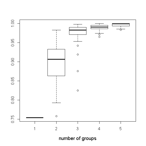
For a given number of clusters , we use every possible combination of curves among all data curves as initial cluster centers and obtain the average similarity measures between curves and their cluster centers for the corresponding clustering result. Figure 4 shows the box plot of averages of similarity measures for each . This figure shows that the median of averages of similarity measures increases as increases, and needs to be at least 3 for the averages of similarity measures to be less sensitive to the choice of initial cluster centers. The result for the -means method is quite different from that for our method since all the curves in (or ) cannot be aligned well to each other using linear warping functions.
In addition to the above experiments, we also tried the two-stage approach proposed in Tang and Müller (2009). In the first stage, the cluster-specific warping functions were estimated using our similarity measure. In the second stage, we used the function “kmeans.fd” in R package “fda.usc” to perform -means clustering to the aligned curves. The clustering results were not as good as ours in terms of the adjusted Rand index averages for the case. In addition, for the case and , the perfect clustering result is and our method gives the perfect result in all of the 30 trials. However, the two-stage approach gives the perfect result in only 13 of the 30 trials. Figure 5 shows the warped curves after the first-stage alignment using the two-stage approach. Note that the warped curves in show larger variation in time as compared to the warped curves in . As a result, -means clustering usually assigns the curves in into the same cluster, but fails to assign the curves in into the same cluster.

3.4 Effect of and clustering index
In this section, we investigate the influence of and clustering index on the proposed clustering method. The simulation data here are the same as those in the case in Section 3.1.
First, we apply the proposed method to the simulation data under different values. Table 4 shows the average Adjusted Rand index corresponding to five values under and . We find that the performance of the proposed method is still satisfactory when . When , the proposed method sometimes gives a large number of clusters. This is probably due to the fact that the curves cannot be combined in few iterations and the limit for the number of iterations is set to 10.
| 0.9728(0.1492) | 0.5538(0) | 0.6606(0.4551) | 0.5076(0.1112) | ||
| 1(0) | 0.5538(0) | 0.9986(0.0076) | 0.5538(0) | ||
| 1(0) | 0.5538(0) | 0.9986(0.0076) | 0.5538(0) | ||
| 1(0) | 0.5538(0) | 0.9986(0.0076) | 0.5538(0) | ||
| 1(0) | 0.5538(0) | 0.9931(0.0307) | 0.5538(0) | ||
| 0.5493(0.0251) | 1(0) | 0.4136(0.2027) | 0.9303(0.1702) | ||
| 0.5538(0) | 1(0) | 0.5523(0.0087) | 1(0) | ||
| 0.5538(0) | 1(0) | 0.5523(0.0087) | 1(0) | ||
| 0.5538(0) | 1(0) | 0.5523(0.0087) | 1(0) | ||
| 0.5538(0) | 1(0) | 0.5519(0.0088) | 1(0) | ||
Next, we apply the proposed method using the Dunn index to compare the clustering results with those based on the Silhouette index. The Dunn index based on groups , , is defined by
where and are inter-cluster distance and intra-cluster distance respectively. In this simulation study, we use three inter-cluster distances (I1)–(I3) and two intra-cluster distances (J1)–(J2) when evaluating the Dunn index. The definitions of these distances can be found in Soler et al. (2013) and stated below. In the following descriptions, denotes the distance between two elements and and denotes the number of elements in group .
- •
- (I1):
- (I2):
- (I3):
, where and
- (I1):
- •
- (J1):
- (J2):
, where and
- (J1):
In Table 5, we show the adjusted Rand index averages for the proposed method using Dunn index with the inter-cluster distances and intra-cluster distances mentioned above. Only the case is considered. We find that the Adjusted Rand index averages are similar for the six cases – , and the clustering results are very similar to the results based on Silhouette index.
| 1(0) | 1(0) | 0.9971(0.0159) | 1(0) | 0.9971(0.0159) | 1(0) | |
| 0.5538(0) | 0.5538(0) | 0.5538(0) | 0.5538(0) | 0.5538(0) | 0.5538(0) | |
| 0.5538(0) | 0.5538(0) | 0.5535(0.0019) | 0.5538(0) | 0.5535(0.0019) | 0.5538(0) | |
| 1(0) | 1(0) | 1(0) | 1(0) | 1(0) | 1(0) |
4 Data applications
In this section, we apply our method to two data sets using .
4.1 Berkeley growth study data
The Berkeley growth study data set (Tuddenham and Snyder (1954)) consists of the heights of 39 boys and 54 girls at 31 time points from when they were a year old to when they were 18 years old. Figure 6(a) shows these height curves, and Figure (b) shows the corresponding growth velocity curves that are obtained using the smoothing technique in Section 4.2 in Ramsay and Silverman (1997). In this analysis, we apply the proposed clustering method to the growth velocity curves instead of the original height curves. The height curves are increasing functions of age, and thus they inevitably form similar curves with . For convenience, we apply a linear function to transform the age range into .


Figure 7 shows the clustering results of these velocity curves from our clustering method with and . In both cases, these velocity curves are classified into two groups. We show the aligned velocity curves in Figures 7(a) and (c).
In Figures 7(a) and (c), for the curves in Group 2, the growth velocities at the end are greater than those in Group 1. It seems that the boys/girls whose growth curves are in Group 2 continued to grow higher at great speed at age 18 and their growth velocity curves show a different pattern since the growth processes were not yet complete. With , we found that Group 1 contains growth curves of boys and girls, but Group 2 contains growth curves of only boys. Figures 7 (b) and (d) show the warping functions for and 0.5. The warping functions for are smoother than those for , as expected.


4.2 Baby Finder data
A Baby Finder is an electronic device comprising a receiver and a transmitter, where the transmitter can send signals to the receiver continuously. The Baby Finder data set contains signal loss data for a Baby Finder from eight trials, provided by the third author of this paper. For each trial, the transmitter and the receiver are put together first and then are taken away along two paths respectively. If the moving path pairs for two trials are the same, we expect the corresponding signal loss curves to be similar.


Applying the proposed clustering method to those signal loss curves, the eight curves are clustered into three groups. The curves in the three groups are shown in Figures 8(a)–(c), respectively. The left figure shows the aligned six curves for the first group, all of which increase as time increases. The rest two curves have different patterns corresponding to different moving paths, and thus the two are clustered into two singleton groups. For each of the six curves in the first group, in addition to signal loss measurements, we have information on the travel distances of the receiver at different time points. We find that for the six trials, the signal losses at the same distance are about the same, and the maximum travel distances are the same, so we suspect that the receiver and the transmitter were taken away from the same pair of paths respectively for the six trials. The clustering results support our guess.
5 Discussion and suggestions
Based on our simulation results, the proposed method works well when warping functions satisfy the boundary condition. Regarding the implementation, one needs to choose , the penalty parameter and the clustering index. Below are our comments and suggestions when is determined using .
- •
When is small, it takes very few iterations for the curves to be combined, but curves that are not very similar may be combined and may be put into the same cluster due to the small combination threshold values. As increases, it can be ensured that only similar curves are combined but it takes more iterations for the curves to be combined. Based on our simulation experiments, the clustering results remain stable when is between and . If is too large, the curves may not be combined in the limited number of iterations and one may have to increase the limit for the number of iterations, and computation time can be longer. Our suggestion is to choose a large (as large as possible, but not large enough to make the number of iterations reaches its limit).
- •
In most of our simulation experiments, we use , and the computation takes a lot of time. For the case and in Table 1, the median compuation times (three trials) for and are 22142 seconds and 7574 seconds respectively using a machine with Intel CPU i7-4790K. For the case where , , , the median compuation times (three trials) is 11133 seconds. If we use , for the case where , , , the median compuation time (three trials) becomes 3970 seconds, which is much less than that of the case with .
- •
The choice of depends on to what extent time variation is considered as a clustering factor. Consider the case where one curve can be perfectly aligned to another curve using a warping function , but is very different from the identity function. In such case, if one would like and to be assigned into the same cluster (time variation is not important), then should be set to 0. Otherwise, a nonzero should be used. Using a large means that time variation is considered as an important factor in clustering.
- •
Since the results based on the Dunn index are very similar to those based on the Silhouette index, the effect of clustering index does not seem to be significant. If one would like to choose a clustering index, it is recommended to use a clustering index that does not involve cluster centers (such as the Silhouette coefficient or the Dunn index) since the proposed method does not compute cluster centers in the clustering process.
6 Proofs
In the section, we give the proof of Theorem 1, and the proofs of two facts: Facts 1 and 2, which are used in the proof of Theorem 1. We will state and prove Facts 1 and 2 first.
We first state Fact 1. Let . Below are the assumptions, statement and proof of Fact 1.
- (A1)
Suppose that , , and , where s are constants in such that .
- (A2)
Suppose that for , , , is a positive semi definite symmetric bilinear form from to .
- (A3)
For , , , let be the semi-norm on defined by for .
- (A4)
Suppose that for , , .
- (A5)
Suppose that , , are positive constants.
Fact 1.
Suppose that (A1)–(A5) hold. For , let
and
Let , , , , and
If and
| (9) |
then .
To find a lower bound for the expression
we consider the Taylor expansion of at , which gives
where is between and . Apply the result from Taylor expansion with and we have
| (10) | |||||
where . Suppose that (9) holds, then , using the fact that , we have
which implies that and . It then follows from (9) and (10) that
Thus for , . Therefore, when (9) holds. The proof of Fact 1 is complete.
Next, we give the assumptions, statement and proof of Fact 2.
- (A6)
Suppose that is a positive semi definite symmetric bilinear form from to .
- (A7)
Let be the semi-norm on defined by for .
- (A8)
Suppose that for , , .
Fact 2.
Suppose that (A1) and (A6)–(A8) holds. Let . For , let
and
Let
and
If for every , , and
| (11) |
then .
Proof of Fact 2. Let , then
Under the conditions that , for every and , we have and
so
The proof of Fact 2 is complete.
Next, we provide the proof of Theorem 1 as follows.
Proof of Theorem 1. To establish
| (12) |
we will prove
| (13) |
and
| (14) |
Then
and (12) holds.
References
- Chen and Shiu (2007) T.-L. Chen and S.-Y. Shiu. A new clustering algorithm based on self-updating process. In Proceedings of the American Statistical Association, Statistical Computing Section [CD-ROM], Salt Lake City, Utah. (2007).
- Dunn (1974) J. C. Dunn. Well separated clusters and optimal fuzzy partitions. Journal of Cybernetics, 4:95–104 (1974).
- Fukunaga and Hostetler (1975) K. Fukunaga and L. D. Hostetler. The estimation of the gradient of a density function, with applications in pattern recognition. IEEE Transactions on Information Theory, 21:32–40 (1975).
- Gervini and Gasser (2004) D. Gervini and T. Gasser. Self-modelling warping functions. Journal of the Royal Statistical Society, Series B: Statistical Methodology, 66:959–971 (2004).
- Hubert and Arabie (1985) L. Hubert and P. Arabie. Comparing partitions. Journal of Classification, 2:193–218 (1985).
- Jacques and Preda (2014) J. Jacques and C. Preda. Functional data clustering: a survey. Advances in Data Analysis and Classification, 8:231–255 (2014).
- James (2007) G. M. James. Curve alignment by moments. The Annals of Applied Statistics, 1:480–501 (2007).
- Kneip and Gasser (1992) A. Kneip and T. Gasser. Statistical tools to analyze data representing a sample of curves. The Annals of Statistics, 20:1266–1305 (1992).
- Kneip et al. (2000) A. Kneip, X. Li, K. B. MacGibbon, and J. O. Ramsay. Curve registration by local regression. The Canadian Journal of Statistics/La Revue Canadienne de Statistique, 28:19–29 (2000).
- Liu and Yang (2009) X. Liu and M. C. Yang. Simultaneous curve registration and clustering for functional data. Computational Statistics & Data Analysis, 53:1361–1376 (2009).
- Ramsay and Li (1998) J. O. Ramsay and X. Li. Curve registration. Journal of the Royal Statistical Society, Series B: Statistical Methodology, 60:351–363 (1998).
- Ramsay and Silverman (1997) J. O. Ramsay and B. W. Silverman. Functional Data Analysis. Springer-Verlag Inc (1997). ISBN 0-387-94956-9.
- Rousseeuw (1987) P. J. Rousseeuw. Silhouettes: A graphical aid to the interpretation and validation of cluster analysis. Journal of Computational and Applied Mathematics, 20:53 – 65 (1987).
- Sangalli et al. (2010) L. M. Sangalli, P. Secchi, S. Vantini, and V. Vitelli. -mean alignment for curve clustering. Computational Statistics & Data Analysis, 54:1219–1233 (2010).
- Shiu and Chen (2012) S.-Y. Shiu and T.-L. Chen. Clustering by self-updating process. In arxiv:1201.1979 (2012).
- Silverman (1995) B. W. Silverman. Incorporating parametric effects into functional principal components analysis. Journal of the Royal Statistical Society, Series B: Methodological, 57:673–689 (1995).
- Soler et al. (2013) J. Soler, F. Tencé, L. Gaubert, and C. Buche. Data clustering and similarity. In Proceedings of the Twenty-Sixth International Florida Artificial Intelligence Research Society Conference, pages 492–495, St. Pete Beach, Florida. (2013).
- Tang and Müller (2009) R. Tang and H.-G. Müller. Time-synchronized clustering of gene expression trajectories. Biostatistics, 10:32–45 (2009).
- Telesca and Inoue (2008) D. Telesca and L. Y. T. Inoue. Bayesian hierarchical curve registration. Journal of the American Statistical Association, 103:328–339 (2008).
- Tuddenham and Snyder (1954) R. D. Tuddenham and M. M. Snyder. Physical growth of california boys and girls from birth to eighteen years. In University of Califormia Publications in Child Development, volume 1, pages 183–364. University of California Press (1954).
- Zhou and Shen (2001) S. Zhou and X. Shen. Spatially adaptive regression splines and accurate knot selection schemes. Journal of the American Statistical Association, 96:247–259 (2001).