August 24, 2026
A quantum hydrodynamical description for scrambling and many-body chaos
Abstract
Recent studies of out-of-time ordered thermal correlation functions (OTOC) in holographic systems and in solvable models such as the Sachdev-Ye-Kitaev (SYK) model have yielded new insights into manifestations of many-body chaos. So far the chaotic behavior has been obtained through explicit calculations in specific models. In this paper we propose a unified description of the exponential growth and ballistic butterfly spreading of OTOCs across different systems using a newly formulated “quantum hydrodynamics,” which is valid at finite and to all orders in derivatives. The scrambling of a generic few-body operator in a chaotic system is described as building up a “hydrodynamic cloud,” and the exponential growth of the cloud arises from a shift symmetry of the hydrodynamic action. The shift symmetry also shields correlation functions of the energy density and flux, and time ordered correlation functions of generic operators from exponential growth, while leads to chaotic behavior in OTOCs. The theory also predicts an interesting phenomenon of the skipping of a pole at special values of complex frequency and momentum in two-point functions of energy density and flux. This pole-skipping phenomenon may be considered as a “smoking gun” for the hydrodynamic origin of the chaotic mode. We also discuss the possibility that such a hydrodynamic description could be a hallmark of maximally chaotic systems.
I Introduction
Chaotic phenomena are ubiquitous in nature. While much has been learned about chaos at a classical level, its characterizations and manifestations at a quantum level are far less understood, especially in many-body systems.
One characterization of chaos in quantum many-body systems is the Eigenstate Thermalization Hypothesis (ETH) [1, 2, 3, 4, 5] which says that for a chaotic system, highly excited energy eigenstates should behave like a thermal state. ETH is a powerful statement, implying that chaos underlies thermodynamical behavior of an isolated quantum statistical system. But it is not easy to work with or to check explicitly in practice as energy eigenstates of many-body systems are hard to come by.11 1 See also [6] for a recent proposal for another manifestation of quantum chaos in many-body systems. More recently, studies of out-of-time ordered thermal correlation functions in holographic systems and in solvable models like Sachdev-Ye-Kitaev (SYK) model have yielded new insights into manifestations of many-body chaos [11, 8, 7, 9, 12, 10, 15, 13, 14, 16, 17, 18, 19].
More explicitly, consider a quantum many-body system at a finite temperature , and the expectation value of the square of the commutator of two generic few-body operators and
| (1) | |||
| (2) | |||
| (3) |
where and are respectively referred to as the time ordered (TOC) and out-of-time ordered (OTOC) correlation functions.

For convenience throughout the paper we will assume that both and are normalized such that they can be considered as dimensionless. When is small, should be very small,
| (4) |
where denotes the total number of degrees of the system and is the characteristic relaxation time of the thermal equilibrium. For a chaotic large theory one typically expects that will grow exponentially with time
| (5) |
until the so-called scrambling time when becomes of . The Lyapunov exponent has been shown to be bounded in a generic system by [10] (below we will set and to throughout the paper)
| (6) |
Physically one can interpret the behavior (5) as due to scrambling. At operator involves only a few degrees of freedom. Under time evolution, expands in the space of degrees of freedom, i.e. it gets scrambled among more and more degrees of freedom. keeps increasing until is scrambled essentially among all degrees of freedom, when becomes and saturates (See Fig. 1). The exponential behavior (5) reflects that the scrambling procceds at a steady rate with .
When we separate and also spatially, then at large distances (5) appears to generalize to
| (7) |
where in (7) is often referred to as the butterfly velocity which characterizes the scrambling/expansion of an operator in space. Equation (7) is observed in a SYK chain and essentially all holographic systems [8, 9, 20]. In other systems different forms of spatial propagation are often seen instead [23, 22, 21]. For instance in [23, 22] chaos is described by a diffusive spreading around the exponential growth22 2 In [20, 9], the behavior below has been observed as transient behavior to (7).
| (8) |
There have also been studies using random unitary circuits which find other types of butterfly spreading, but not a nonzero Lyapunov exponent [24, 25].
The behaviors (5)–(8) have been found in many model systems, often through complicated model specific calculations. A unified understanding of how they emerge across different systems is still lacking. It is the purpose of this paper to propose such an effective description which does not depend on details of a specific system. We will be interested in those systems for which , so that the chaotic behavior is intrinsically quantum, i.e. does not have a straightforward semi-classical limit.

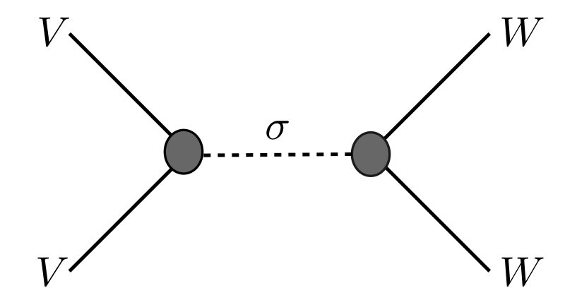

For such systems we propose the following effective description of chaos:
- A.
To leading order in the limit , the scrambling of a generic few-body operator in a chaotic system allows a coarse-grained description in which the growth of the operator can be understood as building up a “cloud” of some effective field . More explicitly, as indicated in Fig. 2, can be represented by a core operator , which involves the degrees of freedom originally in , dressed by a variable .
- B.
In this paper we will realise the above elements through developing a “quantum hydrodynamic” theory for chaos in which we identify with the hydrodynamic mode for energy conservation. As we will shortly discuss, this connection between the effective chaos mode and hydrodynamics can be motivated from the explicit calculations of OTOCs in holography and SYK models. Our general hydrodynamic theory not only provides a system-independent explanation of the chaotic behavior (5)–(8) of OTOCs, but also leads to new predictions which can be explicitly checked. As we will remark later in the paper, likely the full content of this hydrodynamic theory only applies to systems which are maximally (or nearly maximally) chaotic. Nevertheless, we expect that various features associated with items A and B above may also apply to non-maximal chaotic systems. So throughout the paper we use a general Lyapunov exponent unless explicitly stated.
There have been various hints for such an effective description, and possible connection with hydrodynamics. In holographic systems, the scrambling and chaotic behaviors are realized through the backreaction of an in-falling particle to the spacetime geometry [7, 9, 8] which can be interpreted in the boundary theory as building up a hydrodynamic cloud, see Fig. 4. In SYK, chaos is captured by a low energy effective action, the Schwarzian [11, 17, 13, 15, 14, 16, 18, 19]. As already pointed out by K. Jensen [14], the Schwarzian can be considered as the effective action for a hydrodynamic mode associated with energy conservation (i.e. the variable mentioned above). In fact, Fig. 2 and Fig. 3 have been implicit in various calculations performed using Schwarzian in [15] (see also [17]) for SYK. Here we propose that they should apply to general chaotic systems. Note the construction of the Schwarzian action from gravity [15] parallels that of construction of hydrodynamic action in [27, 26, 28]. Furthermore, [22] extracted an unstable “chaotic mode” by developing a kinetic theory for OTOCs. Finally in many holographic examples and non-holographic models the butterfly velocity in (7) and in (8) appear to be related to the thermal/energy diffusion constant (for example see [29, 30, 31, 32, 33, 20, 21, 23]). Given that hydrodynamic degrees of freedom constitute a universal sector among all quantum many-body systems, it is then natural to search for a hydrodynamic origin of the chaotic behavior (5)–(8) (see also [36, 37, 35] for other attempts to connect chaos and hydrodynamics).
Despite the above hints, at first sight there are nevertheless various important difficulties for a hydrodynamic description of chaotic behavior (5)–(8). We now discuss these difficulties and how to address them to help clarify and elaborate on our proposal:
- 1.
Chaotic behavior lies outside the usual range of validity of hydrodynamics.
Conventionally hydrodynamics is formulated as a low energy effective theory for gapless modes associated with conserved quantities, valid for time variation scales much larger than typical relaxation scales , which for illustrative purposes we will take to be of order (e.g. in a strongly coupled system). It is written using a derivative expansion with expansion parameter . Such a description is inadequate for our purpose,33 3 Of course in the standard hydrodynamic limit , the hydrodynamic equations can exhibit chaotic behavior, such as turbulence. These infrared chaotic behavior has a smooth classical limit and has nothing to do with what we discuss in the paper which may be considered as ultraviolet chaos from hydrodynamics perspective. as in (5) the Lyapunov exponent is often of order . Hence to capture the exponential growth (5) one needs a formulation which is valid for . Furthermore since we interested in quantum systems in which is proportional to , one needs a formulation which applies at quantum level with a finite , rather than the classical statistical limit which is normally taken.
A quantum hydrodynamics which applies to the regime can be obtained using the action formalism recently developed in [38, 39].44 4 See also [40, 41] for discussions of extracting linearized hydrodynamic constitutive relations to all derivative orders from holography. The theory should be understood as obtained from integrating out all degrees of freedom of a quantum many-body system except for those associated with conserved quantities. It can be nonlocal, but non-locality is only at scales of order .55 5 For example it can incorporate quasi-normal modes. This is due to the fact that for a generic system at a finite temperature, hydrodynamical modes are the only gapless degrees of freedom, thus the integrated out modes have energies or decay rates at least of order . Working with such a theory is delicate as physics at scales of order depends on microscopics of individual systems, which makes extracting universal information challenging. Nevertheless we will see that significant amount of universality can be obtained.
In particular, for the purpose of describing the chaotic behavior at leading order in it is enough to work to quadratic order in perturbations from thermal equilibrium. Since the chaotic mode is only associated with energy conservation, to minimize technicalities in this paper we will consider a theory whose only conserved quantity is energy conservation. Such a theory describes either a -dimensional quantum mechanical system or a higher dimensional system with strong momentum dissipation at some microscopic scales. It should be straightforward, although technically more cumbersome, to write down a theory which has full energy-momentum conservation or other conserved quantities, which will be left for future work.
Figure 5: Chaos is described in our framework through a pole (at ) in the upper half complex frequency plane of the retarded Green function of hydrodynamic variable . Such a pole does not indicate an instability, since it originates from a symmetry of the quantum hydrodynamics. - 2.
Can hydrodynamics of a stable system have an exponentially growing mode?
More explicitly, if exponential growth (5) arises from exchanging and propagation of hydrodynamic variable associated with energy conservation, would that immediately lead to inconsistencies as the stress tensor certainly cannot have such exponential behavior? It turns out they can be perfectly consistent.
We propose that the quantum hydrodynamics for a chaotic system possesses a shift symmetry. On the one hand, this shift symmetry warrants that the retarded Green’s function of has a pole in the upper half complex frequency plane for real momentum as indicated in Fig. 5, which leads to exponentially growing behavior in real time. On the other hand, the structure of the quantum hydrodynamics is such that precisely the same symmetry ensures that such an exponential mode is invisible to the full stress tensor, and the retarded Green’s functions of the stress tensor components have poles only in the lower half complex frequency plane for real .
Figure 6: Left: The hydrodynamic theory in a state is formulated directly in real time on the CTP contour. Right: OTOCs (3) require a contour of four segments. - 3.
In [38, 39] the hydrodynamics action is formulated as an effective theory for a system in some state defined on the closed time path (CTP), see Fig. 6. How can a theory which is formulated on a closed time path, i.e. on a contour with two segments, describe the chaotic behavior of OTOCs, which require a contour of four segments?
The reason is simple. To leading order in , only two-point functions of field are needed, as indicated in Fig. 3. Thus OTOCs on a 4-contour in the end reduce to a sum of two-point functions of on a two-contour which are in turn determined by the quantum hydrodynamics, see Fig. 7. In particular, the difference between the TOCs of (2) and OTOCs of (3) lies in the precise structure of respective effective vertices, see Fig. 3. In TOCs, due to the shift symmetry in the coupling between the core operator and its hydrodynamic dressing, the contributions of exponentially growing mode cancel while in OTOCs exponential mode survives and leads to (5)–(8).
Figure 7: At leading order in large OTO four-point functions defined on a four-contour reduce to a sum of two-point functions of . They can therefore be calculated from the effective action of the hydrodynamic field on a CTP contour. - 4.
Why does chaotic behavior have anything to do with energy conservation?
Despite the aforementioned hints it is certainly not clear to what extent chaos should always be related to the hydrodynamic mode associated to energy conservation. For instance it is certainly the case that driven systems, in which energy conservation can be badly broken, can also be chaotic. Chaos has also been studied using random unitary circuits [24, 25] which do not have energy conservation. A possible explanation is that such a connection may be a feature of systems which are or are close to being maximally chaotic. We will elaborate more on this point in the conclusion section.
Now that we have motivated our hydrodynamic description of chaos we can describe the implications of such an effective theory. In particular, a key feature of this theory is that the mode which characterizes the energy conservation also describes the chaotic growth of general operators. This dual role leads to interesting predictions: many-body chaos also has bearings in two-point functions of energy density and energy flux, although in a subtle way. More explicitly, the theory predicts that:
- a.
The butterfly velocity is determined from the diffusion kernel. More explicitly, in a system with only energy conservation, one can introduce a general nonlocal diffusion kernel to relate energy flux and the energy density as
(9) where the leading order term in the small expansion of is the energy diffusion constant . One then finds that can be obtained from the solution to the following equation as
(10) In some special systems, collapses to a constant, i.e. higher order terms in the second equation of (9) all vanish. In such cases is then related to as that is seen in examples of SYK chains [34, 33].
- b.
The pole line of energy density two-point function which originates from the diffusion pole (with the energy diffusion constant) for small passes through the following point in the complex - plane
(11) See Fig. 8.
- c.
Precisely as the pole line passes through the specific point (11) the theory predicts that the residue of this pole should vanish. In other words, at that point, the pole is in fact skipped. This phenomenon, which we refer to as “pole-skipping”, allows both and to be directly calculated from knowledge of the energy-energy two point function, without the need to calculate OTOCs (see Fig. 8). Such a behavior can be seen to happen in SYK chains and certain holographic systems [20, 37].
The above predictions may be considered as a “smoking gun” for the hydrodynamic origin of the chaotic mode, and provide a simpler way than OTOCs to extract the Lyapunov exponent and butterfly velocity .
The plan of the paper is as follows. In Sec. II we introduce the quantum hydrodynamics for energy conservation. In Sec. III we introduce a shift symmetry to characterize chaotic systems. In Sec. IV we study correlation functions of the hydrodynamic variable in systems with a shift symmetry. In Sec. V we explain the phenomenon of pole skipping. In Sec. VI we study TOCs and OTOCs of generic operators. We conclude in Sec. VII with a summary and discussion. We have also included a few Appendices for various technical details.
II Quantum hydrodynamics for energy conservation
Consider a quantum many-body system in a “liquid” phase for which the only gapless degrees of freedom are those associated with conserved quantities. The effective theory for these low energy degrees of freedom is hydrodynamics. In this section we discuss quantum hydrodynamics for a system whose only conserved quantity is energy, following the general formulation of [38, 39]. Such a theory applies to systems which have some way to strongly dissipate spatial momenta at some microscopic scales, but at macroscopic level still have spatial translation invariance. With all spatial dependence dropped, the theory describes -dimensional quantum mechanical systems. Our discussion in this and subsequent sections can be readily generalized to systems with momentum conservations or other global symmetries.
II.1 General quantum hydrodynamics formulation
In [38, 39] the hydrodynamics action is formulated as an effective theory for a general statistical system in some state defined on the closed time path (CTP), see left plot of Fig. 6. Let us first review the case with full energy-momentum conservation.
The formulation is reminiscent of the standard Lagrange description of fluid flows. One introduces a fluid spacetime with coordinates where can be interpreted labels of each fluid element and as the “internal clock” of a fluid element. The hydrodynamical degrees freedom are given by , which describe motions of fluid elements along two segments of the CTP contour,66 6 A single copy of such kind of variables was already used in [42] and more recently in [43, 26] for ideal fluids. The doubled copies for CTP contour were first used in [44] to describe dissipative effects. and their equations of motion correspond to energy-momentum conservations associated with the two segments. One also introduces an inverse temperature . Below we will denote the coordinates in physical spacetime as .
For the majority of this paper we will discuss systems with only energy conservation, in which case one can identify the spatial components of the fluid and physical spacetimes as . As we will explain, the hydrodynamic theory for such systems can be formulated in physical spacetime in terms of fluid time and the antisymmetric combination which describes quantum statistical noises. We will ultimately drop the superscript , and hence obtain a theory in which the fundamental dynamical field is the variable highlighted in our introduction. For completeness we first review various aspects of the general formulation of the hydrodynamic theory constructed in [38, 39], before specializing to the simplified setting in which there is only energy conservation.
To construct the hydrodynamic action consider turning on external metrics and associated with the two legs of the CTP. The hydrodynamic action is required to depend on only through the induced metrics in the fluid spacetime,
| (12) |
i.e. . It is further required to be invariant under the following fluid spacetime diffeomorphisms
| (13) | |||
| (14) |
and unitarity conditions
| (15) | |||
| (16) | |||
| (17) |
Finally is required to satisfy a dynamical KMS symmetry which imposes local equilibrium as well as microscopic time reversal symmetry77 7 Here we will assume the Hamiltonian of the underlying system is invariant under .. It has a simple form when we use (13) to set the local inverse temperature to be
| (18) |
with some constant scale.88 8 For given by a thermal density matrix, is simply the background inverse temperature. is then required to be invariant under the following transformation
| (19) |
for arbitrary with .
Various real-time correlation functions of the stress tensor of the full system can be computed using the theory of . For example, the retarded and symmetric two-point functions are obtained by
| (20) |
where we have introduced the symmetric and antisymmetric pieces of the energy-momentum tensor
| (21) | |||
| (22) |
II.2 Systems with only energy conservation
Now consider a system with only energy conservation, in which case we will set and identify . The remaining dynamical variables are then , , with equations of motion of equivalent to energy conservations. Below for notational simplicity we will drop superscripts on both and . Since there is only energy conservation it is enough to turn on only the following external metric components
| (23) |
with the induced metric in the fluid spacetime
| (24) | |||
| (25) |
The energy density and energy flux can then be defined as
| (26) |
In (23)–(26) for notational simplicities we have suppressed indices labeling the two legs of the CTP; it should be kept in mind there are two copies of them. The symmetry conditions (13)–(19) are as before except that (14) reduces to rigid rotational symmetries (i.e. residual symmetries compatible with (23) and (24)).
To obtain an action which is invariant under (13) it is convenient to define the following variables99 9 The discussion below can also be obtained from that in Sec. V A of [38] by setting various quantities associated with spatial directions (and charged sector) to zero.
| (27) |
Note that under (13), transform as a scalar. We also define covariant time and spatial derivatives
| (28) |
which take a scalar under (13) to scalars. do not transform as a scalar under (13). They can be combined to form
| (29) |
which transform as scalars under (13). Note that and are not completely independent as
| (30) |
Thus the Lagrangian density can be constructed using and their derivatives. For convenience of imposing the dynamical KMS symmetry we will again fix the local temperature through (18). Note that setting (18) breaks (13) to a -independent shift
| (31) |
II.3 Physical spacetime formulation without sources
The above discussion is a bit formal. For the majority of our purposes in this paper it will be sufficient to work with the theory in the absence of external sources. That is, we set
| (32) |
and write the action in physical spacetime.
In particular, we now introduce and where can be interpreted as describing physical motions while quantum statistical noises. To write the action in physical spacetime we identify and then invert to obtain .1010 10 Instead of we now use in the arguments of as it is now time coordinate of physical spacetime. Thus the dynamical variables we will use to formulate our theory are now and . The various quantities described in (27)–(29) can be written in physical spacetime as
| (33) |
and
| (34) |
where denotes terms containing at least two factors of noise field .
The most general Lagrangian for the fields constructed from these quantities can be expanded to quadratic order in noise field as
| (35) |
where , depend on only through the local inverse temperature (recall (18))
| (36) |
and its ordinary spatial and time derivatives e.g.
| (37) |
Likewise should be understood as differential operators constructed out of and acting on the first factor of . In writing down equation (35) we have imposed (15)–(16).
The quantities and are respectively the dynamical part1111 11 This can be seen explicitly by turning on external sources as in Appendix A. of the energy density and energy flux
| (38) |
where include contact terms and contributions from noises. The equations of motions that follow from (35) then reduce to energy conservation1212 12 Note that the equation of motion corresponding to always contains at least one factor of and thus we can consistently set . In the absence of unphysical -type sources, this is the only solution which satisfies the boundary condition . Sometimes -type sources are turned on as a mathematical device for obtaining various types of correlation functions, in which case can have nonzero solutions. In this paper we will not need any -type sources.
| (39) |
Clearly the equilibrium configuration
| (40) |
is always a solution to (39).
For -dimensional quantum mechanical systems we simply set all the spatial derivatives to zero, i.e
| (41) |
and (39) reduces to
| (42) |
II.4 Near-equilibrium quadratic action
For our later purpose, let us now consider the quadratic action near equilibrium. Expanding around (40) we have
| (43) |
and at linear order in we can write and as
| (44) |
where are differential operators built from . Since terms in (35) are already quadratic order, thus all -dependence in should be set to . With this understanding, the quadratic action can be written as
| (45) |
and (39) becomes
| (46) |
Imposing dynamical KMS symmetry (19) requires that and satisfy (see Appendix A)
| (47) |
where is the differential operator obtained from by integrations by parts, i.e. . Note by definition in (45) and .
In the above discussion can be nonlocal at the scale . To make connections to conventional theory of hydrodynamics, let us consider (46) to leading order in derivative expansions of these differential operators
| (48) |
where and are constants. From (44) we can identify as the specific heat while as the thermal conductivity. Note that (17) requires while (47) implies that
| (49) |
Equation (46) then becomes diffusion equation
| (50) |
with energy diffusion constant
| (51) |
which is precisely the Einstein relation.
By including higher order terms in the derivative expansion, one could systematically incorporate corrections to (48)–(50) as in conventional hydrodynamics. However, as we emphasized in the introduction, the advantage of our approach is that it is possible to formulate the effective hydrodynamic theory non-perturbatively in derivatives. Such a framework is necessary in order to discuss the theory on scales . In the next section we use this effective action to introduce our proposal for a hydrodynamic description of chaos.
To conclude this section let us briefly discuss the scaling of the hydrodynamic action. The variables are , while the coefficient of each term in the full nonlinear action should be of order . Thus in (45), while -point functions of scale as
| (52) |
III Hydrodynamic theories for chaotic systems
The quantum hydrodynamic theory introduced in last section applies to any quantum liquids at a finite temperature with energy as the only conserved quantity. In this section we show that imposing certain additional symmetry on the action gives rise to exponentially growing behavior of hydrodynamic variable . In next section we will show such exponential behavior will not affect correlation functions of the energy density and flux, while in Sec. VI we show that it leads to chaotic behavior in OTOC.
III.1 Shift symmetry in -dimension
To illustrate the general idea, let us first consider a quantum mechanical system with no spatial directions. We propose that a chaotic system with Lyapunov exponent can be described by an effective theory of the form (41) with an additional shift symmetry. More explicitly, let us introduce through
| (53) |
and require the Lagrangian in (41) to be invariant under a shift symmetry
| (54) |
for arbitrary constant .
Let us look at some immediate implications of this shift symmetry. Recall that equilibrium state is described by , which in terms of , is . From the shift symmetry, must also be a solution to equation of motion (42). In terms of this implies that
| (55) |
is a solution. At the linearized level, this corresponds to an exponentially growing solution in
| (56) |
which we wish to propose as the origin of the chaotic behavior (5).
To characterise hydrodynamic theories with this symmetry note that for to be invariant under the shift symmetry (54) implies that it depends on only through derivatives, i.e.
| (57) |
Now recall that by our original construction, depends on only through derivatives, i.e. by definition it is invariant under shift symmetry
| (58) |
with a constant. Thus is characterized by two shift symmetries. Note in terms of , the shift symmetry (58) means scale invariance, i.e.
| (59) |
for arbitrary constant .
To have some intuition on the result action, let us expand in derivatives. The first few terms are (primes below denote derivatives)
| (60) | |||||
| (61) |
where are constants. Note the term proportional to contains only one time derivative and is thus a friction-like dissipative term. It can be shown that it leads to entropy production. Setting and , then is proportional to a Schwarzian
| (62) |
which has a larger symmetry under transformations of . When taking , this theory is reminiscent of the Schwarzian action for SYK and AdS2 discussed in [11, 13, 14, 15]. Indeed one can show that the Lagrangian (41) with given by (62) can be factorized into two copies of the Schwazian action, see Appendix B.
To summarize, the shift symmetry (54) warrants that the system has an exponentially increasing solution of the form (55). One immediate concern is that whether this will lead to instabilities. Note that , or equivalently the local inverse temperature , is not a physical observable1313 13 Although we refer to the field as a local inverse temperature this is merely an analogy with the usual formulation of hydrodynamics and does not imply can be directly measured. The precise meaning of is given by the mathematical identifications (18) and (36). Physical quantities such as the energy density or energy flux are extracted using the relationships in (38) between these quantities and , which in general can be complicated.. It is a degree of freedom we use to parameterize non-equilibrium dynamics. Thus exponentially behavior in does not have to imply instabilities. For example, despite the exponentially growing behavior in , the energy is always constant. In other words, the exponential behavior (55) carries no energy. Whether the exponential behavior shows up in other observables is a much trickier issue. In the context of Schwarzian for SYK and AdS2, the symmetry is a global gauge symmetry, which ensures that the behavior (55) does not lead to any instability in any physical observables. Here we face similar issues; the exponentially growing behavior (55) should not lead to any instabilities in physical observables, but should lead to the exponential behavior of OTOCs (3) or commutators like (1). These are nontrivial requirements, which we will discuss in detail in Sec. VI.
III.2 Point-wise shift symmetry
We now generalize the above discussion to systems with spatial dependence. The generalization is not unique. We first discuss a simplest possibility and then consider more general cases.
As a simplest generalization of (54), we require the Lagrangian to be invariant under an arbitrary spatial dependent shift symmetry
| (63) |
The physical interpretation of (63) is simple: each fluid element has a separate shift symmetry. For such a Lagrangian it then follows that
| (64) |
is a solution to equation of motion for arbitrary . Note that this statement holds at full nonlinear level. Invariance of (35) under (63) implies the invariance of and under (64), and thus the exponentially increasing behavior is invisible to both the energy density and energy flux.
III.3 Effective action for a SYK chain
As an application of the point-wise shift symmetry we now propose a real-time effective action for the SYK chains, as discussed for example in [33, 20]. The effective action can be considered as a generalization of the invariant action (62) to general dimensions, which incorporates diffusion. In the microscopic models of [33, 20], the theory has a large symmetry that corresponds to a separate transformation at each lattice point, which may be considered as enlarging (63) to point-wise symmetries. Such an action can be readily written down by taking
| (71) |
where are some constants. The resulting action is invariant under transformations of the form
| (72) |
From (43) the quadratic action corresponding to (71) near equilibrium can be written as
| (73) |
where term can be obtained from (47). We see that again corresponds to energy diffusion constant .
It is interesting compare (73) with the Euclidean quadratic action for SYK chains (which has ) studied in [20, 33, 34], which has the form
| (74) |
Note the parallel between (73) and (74). Also note that (74) has one copy of while (73) has two. While (74) can be used to calculate Euclidean two-point functions in momentum space, it does not have a sensible continuation to Lorentzian signature.
III.4 A general shift symmetry
More generally we can require the action be invariant under
| (76) |
for certain class of functions . Equation (63) corresponds to the class of ’s which are time independent, i.e. satisfies equation
| (77) |
Let us now suppose satisfies a more general differential equation
| (78) |
for some differential operator built from spatial derivatives. We require to contain at least one derivatives such that a constant shift (54) is always allowed. Writing with infinitesimal, we then find the following
| (79) |
must be a solution to equations of motion at linearized level. Taking time derivative on both side of the above equation we find that satisfies the differential equation
| (80) |
where
| (81) |
In general different chaotic systems can have different and thus . When transforming to Fourier space can be interpreted as a momentum-dependent Lyapunov exponent, with the constant piece in as the Lyapunov exponent for variables without any spatial dependence. We will see later such a general shift symmetry could lead to a diffusive spreading around the exponential growth (8) in coordinate space at large distances. As before due to that the action is invariant under the shift symmetry, the exponential mode is invisible to energy density and flux.
IV Correlation functions in chaos EFT
In this section we study the near-equilibrium two-point functions of the hydrodynamical mode in the chaos EFT. These functions will clarify the implications of the various shift symmetries that we introduced in the last section. They will also be used later for computing correlation functions of the energy density/energy flux, and four-point functions of general few-body operators.
We will denote the retarded, advanced and symmetric Green’s functions of near equilibrium as respectively, which can be obtained from ()
| (82) |
while the Wightman functions are1414 14 Recall that the subscript denotes the segment of the CTP an operator is inserted.
| (83) |
These functions can be obtained from path integrals of the quadratic action (45). In particular, the relations (47) ensure that they satisfy the fluctuation-dissipation relations
| (84) |
For a system with a shift symmetry, as discussed in last section, has an exponentially growing mode. The evaluation of from (45) is subtle as one must be careful about possible contributions at time infinities.
To avoid too much technicality, we will proceed with a shortcut. The retarded Green’s function can be obtained by inverting the different operator in the term in (45), with retarded boundary condition. More explicitly,
| (85) |
where to ensure the retarded boundary condition, the contour in the complex -plane should be chosen so that all the poles of integrand should lie below it. In particular, if has a zero in the upper half -plane, must be deformed to go above it. With , one can then use (84) to obtain , and then from (83). We will discuss the behavior of below leaving the expressions for and in Appendix C.
We will assume that the system has a general shift symmetry (76) with (78), which includes point-wise shift (63) and the constant shift of a -dimensional system as special cases.
The presence of the shift symmetry (76) and equation (80) implies that and in (45) can be written in a form1515 15 Strictly speaking, invariance of (45) only requires the combination to be proportional to . (86) follows by requiring the action in the presence of external fields also has the shift symmetry. See Appendix A.
| (86) |
For later convenience we will denote
| (87) |
which can be interpreted as the “diffusion” operator, as its leading term in a derivative expansion gives the energy diffusion constant (see (51)). Thus now the operator can be written in momentum space as
| (88) |
and (85) becomes
| (89) |
Note that for point-wise shift symmetry we simply have and the expression for -dimension is obtained by setting all to zero.
For simplicity we will assume that for real , does not have any zero on the upper -plane other than . Other zeros of on upper half -plane may indicate instabilities or secondary Lyapunov exponents if they arise due to some other shift symmetries. In the lower half plane we expect there to be additional zeroes (for real ) in corresponding to solutions of1616 16 In principle may also have zeros.
| (90) |
As we will show explicitly in Sec V solutions to (90) give rise to poles in the two-point functions of energy density and energy flux. In particular, in the limit of small they include the standard energy diffusion pole
| (91) |
and (often infinite) other quasinormal poles with schematic dispersion relations at small
| (92) |
Now let us examine the behavior of (89) for various situations:
- 1.
-dimensional chaotic systems. In this case we have which gives
(93) where the exponential term comes from evaluating the pole at and denotes the remaining (non-exponentially growing) contributions.
- 2.
Point-wise shift symmetry. In this case we again have a pole at , whose contribution gives
(94) In general is a complicated function of . Let us first consider a special case in which
(95) with the energy diffusion constant, which happens for example for the SYK chain discussed in Sec. III.3.
In this case we have and and hence a diffusion pole satisfying (91) to all orders in derivatives. Now the integrand of (94) has a pole at , whose contribution gives
(96) with some constant. We therefore see that ballistic propagation of chaos can arise from the combination of an exponentially growing mode and the spatial propagation of diffusion.
For a general we can get the same behavior if we suppose that the equation
(97) has a solution at some . Then we get ballistic behaviour with a butterfly velocity given by
(98) Note that the fact is coming from a solution to (90) means it is again determined by a pole in the energy density two point function. Specifically (97) implies that to get ballistic behaviour this correlation function should have a pole which eventually crosses the point for some imaginary wave-vector . The value of the wavevector at which this happens determines according to
(99) In the case where the pole that determines is exactly diffusive this gives the simple relation seen above and in examples of SYK chains. More generally, the pole that determines will obey some more complicated dispersion relation given by solving (90). Nevertheless, our approach predicts that the relationship (99) between this pole and the butterfly velocity will hold.
- 3.
General . Performing the integral in (89) we find that
(100) We again have the behavior (96) if1717 17 For the discussion below to hold we need to behave sufficiently well at large so that contour integrations can be performed.
(101) has a solution at some . Now define
(102) then we have
(103) Note that is in general different from and may be interpreted as an “averaged” Lyapunov exponent over different .
Equation (100) can also have a different regime. Suppose for small ,
(104) with some . Then for large and , the integrals are dominated by small region, and we can evaluate (100) by saddle point of the exponent, which gives
(105) Note that this regime is qualitatively different to the ballistic propagation in (96) or (103) which arose from the interplay of the exponential growing mode and other poles (such as energy diffusion). In contrast the entire functional form of (105) is determined by the shift symmetry alone.
V Phenomenon of pole skipping
In this section we examine two-point functions of the energy density and flux to all derivative orders. Their behavior confirms our earlier expectation that the exponentially growing mode should be invisible to them. Nevertheless, we will find that the hydrodynamic origin of chaos predicts the phenomenon of “pole-skipping” in the response functions of the energy density and flux, as indicated in Fig. 8. Remarkably this phenomenon implies that both the Lyapunov exponent and the butterfly velocity can be extracted from the energy density two-point function alone.
We will denote the retarded, advanced and symmetric Green’s functions for as respectively, For example, various density-density functions are obtained from
| (106) |
where the explicit forms of the symmetric and antisymmetric part of the energy density are given in Appendix A. One finds, for example, various retarded functions are given by
| (107) | |||
| (108) |
where is retarded function of given in (89). In the above expressions we have suppressed various “contact” terms which are given explicitly in Appendix A. One can also check that with satisfying (84), various and satisfy the fluctuation-dissipation relations
| (109) |
We now use as an illustration for the pole-skipping phenomenon with parallel discussions for others. From (89)-(86) and (88) in (107) we find in momentum space
| (110) |
Notice that the factor now appears in the upstairs. Thus there is no exponential behavior. Let us first look at the (110) to leading order in the small limit. Comparing with (48) we identify , and using (51), (87) we find (110) becomes
| (111) |
which is the standard form.
Now due to the presence of the factor in the upstairs of (110) there is a new phenomenon. Equation (110) has a pole at
| (112) |
which for small is simply the standard diffusion pole as exhibited in (111). Consider continuously changing the value of until which satisfies (101). At this value of , and thus the zeros in upstairs and downstairs of (110) precisely coincide and cancel each other. We then find a line of poles which suddenly skips at that point, as indicated in Fig. 8.
Note that this phenomenon is a general consequence of formulating a hydrodynamic theory of chaos with a shift symmetry . For the case of a point-wise shift symmetry, we expect that the pole-skipping will always occur at a frequency , while for the extreme diffusion case we further have that the . However note that in all cases we can use the location of this pole-skipping to read off both the Lyapunov exponent and butterfly velocity from a computation of alone.
This phenomenon has implicitly been present in several previous calculations of the energy two-point function in chaotic theories. For instance it can be seen in the expression found for a SYK chain (equation (4.15) of [20]) whose analytic continuation to Lorentzian signature gives (using our notations)
| (113) |
As we discussed earlier the SYK chain of [20] has point-wise shift symmetry and is an example of extreme diffusion (see Sec. III.3). The same pole-skipping phenomenon has also been observed in a momentum conserved system in [37] at precisely the value stated above. This strongly suggests that not only is this phenomenon expected to hold for systems with full energy-momentum conservation, but also the locations of pole-skipping remain the same.
VI Correlation functions of general few-body operators
In Sec. III we proposed a chaos EFT in which the hydrodynamic variable corresponding to energy conservation has an exponentially growing mode. We showed in Sec. IV that this mode has ballistic propagation as in (7) or diffusive spreading around the exponential growth (8). We also saw that such exponential behavior does not show up in energy density or energy flux, or their corresponding correlation functions, but does give rise to the phenomenon of pole-skipping. In this section we discuss their relevance for correlation functions of general few-body operators.
There are two key aspects we would like to elucidate. Firstly, despite that correlation functions such as (1) require a contour with at least four segments, to leading order in the large limit such four-point functions are in fact controlled by two-point near-equilibrium functions of the hydrodynamical variable discussed in Sec. IV. Secondly, with the imposing of a shift symmetry in the couplings between a general few-body operator and , the exponentially growing mode does not affect TOCs (2), but does show up in OTOCs (3), resulting in (5)–(7).
VI.1 General structure
Let us first discuss the general structure of the couplings of a general few-body operator to . To simplify our discussion we will focus on studying OTOCs in dimensional systems. We then briefly discuss how the basic structure could be generalised to higher dimensional systems with strong momentum dissipation.
We imagine each few-body operator can be separated into a bare operator dressed by a “hydrodynamical” cloud as indicated in Fig. 2. The bare operators can only communicate with themselves, i.e. for generic . Such a separation clearly makes sense only in the limit of large number of degrees of freedom. More explicitly, we can expand in power series of as
| (114) |
where is a differential operator acting on both and , and should be understood as
| (115) |
where are constants. In other words we take the most general possible local coupling between and . One expects that for a chaotic system should not depend on the specific form of , and only on some gross features such as spin or scaling dimension. The couplings which are quadratic and higher in will be neglected as due to (52) they will give subleading corrections in .
An example of (115) is SYK or holographic AdS2 theories where the full dressed operator has the form [15, 14, 13]
| (116) |
where is a constant given by the infra-red scaling dimension of the operator . Equation (116) has a simple geometric interpretation: the bare operator is simply the pull-back of to the fluid spacetime. Expanding (116) in we find that
| (117) |
Now consider a general -point function between two few-body operators and ordered in a certain way
| (118) |
where denotes path ordering along the contour in the right plot of Fig. 6 and (taking values from to ) denote on which contour each operator is inserted. Note that where and is the inverse of discussed in Sec. II.2. Now since there are four segments we need to introduce four ’s or correspondingly four ’s depending on whether one wants to write down the action in the fluid or physical spacetime.
Inserting (114) into (118) and keeping keeping in mind there is no correlation between and , we find that to leading order in large the four-point function reduces to various two-point functions of ,
| (119) |
with
| (120) |
where the subscript on denotes that which variable it acts on, and
| (121) |
is similarly defined with replaced by . can be considered as defining the effective vertex for coupling to . Since two-point functions on a four-segment contour reduce to those on a CTP contour (the left plot of Fig. 6), we conclude that regardless of the orderings, (119) can be computed using correlation functions of on a CTP contour discussed in Sec. IV and Appendix C, as indicated in Fig. 7. This discussion also makes clear that at this order in the only interesting correlation functions between and are four-point functions as all higher-point functions reduce to them.
Let us consider two explicit examples indicated in Fig. 9. The first is TOC as in (2)
| (122) |
and the second is the OTOC (3)
| (123) |
with , where in the second equalities of (122)–(123) we have given the specific orderings of various operators. In these definitions for notational simplicity we have suppressed the downstairs of (118). Using (119) we find the difference between the two
| (124) |
Thus if the couplings and two-point functions of are such that the exponential mode does not appear in ordered four-point function , they will always appear in out-of-time order four-point functions .
VI.2 Shift symmetry for effective vertex
We will now require the effective vertex (120) respect the shift symmetry (55), i.e. it should be invariant under with some constant. This implies that
| (125) |
which implies that
| (126) |
In the above equations we have introduced
| (127) |
where
| (128) |
Note that with equation (126) we can write as
| (129) |
For a Hermitian operator, we have and thus and .
While is does not naturally follow from our logic, we will see in next subsection that in order for the exponential growing behavior to cancel for all the TOCs, we also need to impose the version of (125) with , i.e.
| (130) |
which implies
| (131) |
and
| (132) |
VI.3 Ordered and out-of-time ordered four-point functions
We will now show that the shift symmetry (125) implies that the exponential behavior is canceled for the ordered four-point function (122), but leads to chaotic behavior (5) for OTOC (123).
More explicitly, from (119)–(120) we find (122) can be written as
| (135) |
where in the above equation it should be understood that ’s also act on or after them. The contribution from the exponential modes to the above equation can be extracted using the hydrodynamic Green’s functions for . First let us consider a non-maximally chaotic theory, for which we have (see Appendix C)
| (136) |
with some constants. With some manipulations it can be shown that the contribution of the exponential mode to (135) can be written as
| (137) |
where
| (138) |
Equation (125) then implies that the contribution from the exponential mode precisely cancels out of this time ordered configuration. Note the above expression (137) has a natural interpretation in terms of a saddle point analysis. Namely, we can view the initial operators as sourcing a classical solution with an exponential mode turned on in between the two operator insertions. The four point function then reduces to evaluating the effective vertex in this configuration, which vanishes due to condition (125).
Note that whilst the condition (125) is sufficient to get cancellation of the exponential mode in (135), it is not enough to guarantee that the exponential growth cancels for all relevant time-ordered configurations. This can be seen by repeating the above analysis for the correlation function
| (139) |
Notice that in contrast to (122), this correlation function corresponds to operator insertions on a closed time path with imposed at . See Fig. 10.
For the exponential modes to vanish in (139) we find we now need to impose the condition (130) which corresponds to requiring invariance of the effective vertex (120) under an exponentially decaying mode . Such a condition is natural for the correlation function (139) since this is a time reversed configuration relative to (135). This gives an extra constraint (131) on the couplings.
For the maximally chaotic chaos, a slightly more sophisticated analysis is required since (as discussed in Appendix C) the hydrodynamic Green’s functions have additional terms. Namely, we have
| (140) |
The terms proportional to will again vanish out of (135) if we impose the condition (125). To check that the terms vanish we can write these terms as and then set . Then we can then write the contribution of these terms to (135) as
| (141) |
where
| (142) |
After imposing (125) we find that there will be an exponentially growing contribution in (141) unless . However this is precisely satisfied if we use the fact that the effective vertex should also be invariant under (130).1818 18 We thank Ping Gao for pointing this out to us. The fact that we need both conditions to cancel the exponential growth in (135) alone is interesting.
Since the shift symmetry of the coupling ensures the exponential modes do not appear in the TOC then they will appear instead from (124) in the OTOC. We then find the contribution of the exponential mode to the OTOC is given by
| (143) |
Using equations (129) and (132) it is possible to write the above equation in a form which separates the dependence on the relative time () and “center of mass time” () for ’s (’s)
| (144) |
where refers to the coupling of to and refers to the coupling of to . Note for maximal chaos this is consistent with the functional form for OTOCs proposed in [17].
In the case of the SYK model in the infra-red limit we know the exact couplings and (126) is satisfied as a result of the symmetry of generic correlation functions. To compare with the results of [15], let us consider the full (not just the exponential parts) for the example of (62) at maximal chaos. Using the explicit expression (186) for obtained in Appendix C, we find that (in the equations below we have set , and )
| (145) |
which agrees fully with Lorenzian continuation of (4.30) of [15].1919 19 The additional term compared with (4.30) of [15] is due to the fact we are considering a slightly different ordering. Here we consider while there is computed: the two orderings can be related by taking . Similarly, for OTOC we find
| (146) |
which matches the analytic continuation of (4.32) of [15].
Whilst we defer a detailed analysis to future work this discussion can in principle be generalized to higher dimensions to include spatial dependence in each operator insertion. For instance is now replaced by
| (147) | |||||
In the case of point-wise shift symmetry case the discussion is parallel to the above, and one finds that for ,
| (148) |
while the exponentials will again cancel for provided that the effective vertex analogous to (120) is invariant under . Such a condition is satisfied for instance by the effective vertex corresponding to the SYK chains in [20].
VII Discussions and conclusions
Let us first summarize our main findings: with a shift symmetry, the hydrodynamic theory has a mode which grows exponentially in time, and exhibits ballistic spreading with a butterfly velocity . As a result such behavior appears in OTOCs, leading to (5), (7)–(8), while the shift symmetry prevents correlation functions of the energy density and flux, and TOCs of generic operators from having such behavior.
A key prediction of this theory is that there should be direct connections between chaos and correlation functions of energy-density and energy flux. In particular we emphasised that within this approach the butterfly velocity is determined by the dispersion relation for a pole in the energy-density two point function according to the relation (10)–(11). The fact that is determined by such a pole could provide an explanation for why in many soluble models is comparable to the energy diffusion constant [29, 30, 31, 32, 33, 20]. Furthermore the theory predicts that correlation functions of energy density and flux exhibit the phenomenon of pole-skipping. This phenomenon provides a simpler way than OTOCs to extract the Lyapunov exponent and butterfly velocity . It is of interest to study this pole-skipping phenomenon more generally in holographic systems.
While in this paper we considered a theory with only energy conservation we expect the discussion can be straightforwardly generalized to systems with full energy-momentum conservation, with other conserved quantities, or with additional light modes, since the chaos mode is associated with energy conservation. For example, as mentioned earlier, strong support for the pole-skipping phenomenon has been observed in a momentum conservation system in [37] at exactly the same value of frequency and momentum we indicated.
The hydrodynamic description developed here should also provide new techniques for studying chaotic systems, especially those phenomena related to operator spreading and scrambling, including for example, the spread of entanglement and the traversable wormhole of [45].
There are still many open questions. One central issue is the precise scope of the applicability of the hydrodynamic description. A closely related question is why quantum many-body chaos should have anything to do with the hydrodynamic mode associated to energy conservation? Currently the hints for a hydrodynamic picture which we mentioned in the Introduction appear to largely involve examples with maximal chaos, such as SYK at strong coupling and holographic gravity examples. Further analyses of the TOCs and OTOCs in Sec. VI find further parallels with those of known maximally chaotic systems, which we will elaborate elsewhere. In particular, one finds that the leading exponential growth in the expectation value of a commutator square in fact vanishes due to destructive interference, which appears to resonate well with a recent proposal regarding maximal chaos from [17, 47]. If indeed it turns out that maximally chaotic systems are distinguished from general chaotic systems by having a hydrodynamic formulation in terms of then this would be a rather interesting physical picture and open a new window into the physical nature of quantum many-body chaotic behavior.
It is tempting to further speculate that for a non-maximally chaotic system, proposal A and B of the Introduction may still apply, i.e. one should still be able to formulate the Lyapunov behavior and butterfly spreading using an effective chaotic mode as, for example, in [22]. In holographic systems, the Lyapunov exponent deviates from the maximal value when stringy mode exchanges are included [9] and it may happen that the net effect of summing over an infinite number of stringy modes can be captured by a single mode as in Regge physics. Now such a chaos mode may not be fully captured by energy conservation. Nevertheless, for a near-maximally chaotic system it appears reasonable that the mode may still have significant overlap with the hydrodynamic mode for energy conservation, and thus there might still be remnant of the pole-skipping phenomenon, and there might be some structure in the commutator square as advocated in [17, 47].
Another important issue is the physical origin and nature of the shift symmetry. In the special example of (62) which provides an effective theory for SYK, the shift symmetry is a subgroup of the which is a “global” gauge symmetry [15]. It appears sensible that the shift symmetry should also be a “global” gauge symmetry in the sense that configurations related by such a shift are considered to be physically equivalent, and thus not integrated over in the path integrals. An interesting question is whether we can identify the counterpart of the shift symmetry on the gravity side in holographic systems. We do not have a full answer, but it is tempting to identify this symmetry as a horizon boost, given that on the gravity side the hydrodynamic cloud is essentially built up through large relative boosts between stationary observers near a horizon and at the infinity. See also Fig. 4. One can also show that the exponential solution generated by the shift symmetry precisely matches with a shock wave solution on the gravity side, which we will discuss elsewhere.
Acknowledgements
We would like to thank Koushik Balasubramanian, Zhen Bi, Richard Davison, Aristomenis Donos, Ping Gao, Paolo Glorioso, Saso Grozdanov, Kristan Jensen, Vedika Khemani, Andy Lucas, Juan Maldacena, Xiaoliang Qi, Srivatsan Rajagopal, Paul Romatschke, Moshe Rozali, Douglas Stanford, Herman Verlinde, Ashvin Vishwanath, and Zhenbin Yang for discussions. HL would in particular like to thank Juan Maldacena for various conversations on the SYK model and AdS2 during the summer of 2017, and various correspondences. This work is supported by the Office of High Energy Physics of U.S. Department of Energy under grant Contract Number DE-SC0012567.
Appendix A Quadratic action to all derivative orders in the presence of background fields
In this Appendix we discuss the full hydrodynamic action to quadratic order in deviations from thermal equilibrium in the presence of background fields. Turning on background fields is needed in determining the explicit forms of which are in turn needed to compute various correlation functions of the energy density and energy flux.
Consider infinitesimal deviations from (32)
| (149) |
We will treat the above quantities and deviations (43) of the dynamical fields from equilibrium to be of the same order, and expand the action to quadratic orders in these variables. Various variables introduced in Sec. II.2 can now be written as
| (150) | |||
| (151) |
Note that and depend only on external sources.
At linear order in these variables we simply find
| (152) |
with interpreted as the constant part of the energy density. At quadratic order we find
| (153) |
where and can be written more explicitly as
| (154) |
In writing down (153) we have imposed (15)–(16). should be understood as scalar operators constructed from and acting on the fields immediately behind them. Note is a function of only due to (30). Note that by definition
| (155) |
where denotes the operator obtained from by integration by parts.
At linearized level the dynamical KMS transformations (19) have the form
| (156) |
with
| (157) |
where (recall ). Requiring the action (153) to be invariant under these transformations we find
| (158) |
and
| (159) | |||
| (160) | |||
| (161) |
From (26), the symmetric and antisymmetric parts of the energy density and flux can be obtained at linearized level as
| (162) |
and similarly for with in the above equations replaced by . We thus find
| (163) | |||
| (164) | |||
| (165) |
with . From the above expressions and using the definitions of (82) and (106) one can find that
| (166) | |||
| (167) | |||
| (168) | |||
| (169) | |||
| (170) | |||
| (171) |
with . Note that the terms in the above which do not involve are “contact” terms. One can check from the above expressions the Onsager relation
| (172) |
and the fluctuation-dissipation relations
| (173) |
for all components.
Appendix B Equivalence to the Schwarzian action
In this Appendix we show that the Lagrangian (41) with given by (62), which we copy here for convenience,
| (174) | |||
| (175) |
can be factorized into two copies of the Schwazian action. First note that with given by the above expression it can be checked that dynamical KMS symmetry (19) requires the corresponding . Following the discussion of [46] to construct an entropy, one finds that controls the entropy production. Its absence thus implies that this theory is non-dissipative, which can also be heuristically deduced from the absence of terms with odd time derivatives in .
Now writing2020 20 Recall that .
| (176) |
we then find that up to total derivatives
| (177) |
with
| (178) |
Note that in the classical limit [39], terms vanish in both factorized Schwarzian and (174), so the two theories are completely equivalent. They are also completely equivalent at quadratic order away from equilibrium.
Appendix C Wightman Green functions
In Sec. IV we obtained the exponentially growing part of the retarded Green’s function for . In this Appendix we use the fluctuation-dissipation relation (84) to obtain the exponential parts of and (defined in (83)) whose expressions are needed in Sec. VI.
For this purpose let us write
| (179) |
then the fluctuation-dissipation relation (84) can be written as
| (180) |
from which we can determine the exponential part of from . Writing as
| (181) |
then from (180) we find
| (182) |
The above expressions become singular for the maximally chaotic case, with . In this case we find that the exponential parts are
| (183) |
with undetermined constants satisfying . Note the additional terms.
To make comparison with explicit Euclidean calculation in the Schwarzian effective action for SYK in [15] let us consider the full correlation functions (not just the exponential parts) for the example (62) for maximal chaos . For notational simplicity we will set so that and in (62). Apply (89) to the example we find that
| (184) |
and from (84) we find that
| (185) |
and
| (186) |
where are some undetermined integration constants. Note that (186) precisely agrees with the Lorentzian analytic continuation of (4.28) of [15].
References
- [1] J. Deutsch, “Quantum statistical mechanics in a closed system,” Physical Review A 43, no. 4 (1991): 2046.
- [2] Srednicki, “Chaos and quantum thermalization,” Physical Review E 50, no. 2 (1994): 888.
- [3] M. Srednicki, “The approach to thermal equilibrium in quantized chaotic systems,” Journal of Physics A: Mathematical and General 32.7 (1999): 1163.
- [4] M. Rigol, V. Dunjko, and M. Olshanii, “Thermalization and its mechanism for generic isolated quantum systems,” Nature, (2008): 452(7189), 854-858, [arXiv:0708.1324].
- [5] L. D’Alessio, Y. Kafri, A. Polkovnikov, M. Rigol, “From Quantum Chaos and Eigenstate Thermalization to Statistical Mechanics and Thermodynamics,” Adv. Phys. 65, 239 (2016), [arXiv:1509.06411].
- [6] A. Dymarsky and H. Liu, “Canonical Universality,” arXiv:1702.07722 [cond-mat.stat-mech].
- [7] S. H. Shenker and D. Stanford, “Black holes and the butterfly effect,” JHEP 1403, 067 (2014) [arXiv:1306.0622 [hep-th]].
- [8] D. A. Roberts, D. Stanford and L. Susskind, “Localized shocks,” JHEP 1503, 051 (2015) [arXiv:1409.8180 [hep-th]].
- [9] S. H. Shenker and D. Stanford, “Stringy effects in scrambling,” JHEP 1505, 132 (2015) [arXiv:1412.6087 [hep-th]].
- [10] J. Maldacena, S. H. Shenker and D. Stanford, “A bound on chaos,” JHEP 1608, 106 (2016) [arXiv:1503.01409 [hep-th]].
- [11] A. Kitaev, Talks at KITP, 2015, http://online.kitp.ucsb.edu/online/entangled15/kitaev/, http://online.kitp.ucsb.edu/online/entangled15/kitaev2/.
- [12] J. Polchinski and V. Rosenhaus, “The Spectrum in the Sachdev-Ye-Kitaev Model,” JHEP 1604, 001 (2016) [arXiv:1601.06768 [hep-th]].
- [13] J. Maldacena and D. Stanford, “Remarks on the Sachdev-Ye-Kitaev model,” Phys. Rev. D 94, no. 10, 106002 (2016) [arXiv:1604.07818 [hep-th]].
- [14] K. Jensen, “Chaos in AdS2 Holography,” Phys. Rev. Lett. 117, no. 11, 111601 (2016) [arXiv:1605.06098 [hep-th]].
- [15] J. Maldacena, D. Stanford and Z. Yang, “Conformal symmetry and its breaking in two dimensional Nearly Anti-de-Sitter space,” PTEP 2016, no. 12, 12C104 (2016) [arXiv:1606.01857 [hep-th]].
- [16] J. Engelsöy, T. G. Mertens and H. Verlinde, JHEP 1607, 139 (2016) [arXiv:1606.03438 [hep-th]].
- [17] A. Kitaev and S. J. Suh, “The soft mode in the Sachdev-Ye-Kitaev model and its gravity dual,” arXiv:1711.08467 [hep-th].
- [18] A. Jevicki, K. Suzuki and J. Yoon, “Bi-Local Holography in the SYK Model,” JHEP 1607 (2016) 007 [arXiv:1603.06246 [hep-th]].
- [19] A. Jevicki and K. Suzuki, “Bi-Local Holography in the SYK Model: Perturbations,” JHEP 1611, 046 (2016) [arXiv:1608.07567 [hep-th]].
- [20] Y. Gu, X. L. Qi and D. Stanford, “Local criticality, diffusion and chaos in generalized Sachdev-Ye-Kitaev models,” JHEP 1705, 125 (2017) [arXiv:1609.07832 [hep-th]].
- [21] A. A. Patel and S. Sachdev, “Quantum chaos on a critical Fermi surface,” Proc. Nat. Acad. Sci. 114, 1844 (2017) [arXiv:1611.00003 [cond-mat.str-el]].
- [22] I. L. Aleiner, L. Faoro and L. B. Ioffe, “Microscopic model of quantum butterfly effect: out-of-time-order correlators and traveling combustion waves,” Annals Phys. 375, 378 (2016) [arXiv:1609.01251 [cond-mat.stat-mech]].
- [23] B. Swingle and D. Chowdhury, “Slow scrambling in disordered quantum systems,” Phys. Rev. B 95, no. 6, 060201 (2017) [arXiv:1608.03280 [cond-mat.str-el]].
- [24] A. Nahum, S. Vijay and J. Haah, “Operator Spreading in Random Unitary Circuits,” Phys. Rev. X 8, no. 2, 021014 (2018) [arXiv:1705.08975 [cond-mat.str-el]].
- [25] V. Khemani, A. Vishwanath and D. A. Huse, “Operator spreading and the emergence of dissipation in unitary dynamics with conservation laws,” arXiv:1710.09835 [cond-mat.stat-mech].
- [26] D. Nickel and D. T. Son, New J. Phys. 13, 075010 (2011) [arXiv:1009.3094 [hep-th]].
- [27] M. Crossley, P. Glorioso, H. Liu and Y. Wang, “Off-shell hydrodynamics from holography,” JHEP 1602, 124 (2016) [arXiv:1504.07611 [hep-th]].
- [28] J. de Boer, M. P. Heller and N. Pinzani-Fokeeva, JHEP 1508, 086 (2015) [arXiv:1504.07616 [hep-th]].
- [29] M. Blake, “Universal Charge Diffusion and the Butterfly Effect in Holographic Theories,” Phys. Rev. Lett. 117, no. 9, 091601 (2016) [arXiv:1603.08510 [hep-th]].
- [30] M. Blake, “Universal Diffusion in Incoherent Black Holes,” Phys. Rev. D 94, no. 8, 086014 (2016) [arXiv:1604.01754 [hep-th]].
- [31] M. Blake and A. Donos, “Diffusion and Chaos from near AdS2 horizons,” JHEP 1702, 013 (2017) [arXiv:1611.09380 [hep-th]].
- [32] M. Blake, R. A. Davison and S. Sachdev, “Thermal diffusivity and chaos in metals without quasiparticles,” arXiv:1705.07896 [hep-th].
- [33] R. A. Davison, W. Fu, A. Georges, Y. Gu, K. Jensen and S. Sachdev, “Thermoelectric transport in disordered metals without quasiparticles: The Sachdev-Ye-Kitaev models and holography,” Phys. Rev. B 95, no. 15, 155131 (2017) [arXiv:1612.00849 [cond-mat.str-el]].
- [34] Y. Gu, A. Lucas and X. L. Qi, “Spread of entanglement in a Sachdev-Ye-Kitaev chain,” JHEP 1709, 120 (2017) [arXiv:1708.00871 [hep-th]].
- [35] T. Hartman, S. A. Hartnoll and R. Mahajan, “Upper Bound on Diffusivity,” Phys. Rev. Lett. 119, no. 14, 141601 (2017) [arXiv:1706.00019 [hep-th]].
- [36] A. Lucas, “Constraints on hydrodynamics from many-body quantum chaos,” arXiv:1710.01005 [hep-th].
- [37] S. Grozdanov, K. Schalm and V. Scopelliti, “Black hole scrambling from hydrodynamics,” arXiv:1710.00921 [hep-th].
- [38] M. Crossley, P. Glorioso and H. Liu, “Effective field theory of dissipative fluids,” arXiv:1511.03646 [hep-th].
- [39] P. Glorioso, M. Crossley and H. Liu, “Effective field theory for dissipative fluids (II): classical limit, dynamical KMS symmetry and entropy current,” arXiv:1701.07817 [hep-th].
- [40] Y. Bu and M. Lublinsky, “All order linearized hydrodynamics from fluid-gravity correspondence,” Phys. Rev. D 90, no. 8, 086003 (2014) [arXiv:1406.7222 [hep-th]].
- [41] Y. Bu and M. Lublinsky, “Linearized fluid/gravity correspondence: from shear viscosity to all order hydrodynamics,” JHEP 1411, 064 (2014) [arXiv:1409.3095 [hep-th]].
- [42] G. Herglotz, Ann. Phys. 341, 493 (1911).
- [43] S. Dubovsky, T. Gregoire, A. Nicolis and R. Rattazzi, “Null energy condition and superluminal propagation,” JHEP 0603, 025 (2006) [hep-th/0512260].
- [44] S. Grozdanov and J. Polonyi, “Viscosity and dissipative hydrodynamics from effective field theory,” arXiv:1305.3670 [hep-th].
- [45] P. Gao, D. L. Jafferis and A. Wall, “Traversable Wormholes via a Double Trace Deformation,” arXiv:1608.05687 [hep-th].
- [46] P. Glorioso and H. Liu, “The second law of thermodynamics from symmetry and unitarity,” arXiv:1612.07705 [hep-th].
- [47] A. Kitaev, talk at IAS, Dec. 2017, https://video.ias.edu/workshop/2017/1205-Kitaev.