On Asymptotic Analysis of Zero-Delay Energy-Distortion Tradeoff Under Additive White Gaussian Noise

Consider the communication scenario where a very slowly varying source is transmitted over an energy-limited additive white Gaussian coise (AWGN) channel. Due to the nature of the source, the channel can be utilized with a relatively high bandwidth compared to the source. At the same time, however, block coding of the source incurs an intolerable delay even for short block lengths. Therefore, the ideal transmission scheme should encode each source sample into a very long channel word. One application for this type of scenario is smart-grid systems in which a smart-meter measurement is taken every 15 minutes to be transmitted immediately to the central unit [1].

To make it amenable to analysis, we idealize this scenario such that the source is independent and identically distributed (i.i.d.), and each source sample is mapped separately into and infinite-length channel word. In this setup, it was argued in [2] that the energy-distortion exponent, defined as

i.e., the rate of decay of the minimum mean square-error (MSE) $D$ as the energy-to-noise ratio (ENR) $\gamma$ approaches infinity, provides a suitable performance measure, especially in the absence of a fully characterized energy-distortion tradeoff $D(\gamma)$.

In [2], it was shown that the same energy-distortion exponent (i.e., $\Theta=1$) for an infinite-delay transmission of a Gaussian source over an AWGN channel can be achieved under the current scenario of zero-delay transmission, provided outage events with arbitrarily small probability are allowed.

In this paper, we take a different approach and analyze the energy-distortion exponent for the overall MSE, without recourse to conditioning on the non-outage event. We also pursue a more detailed characterization in the form of

for large $\gamma$, where $\Upsilon(\gamma)$ is sub-linear in $\gamma$, i.e.,

Seeing a parallel between (1) and recent results in finite blocklength source and channel coding, whereby higher-order terms of the coding rate as a function of the blocklength $n$ is investigated [3, 4], we define the higher order term $\Upsilon(\gamma)$ as the energy-distortion dispersion.

In pursuit of finding $\Theta$, the maximum possible exponent, Burnashev [5] arrived at the conclusion that for uniform sources,

for some constant $C$ and large enough $\gamma$. This implies $\Theta\leq\frac{1}{6}$ as an upper bound to the maximum energy-distortion exponent. This bound is in fact tight as implied by [6] and [7], which showed $\Theta\geq\frac{1}{6}$ through achievable schemes. Therefore, for uniform sources, Burnashev’s result implies the following upper bound on the dispersion:

The main contribution of this work can be summarized as follows. We show that $\Upsilon(\gamma)$ is lower bounded by a constant. Towards that end, we devise a joint-source channel coding scheme based on quantization followed by orthogonal signaling and maximum-likelihood (ML) decoding, and employ high-resolution quantization theory to analyze the resultant MSE. We then take a step further and tighten this lower bound on $\Upsilon(\gamma)$ by maximizing the constant. This entails finding the point-density function for the high-resolution quantizer that would minimize end-to-end MSE distortion taking into account the channel decoding errors, as opposed to naïvely using the quantizer that would minimize the source coding MSE. As a result of this optimization, we obtain $0.383$dB and $0.0943$dB improvement in the distortion for Gaussian and uniform sources, respectively, compared to quantization optimized solely for source coding performance. It is worth mentioning that the methodology that we suggest can be easily applied to other bounded and unbounded source distributions as well. For the Gaussian source, we also compare our result with [6], where uniform quantization with a bounded domain was used. While their approach also yields the same exponent, namely $1/6$, their dispersion diverges as the ENR increases without bound, thereby bringing about considerable degradation in MSE for high ENR values.

The rest of the paper is organized as follows. The system model is introduced in Section II. We provide the details of the asymptotically optimal quantizer design for a Gaussian source in Section III, and for a uniform source in Section IV. Finally, in Section V, we illustrate the simulation results and compare our results with previous work.

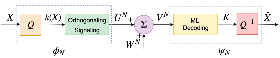
We will focus on schemes where the source $X$ is first quantized using $N$ levels and the quantization index $k(X)$ is mapped into orthogonal channel input vectors $U^{N}$ such that

thereby enforcing $||U^{N}||^{2}=E$. At the receiver, $k(X)$ is decoded using maximum likelihood (ML) estimation as $\hat{K}$, and the source is reconstructed as the $\hat{K}$th quantization level. Occasional decoding errors will be denoted by the outage event

This proposed coding scheme is illustrated as a block diagram in Fig. 1.

One convenient feature of ML estimation is that given the event ${\cal O}$, the reconstruction $\hat{X}$ is distributed uniformly over the incorrect reconstruction values of the quantizer. Also, it is not difficult to see that $X$ is independent of ${\cal O}$.

Using the outage notation, one can write the MSE as

In [2], it was shown that while keeping the outage event at a vanishingly small probability, i.e., $\Pr[{\cal O}]\leq\epsilon$ for arbitrary $\epsilon>0$, one can ensure that

as $\gamma\rightarrow\infty$. The significance of (5) is that it coincides with the best exponent theoretically achievable in the Shannon-theoretic scenario of encoding infinitely long source blocks at once.

In this work, we tackle (4) in its entirety and investigate the behavior of $-\ln\mathbb{E}[(X-\hat{X})^{2}]$ as a function of $\gamma$. No matter how small $\Pr[{\cal O}]$ is, it may affect the total expected distortion dramatically. More specifically, if it decays slower than $\mathbb{E}[(X\!-\!\hat{X})^{2}|\mathcal{O}^{c}]$ as $\gamma\rightarrow\infty$, it will dominate (4) and adversely affect the energy-distortion exponent.

In our analysis, we employ tools from high-resolution quantization theory. The high-resolution assumption is justified by the fact that the number of quantization levels $N$ must increase exponentially with $\gamma$ to ensure an exponentially decaying distortion, as will be apparent in the sequel. Distortion in the high-resolution regime is best understood with the help of companders [8] as shown in Fig. 2. First, a nonlinear compressor $G$ reduces the spread of large amplitudes and maps the source sample to $[0,1]$. Then, the source is uniformly quantized in the compressed domain with $N$ levels. Finally, a nonlinear expander $G^{-1}$ reverses this process by expanding the small amplitudes of uniformly quantized output. The end-to-end effect becomes a non-uniform quantizer. In fact, any non-uniform quantizer can be put into this form [8].

The point density function, $\lambda(x)=\frac{dG}{dx}$, provides one with an equivalent framework. It also has the convenient property that $\lambda(x)\geq 0$ and

That is, its behavior is the same as that of a probability density function (pdf).

It is well-known (cf. [9, 10]) that

where $D(N)$ denotes the MSE distortion incurred by an $N$-level quantizer, and $f(x)$ is the source pdf. The integral in (6) is known as the Bennett integral. We will use (6) to write

for any $\epsilon^{\prime}>0$ and large enough $N$.

We also have an upper bound on the outage probability

where we refer the reader to [2] and to the references therein for a detailed derivation of (8). We will use (6) and (8) in (4) to properly select $N$ such that the end-to-end distortion decays with the maximum possible speed.

Let $X\sim{\cal N}(0,1)$ and $N$ have the form of

where $c$ is a constant to be optimized and $\tau$ is to be picked later. Clearly, defining $N$ exponentially increasing in $\gamma$ is necessary to ensure that (6) decays exponentially in $\gamma$. Also observe that with this choice, even mediocre values of $\gamma$ will quickly drive $N$ to a very large number, thus justifying the high-resolution assumption.

Using (8), this choice yields

Similarly, using (7), we obtain

Therefore, according to (4), the remaining task is to understand how the term $\mathbb{E}[(X-\hat{X})^{2}|\mathcal{O}]$ behaves.

While in typical quantizer design problems the optimal $\lambda(x)$, i.e., minimizing (6), can be shown to be given by the well-known Panter-Dite formula, i.e.,

which, for the Gaussian source we consider, coincides with ${\cal N}(0,3)$, the current form of end-to-end distortion in (16) dictates a different solution. Writing the new problem formally, we have

It is easy to check that this is a convex optimization problem. One can therefore write an equivalent Lagrangian

and solve the optimization problem by seeking a solution to the Karush-Khun-Tucker (KKT) conditions

Taking the partial derivative above yields

Rewriting (17), we have

We attempt to find $\lambda(x)$ that satisfies KKT conditions for the case where $\alpha(x)=0$ and $\beta\geq 0.$ Thus, $\lambda(x)$ becomes

To satisfy the KKT conditions, it remains to pick $\beta$ such that $\lambda(x)$ integrates to $1$. Since (19) is decreasing in $\beta$, we can always find such a $\beta$ provided that $\int\lambda(x)dx\geq 1$ for $\beta=0$. Following this logic and substituting $\beta=0$ in (19), we observe that $c$ has to satisfy

or

For each $c\leq c_{0}$, denote by $\beta(c)$ the value of $\beta$ satisfying $\int\lambda(x)dx\geq 1$. For convenience, also set $\hat{\beta}(c)=\beta(c)e^{\gamma/6}$. The relationship between $c$ and $\hat{\beta}(c)$ is shown in Fig. 3.

Proceeding with (16),

Fig. 4 depicts $\Omega(c)$ as a function of $c$. The optimal values of $c$, $\hat{\beta}(c)$, and $\Omega(c)$ are numerically found to be $c_{opt}\approx 1.0327$, $\hat{\beta}_{opt}\approx 2.0771$, and $\Omega_{opt}\approx 9.6622$, respectively.

To analyze the characteristic of the distortion by means of higher order terms, let us rewrite (21) as

for large $\gamma$. Thus, for Gaussian sources, we obtained a lower bound to the dispersion, which is $\Upsilon(\gamma)\geq-2.2682$.

Fig. 5 shows the comparison between $\lambda(x)$ found and $\mathcal{N}(0,3)$, which would be the result of naïvely done quantization. It is not difficult to show that this choice (together with optimized $c$) would achieve a dispersion of $-2.3564$, and about $0.383$dB higher distortion for fixed $\gamma$. As can be observed from the figure, the new high-resolution quantizer has the point density function $\lambda(x)$ with a smaller variance (which is $1.93$) and it is no longer a Gaussian distribution.

For the aforementioned scenario, we also provide performance results for a uniform source, which is frequently studied in the literature. When $X\sim\mathcal{U}[-1/2,1/2]$, by following the same methodology, we derive the following upper bound:

Minimizing this bound, we obtain the optimal $\lambda(x)$ as

for $-1/2\leq x\leq 1/2$. By solving

in the same fashion as before, find $c_{0}=2.0801$, $\hat{\beta}_{opt}\approx 0.1385$, $c_{opt}\approx 0.8281$, and $\Omega_{opt}\approx 0.3884$. As a result, $-\ln D$ can be lower bounded as

Hence, the energy-distortion dispersion for a uniform source is lower bounded as $\Upsilon(\gamma)\geq 0.9458$.

Fig. 6 shows the comparison between the point-density functions $\lambda(x)$ of our approach and the naïve compander design, whcih would result in a uniformly distributed $\lambda(x)$. It is not difficult to show that the uniform $\lambda(x)$ would achieve an energy-distortion dispersion of $0.9242$, and about $0.0943$dB higher distortion for fixed $\gamma$.

In [6], an analytical upper bound for the distortion was derived using a linear quantizer and maximum a posteriori (MAP) receiver for a Gaussian source. Although their proposed scheme resulted in the same energy-distortion exponent under the asymptotic analysis, they disregarded the effect of the coefficient of the exponential term, causing a considerable performance degradation in the distortion, as we show next. By following the approach in [6], $D$ is calculated as follows.

where $\rho$ is a constant between $[0,1]$, $\Delta=2\sqrt{b\ln 2}$ and $b\geq 2$ is an integer representing the quantization bits per source component. For large enough $b$, $\frac{1}{(2^{b}-2)^{2}}$ can be approximated by $2^{-2b}$, and $D$ becomes

In [6], since the truncation was applied to a Gaussian source and it was quantized by using a uniform scalar quantizer, overload distortion was no longer negligible in terms of energy-distortion tradeoff. In [11], it was shown that overall distortion for a Gaussian density under uniform quantization decreases as $\frac{\ln N}{N^{2}}$ and overload distortion becomes asymptotically negligible. However, this causes the energy-distortion dispersion to diverge when there is a zero-delay constraint and $\gamma\rightarrow\infty$.

As an alternative to the analytical solution, we also provide a numerical solution to this problem by finding optimal values of $\rho$ and $b$ that minimize (25) for each value of $\gamma$. Comparison of the distortions of our approach, approaches in [2], [6] is illustrated in Fig. 7. The blue curve indicates the result of the distortion that is suggested in this work, in which $\lambda(x)$ is optimized, while the magenta curve shows the distortion for the case where $\lambda(x)=\mathcal{N}(0,3)$. The green curve depicts the numerical optimization of the distortion in [6], whereas the yellow curve shows the analytical result of the asymptotic distortion in that work. We note that the distortion gap between our approach and that of [6] diverges as $\gamma$ grows without bound.

References

- [1] R. R. Mohassel, A. S. Fung, F. Mohammadi, and K. Raahemifar, “A survey on advanced metering infrastructure and its application in smart grids,” in 2014 IEEE 27th Canadian Conference on Electrical and Computer Engineering (CCECE), May 2014, pp. 1–8.
- [2] E. Koken, D. Gunduz, and E. Tuncel, “Energy-distortion exponents in lossy transmission of Gaussian sources over Gaussian channels,” IEEE Transactions on Information Theory, vol. 63, no. 2, pp. 1227–1236, Feb 2017.
- [3] V. Kostina and S. Verdu, “Fixed-length lossy compression in the finite blocklength regime,” IEEE Transactions on Information Theory, vol. 58, no. 6, pp. 3309–3338, June 2012.
- [4] Y. Polyanskiy, H. V. Poor, and S. Verdu, “Channel coding rate in the finite blocklength regime,” IEEE Transactions on Information Theory, vol. 56, no. 5, pp. 2307–2359, May 2010.
- [5] M. Burnashev, “On minimum attainable mean-square error in transmission of a parameter over a channel with white Gaussian noise,” Problems Inform. Transmission, vol. 21, no. 4, pp. 247–257, 1985.
- [6] F. A. Abdallah and R. Knopp, “Source-channel coding for very-low bandwidth sources,” in 2008 IEEE Information Theory Workshop, May 2008, pp. 184–188.
- [7] N. Merhav, “On optimum parameter modulation-estimation from a large deviations perspective,” IEEE Transactions on Information Theory, vol. 58, no. 12, pp. 7215–7225, Dec 2012.
- [8] A. Gersho and R. M. Gray, Vector Quantization and Signal Compression. Norwell, MA, USA: Kluwer Academic Publishers, 1991.
- [9] P. Zador, “Development and evaluation of procedures for quantizing multivariate distributions,” Ph.D. dissertation, Stanford University, 1963.
- [10] A. Gersho, “Asymptotically optimal block quantization,” IEEE Transactions on Information Theory, vol. 25, no. 4, pp. 373–380, July 1979.
- [11] D. Hui and D. L. Neuhoff, “Asymptotic analysis of optimal fixed-rate uniform scalar quantization,” IEEE Transactions on Information Theory, vol. 47, no. 3, pp. 957–977, Mar 2001.