Coherent double coverings of virtual link diagramsThanks: This work was supported by JSPS KAKENHI Grant Number 15K04879.
Abstract.
A virtual link diagram is called normal if the associated abstract link diagram is checkerboard colorable, and a virtual link is normal if it has a normal diagram as a representative. Normal virtual links have some properties similar to classical links. In this paper, we introduce a method of converting a virtual link diagram to a normal virtual link diagram. We show that the normal virtual link diagrams obtained by this method from two equivalent virtual link diagrams are equivalent. We discuss the relationship between this method and some invariants of virtual links.
1. Introduction
Virtual links correspond to stable equivalence classes of links in thickened surfaces [1, 5]. A virtual link diagram is called normal if the associated abstract link diagram is checkerboard colorable ( 2). A virtual link is called normal or checkerboard colorable if it has a normal diagram as a representative. Every classical link diagram is normal, and hence the set of classical link diagrams is a subset of that of normal virtual link diagrams. The set of normal virtual link diagrams is a subset of that of virtual link diagrams. Jones polynomial is extend to virtual links [7]. It is shown in [3] that Jones polynomial of a normal virtual link has a property that Jones polynomial of a classical link has. For this property Khovanov homology is extended to normal virtual links in a natural way as stated in O. Viro [10]. The author introduced the method of converting a virtual link diagram to a normal virtual link diagram by use of the double covering technique in [4]. In this method, two converting virtual link diagrams obtained from two equivalent virtual link diagrams are related by generalized Riedemeister moves and K-flypes (See [4]).
In this paper, we introduce another method of converting a virtual link diagram to a normal virtual link diagram, which is called the coherent double covering technique. We show that two normal virtual link diagrams obtained from two equivalent virtual link diagrams by our method are equivalent as a virtual link. In Section 4, we discuss the relationship between our method and some invariants of virtual links, as the odd writhe, the invariant of even ordered virtual link which is introduced by H. Miyazawa, K. Wada and Y. Yasuhara[9].
2. Definitions and main results
A virtual link diagram is a generically immersed, closed and oriented 1-manifold in with information of positive, negative or virtual crossing, on each double point. A virtual crossing is an encircled double point without over-under information [7]. A virtual link is an equivalence class of virtual link diagrams under Reidemeister moves and virtual Reidemeister moves depicted in Figure 1. We call Reidemeister moves and virtual Reidemeister moves generalized Reidemeister moves.
I II III Reidemeister moves
I II III IV Virtual Reidemeister moves
An abstract link diagram (ALD) is a pair of a compact surface and a link diagram on such that the underlying 4-valent graph is a deformation retract of .
We obtain an ALD from a virtual link diagram by corresponding a diagram to an ALD as in Figure 2 (i) and (ii). Such an ALD is called the ALD associated with . Figure 3 shows a virtual link diagram and the ALD associated with it. For details on abstract link diagrams and their relations to virtual links, refer to [5].
(i) (ii) (iii)

 (i)
(ii)
(i)
(ii)
Let be a virtual link diagram and the ALD associated with . The diagram is said to be normal or checkerboard colorable if the regions of can be colored black and white such that colors of two adjacent regions are different. In Figure 4, we show an example of a normal diagram. (The orientations of the diagrams in Figure 4 are alternate orientations, which are discussed later.) A classical link diagram is normal. A virtual link is said to be normal if it has a normal virtual link diagram. Note that normality is not necessary to be preserved under generalized Reidemeister moves. For example the virtual link diagram in the right of Figure 5 is not normal and is equivalent to the trefoil knot diagram in the left which is normal.


H. Dye introduced the notion of cut points on a virtual link diagram in [2].
Let be a pair of a virtual link diagram and a finite set of points on edges of . We obtain an ALD from as in Figure 2 (i), (ii) and (iii) and call it the ALD associated with . See Figure 6 (ii) and (iii). If the ALD associated with is normal, then we call the set of points a cut system of and call each point of a cut point. For the virtual link diagram in Figure 6 (i) we show an example of a cut system in Figure 6 (ii) and the ALD associated with it with a checkerboard coloring in Figure 6 (iii).

A virtual link diagram is said to admit an alternate orientation if it can be given an orientation such that an orientation of an edge switches at each classical crossing as in Figure 7. (Here an edge means an edge of , where endpoints are classical crossings and there might be some virtual crossings on it.) The virtual link diagram in Figure 4 admits an alternate orientation. It is known that a virtual link diagram is normal if and only if it admits an alternate orientation [6].

Note that a finite set of points on is a cut system if and only if admits an alternate orientation such that the orientations of edges are as in Figure 7 at each classical crossing of and each point of (cf. [4, 6]).
The canonical cut system of a virtual link diagram is the set of points that is obtained by giving two points in a neighborhood of each virtual crossing of as in Figure 8 (i).

Proposition 1 ([4]).
The canonical cut system is a cut system.
Dye introduced cut point moves depicted in Figure 9. Then we have the following.
I II III
Theorem 2 ([4]).
For a virtual link diagram , two cut systems of are related by a sequence of cut point moves I, II and III.
Corollary 3 ([2], c.f. [4]).
For any virtual link diagram with a cut system, the number of cut points is even.
Let be a virtual link diagram with a cut system . Assume that is on the right of the -axis in the -plane and all crossings and cut points have distinct -coordinates. Let be a copy of on the left of the -axis in the -plane which is obtained from by sliding along the -axis. Let be the set of cut points of and for , we denote by the cut point of corresponding to . See Figure 10 (i).


(i) (ii)
For horizontal lines such that contains and the corresponding cut point of , we replace each part of in a neighborhood of for each as in Figure 11. We denote by the virtual link diagram obtained this way.
For example, for the virtual link diagram with the cut system depicted as in Figure 10 (i), the virtual link diagram is as in Figure 10 (ii).

Then we have the following.
Proposition 4.
For a virtual link diagram with a cut system , , is normal.
Proof.

Then we have
Remark 5.
Precisely speaking, is well-defined when satisfies that all crossings and cut points have distinct -coordinates. If we change by an isotopy of , is preserved under an isotopy of and virtual Reidemeister moves.
Let be a virtual link diagram with a cut system . We call the converted normal diagram or the coherent double covering diagram of . Let be a virtual link diagram. For the canonical cut system of , we denote by the converted normal diagram . We call the canonical converted normal diagram of . Then we have
The following is our main theorem.
Theorem 6.
Let and be virtual link diagrams with cut systems. If and are equivalent, then the converted normal diagrams and are equivalent. In particular, if and are equivalent, then the canonical converted normal diagrams and are equivalent.
3. Proof of Theorem 6
Lemma 7.
Let be a virtual link diagram. Suppose that and are cut systems of . Then the converted normal diagrams and are equivalent.
Proof.

 (i)
(ii)
(i)
(ii)

(iii)
Lemma 8.
Let and be virtual link diagrams. If and are equivalent then the canonical converted normal virtual link diagrams and are equivalent.
Proof.
Let be a virtual link diagram with the canonical cut system . Suppose that a virtual link diagram is obtained from by one of generalized Reidemeister moves and is the canonical cut system of . If is related to by one of Reidemeister moves, then and are related by two Reidemeister moves. As in Figure 14 (i) (or (ii)), suppose that is related to by a virtual Reidemeister move I (or II) and let be the cut system obtained from by cut point moves I and II as in the figure. By Lemme 7, and are equivalent. On the other hand and are related by two virtual Reidemeidter moves I (or II) as in Figure 14 (i) (or (ii)). Thus and are equivalent. As in Figure 14 (iii), suppose that is related to by a virtual Reidemeister move III and let (or ) be the cut system obtained from (or ) by cut point moves I and II as in the figure. By Lemme 7, (or ) and (or ) are equivalent. On the other hand, and are related by two virtual Reidemeidter move III. As in Figure 14 (iv), suppose that is related to by a virtual Reidemeister move IV and let (or ) be the cut system obtained from (or ) by cut point moves I and II (or cut point moves I , II and III) as in the figure. By Lemme 7, (or ) and (or ) are equivalent. On the other hand, as in Figure 14 (v), and are equivalent by virtual Reidemeister moves.
In Figure 14, if the orientation of some strings of virtual link diagram are different from those of it, we have the result by a similar argument.
 |
 |
 |
| Virtual Reidemeister move I | Virtual Reidemeister move II | Virtual Reidemeister move III |
| (i) | (ii) | (iii) |
 |
 |
| Virtual Reidemeister move IV | Coherent double covering diagrams (virtual Reidemeister move IV) |
| (iv) | (v) |
4. A relationship between invariants and coherent double covering diagrams
In this section we discuss a relationship between some invariants and coherent covering diagrams.
4.1. Odd writhe
We give an interpretation of the odd writhe of a virtual knot in terms of the linking number of the converted normal diagram . The argument of this subsection is similar to that of Section 4 in [4].
For a 2-component virtual link diagram , the half of the sum of signs of nonself classical crossings of is called the linking number of . The linking number is an invariant of 2-component virtual link.
Theorem 9.
Let be a virtual knot diagram with a cut system. Then is a 2-component virtual link diagram and the linking number of is an invariant of the virtual knot represented by .
The odd writhe is a numerical invariant of virtual knots [8]. We recall the definition of the odd writhe later.
Theorem 10.
Let be a virtual knot diagram with a cut system. The linking number of is equal to the odd writhe of .
Let be a virtual link diagram. The Gauss diagram of is a set of oriented circles which are the preimage of with oriented chords each of which corresponds to a classical crossing and its tail (or its head) indicates an overpass (or an underpass) of the classical crossing. Each chord is equipped with a sign of the corresponding classical crossing. The Gauss diagram in Figure 15 (i) is that of the virtual knot diagram in Figure 3 (i).

For a virtual link diagram with a cut system , the Gauss diagram with points, denoted by , of is obtained from the Gauss diagram of by adding points on arcs which correspond to the points of . We denote by the Gauss diagram of and by the points of corresponding to . Then . In Figure 15 (ii) we show the Gauss diagram with points of the virtual link diagram with points in Figure 6 (ii). Let be the virtual link diagram with a cut system which is a copy of . The Gauss diagram with points is a copy of . The Gauss diagram of is obtained from the Gauss diagrams of by a local replacement around each point of the Gauss diagram and around the corresponding point of as in Figure 16. For a virtual knot diagram of with a set of points on edges , we denote the Gauss diagram of by . The Gauss diagram in Figure 15 (iii) is for depicted in Figure 6 (ii) by the map .

For the Gauss diagram of , , suppose that are points in such that the point follows the point along the orientation of and the point in corresponds to the point . In what follows, we denote by the same symbol (or ) for the point of (or of ) and the corresponding point of (or ).
Let (or ) be the arc of the Gauss diagram of between two points and (or and ), and the arc between two points and (or and ) is (or ). Note that corresponds to . We also denote an arc of which corresponds to or of by or , respectively. Here (or ) is the arc in which is obtained from (or ) by removing a regular neighborhood of and (or and ).
Lemma 11.
Let be a virtual knot diagram with points . Suppose for a positive integer . Then is a 2-component virtual link diagram . Furthermore if an arc is in (or ), then and are in (or ).
Proof.
We use the induction on . Suppose that , i.e. is a virtual knot diagram with 2 points and . The Gauss diagram is depicted as in Figure 17, where the bold line and the thin line indicate the different components and we dropped all chords in the figure. In this case is a 2-component virtual link diagram. Two arcs and are in one component of , and and are in the other.
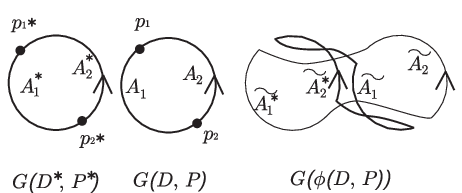
Suppose that the statement is hold if the number of points is less than . We assume that is a virtual knot diagram with points . First, apply the replacement as in Figure 16 to points and . Then we obtain a Gauss diagram with points and . By the hypothesis, the Gauss diagram is depicted as in Figure 18 (i), where two arcs and (or two points and ) are in one component of and two arcs and (or two points and ) are in the other. If an arc is in one component of , (or ) is in the other for by the induction hypothesis. By applying the replacement in Figure 16 to two pairs of points and and and of the Gauss diagram , we have a Gauss diagram as in Figure 18 (ii). Therefore we have the result.

Proof of Theorem 9.
For a virtual knot and its diagram with the cut system , we denote the linking number of by or . Theorem 10 states that is equal to the odd writhe of .
Let be a virtual knot diagram and be a Gauss diagram of . For a classical crossing , we denote by the chord of corresponding to . The endpoints of divides the circle of into 2 arcs. We denote the arcs by and where is the arc which starts from the tail of and terminates at the head. A classical crossing of is said to be odd if there are an odd number of endpoints of chords of on . The odd writhe of is the sum of signs of odd crossings of .Note that if a virtual knot diagram is normal, all classical crossings are not odd and hence the odd writhe is zero.
It is shown in [8] that the odd writhe is an invariant of virtual knots.
Proof of Theorem 10.
Let be a virtual knot diagram and be a cut system of . It is sufficient to show that odd crossings of correspond to nonself classical crossings of . Since admits an alternate orientation, the circle of the Gauss diagram of admits an alternate orientation such that one endpoint of each chord is a sink of the orientations and the other is a source. This implies the following condition:
- ()
For any classical crossing of , the sum of the number of cut points on the arc and that of endpoints of chords appearing on , is even.
Let be the arcs obtained by cutting the circle of along the cut points. We assume that the arc appears after the arc along the orientation of . We also denote by the arc of which corresponds to . For a classical crossing of , the classical crossing corresponding to in is denoted by . Let be an odd crossing of . Suppose that one endpoint of is on and the other endpoint is on . By definition, there are an odd number of endpoints of chords on in . By the condition () above, we see that there are an odd number of cut points on in . Then we see that is not congruent to modulo . By Lemma 11 and in are in distinct components of . Thus the classical crossing is a nonself classical crossing of . By a similar argument, we see that if is not an odd crossing of , then is a self classical crossing of .
We show some properties of . They are also obtained from the properties of the odd writhe.
Corollary 12 ([8]).
Let be a normal virtual knot. Then is zero.
Proof.
Let be a normal knot diagram of . The empty set is a cut system. The virtual link diagram is the disjoint union, of and . Thus is zero.
Let be a virtual knot diagram. The virtual knot diagram obtained from by switching the over-under information of all classical crossing (or by reflection) is denoted by (or ).
Corollary 13 ([8]).
Let be a virtual knot diagram. If is not zero, then is not equivalent to (or .
Proof.
It is clear that . This implies the result.
For example, the virtual knot presented by the diagram in Figure 19, is not normal by Corollary 12, since . By Corollary 13, is not equivalent to (or .

4.2. Linking invariants of even virtual links
H. Miyazawa K. Wada and A. Yasuhara defined an invariant of even virtual links by use of the virtual orientation. We give another definition of their invariant.
Let be a virtual link diagram. is said to be even, if on each circle of a Gauss diagram of there is an even number of endpoints of chords. A virtual knot diagram is even. If a virtual link diagram is even, any virtual link diagram which is equivalent to is even. Note that when we go around each component of an even virtual link diagram, we meet an even number of virtual crossings. A normal virtual link diagram is even, and any a virtual link diagram which presents a normal virtual link is even.
Let be an ordered unoriented even -component virtual link diagram such that where is a component of . The virtual orientation is an orientation of such that they switch an opposite direction at each virtual crossing of as in Figure 20. (The orientation is not switched at classical crossings.)

We give a virtual orientation . The sum of signs of classical crossings between and whose overpass of is denoted by under the virtual orientation .
Theorem 14 ([9]).
is an invariant of ordered unoriented even virtual links.
Proposition 15.
The number of cut points of each component of an even virtual link diagram with a cut system is even.
Proof.
Let be even virtual link diagram with the canonical cut system . Each component of has an even number of cut points, since we meet an even number virtual crossings when we go around each component of it. Any cut system of is obtained from by cut point moves I, II and III. Then we have the same result in another cut system of since by a cut point move II or III changes the number of cut points on a component of by or .
Let be an even -component virtual link diagram such that where is a component of . Suppose that is a cut system of . A cut orientation is an orientation of such that they switch an opposite direction at each cut point of as in Figure 21. We denote it . (For a cut orientation, the orientation is not switched at classical crossings and virtual crossings.)

Let be even virtual link diagram with a cut system such that where is a component of . We give a cut orientation . The sum of signs of classical crossings between and whose overpass of is denoted by under the cut orientation .
Proposition 16.
For two cut systems and of , let (or ) be a cut orientation of (or ). Then we have .
Proof.
Suppose that is obtained form by one of cut point moves I, II and III to a component (or two components and ) of as in Figure 22 (i), (ii) (or (iii)). The cases of a cut point moves I (or II), we give a cut orientation to as in Figure 22 (i) (or (ii)) and to as in Figure 22 (i) (or (ii)) (a) or (b). In both cases, if a sign of each classical crossing between and of with respect to is , the sign of with respect to is . The case of a cut point moves III, we give a cut orientation to as in Figure 22 (iii) and to as in Figure 22 (iii) (a), (b), (c) or (d). In each case, if a sign of each classical crossing between and of with respect to is , the sign of with respect to is . Thus we have the result.

We denote by .
Theorem 17.
coincides to . Thus is an invariant of ordered unoriented virtual link.
Proof.
Let be an ordered unoriented even -component virtual link diagram such that where is a component of . We give a virtual orientation of , to . Let be the canonical cut system of . There is a cut orientation of whose orientation of each arc of corresponds to that of in as in Figure 23.

We give an interpretation of the linking invariant in terms of our covering method. Let be an even -component virtual link diagram with a cut system such that where is a component of . We give an cut orientation to . Let be a copy of and be the cut orientation of such that an orientation of each arc of is different from the corresponding arc of in . We take the coherent double covering diagram of in the same manner as in Figure 11. We call this the coherent double covering diagram with a cut orientation denoted by . The virtual link diagram in Figure 24 (ii) is the coherent double covering diagram of the virtual link diagram in Figure 24 (i) with a cut orientation . Note that the orientation of the coherent double covering diagram derived from cut orientations and .


(i) (ii)
Let be an ordered unoriented even -component virtual link diagram with a cut system such that where is a component of . We denote the subset of the cut system whose points are on arcs of by . A component of the Gauss diagram of corresponding a component with by . For the Gauss diagram of , , suppose that (or ) are points in such that the point follows the point along and the point in coressponds to the point . In what follows, we denote by the same symbol (or ) for the point of (or of ) and the corresponding point of (or ).
Let (or ) be the arc of the Gauss diagram of between two points and (or and ), and the arc between two points and (or and ) is (or ). Note that corresponds to . We also denote an arc of which corresponds to (or ) of by (or ), respectively.
Lemma 18.
Let be an even -component virtual link diagram with a cut system such that where is a component of . Then is a 2-component virtual link diagram such that is a 2-component link diagram . Furthermore if an arc is in (or ), then and are in (or ).
Proof.
The proof is obtained by a similar argument as in Lemma 11.
Let be an ordered unoriented even -component virtual link diagram with a cut system such that where is a component of . We denote the subset of the cut system whose points are on arcs of by . For a classical crossing between and of , the classical crossing corresponding to in between and is denoted by ().
Let between and of such that an arc of is an overpass of . Then the overpass of a classical crossing in corresponding , is in . For the other classical crossing corresponding , its overpass is in where and by Lemma 18. Then we have the following theorem.
Theorem 19.
Let be an ordered unoriented even -component ordered unoriented virtual link diagram with a cut system such that where is a component of . For a cut orientation of , the absolute value of the sum of the classical crossings between and whose overpasses are in in the coherent double covering diagram with a cut orientation of , coincides to .
Proof.
Let be a classical crossing of between and whose overpass is in . One of two classical crossings of corresponding to is between and , and its overpass is in . The sign of such a classical crossing is equal to that of .
For an ordered unoriented even virtual link diagram with a virtual orientation in Figure 25 (i), . In Figure 25 (ii), the diagram D with a cut system and a cut orientation and an coherent double covering diagram of with a cut orientation , are depicted, where correspond to a component of . The absolute value of the sum of the classical crossings between (or ) and whose overpasses belong to (or ) coincides to for .

Let be an ordered oriented even -component virtual link diagram with a cut system such that where is a component of . For a cut system of , we denote a -component sub-diagram of the coherent double covering diagram which corresponds to , by . Let be the linking number between and for .
The set is denoted by (). For a virtual knot diagram , is , where .
Corollary 20.
The set is an invariant of ordered oriented even virtual links. Furthermore is equal to the set and , . The linking number is an invariant of an ordered oriented even virtual link.
Proof.
Let be an ordered oriented even -component virtual link diagram with a cut system such that where is a component of . Let be a classical crossing between and of . If one calssical crossing in corresponding is between and and, then the other is a classical crossing between and for and . The sings of two classical crossings and are the same. Then we have and .
Let an ordered oriented even virtual link diagrams with a cut system () and with a cut system be as in Figure 26 (i). In Figure 26 (ii) we show a coherent double covering diagram . We have and . So is not equivalent to .

Acknowledgement
The author would like to thank Seiichi Kamada for his useful suggestion.
References
- [1] J. S. Carter, S. Kamada and M. Saito, Stable equivalence of knots on surfaces and virtual knot cobordisms, J. Knot Theory Ramifications 11 (2002) 311–322.
- [2] H. Dye An invitation to knot theory, CRC Press, 2016.
- [3] N. Kamada, On the Jones polynomials of checkerboard colorable virtual knots, Osaka J Math., 39 (2002), 325–333.
- [4] N. Kamada, Converting virtual link diagrams to normal ones, Topology and its Applications, to appear. DOI: 10.1016/j.topol.2017.08.032
- [5] N. Kamada and S. Kamada, Abstract link diagrams and virtual knots, J. Knot Theory Ramifications 9 (2000) 93-106.
- [6] N. Kamada, S. Nakabo and S. Satoh, A virtualized skein relation for Jones polynomials, Illinois J. Math. 46 (2002), 467–475.
- [7] L. H. Kauffman, Virtual knot theory, European J. Combin. 20 (1999) 663–690.
- [8] L. H. Kauffman, A self-linking invariant of virtual knots. Fund. Math., 184 (2004), 135–158.
- [9] H. Miyazawa, K. Wada, A. Yasuhara Linking invariants of even virtual links, preprint.
- [10] O. Viro, Virtual Links, Orientations of Chord Diagrams and Khovanov Homology, Proceedings of 12th Gökova Geometry-Topology Conference, (2007) 184–209.