Weak Mixing Angle in the Thomson Limit

The electroweak sector of the Standard Model is based on the gauge symmetry group $SU\left(2\right)_{L}\times U\left(1\right)_{Y}$. The weak mixing angle, $\theta_{W}$, is a parameter that describes the mixing of the gauge bosons related to the $U\left(1\right)_{Y}$ and the third component of $SU\left(2\right)_{L}$ to give rise to the mass eigenstates of the photon and the $Z$ boson. In terms of the couplings $g$ of $SU\left(2\right)_{L}$ and $g^{\prime}$ of $U(1)_{Y}$ one has

Since it is given explicitly by gauge couplings, $\sin^{2}\hat{\theta}_{W}$ depends on the energy scale and is governed by a renormalization group equation (RGE) [1, 2].

One of the tests of the Standard Model is to evolve the weak mixing angle from high to low energies and compare it with experimental extractions at lower squared momentum transfers, $Q^{2}$. For example, the Qweak experiment [3] at Jefferson Laboratory (JLab) has measured the weak charge of the proton, $Q_{W}(p)\sim 1-4\sin^{2}\theta_{W}$, in polarized electron scattering from a fixed liquid hydrogen target at $Q^{2}\approx 0.026$ GeV². The same observable, but at an even lower $Q^{2}\approx 0.0045$ GeV², will also be targeted by the P2 experiment [4] at the MESA facility which is currently under construction at the University of Mainz in Germany. In a very similar setup, the MOLLER Collaboration [5] at JLab will build and improve on the completed E158 experiment [6] at SLAC (that occurred at almost the same $Q^{2}$ as Qweak) and measure the analogous weak charge of the electron, $Q_{W}(e)$, in polarized Møller scattering at $Q^{2}\approx 0.0056$ GeV². The PVDIS Collaboration [7] at the 6 GeV CEBAF complex at JLab scattered polarized electrons deep-inelastically from deuterium, and the SoLID Collaboration [8] will increase the PVDIS precision in the future by benefiting from the energy upgraded CEBAF and a correspondingly higher and broader $Q^{2}$ range. Other approaches include neutrino and anti-neutrino deep inelastic scattering [9], $\bar{\nu}$-$e$ scattering near nuclear reactors [10], and parity violation in atoms [11] and ions [12]. For more details, see the recent reviews on low energy measurements of the weak mixing angle [13], on the weak neutral current [14], and on weak polarized electron scattering [15].

Since QCD at low energies does not allow for reliable perturbative calculations, the theoretical uncertainty of the RGE running from the $Z$-pole to low energies arises dominantly from the hadronic region. A phenomenological approach to address this region was developed in Ref. [2]. Working in the $\overline{\mbox{\small MS}}$ scheme¹¹ 1 Quantities defined in the $\overline{\mbox{\small MS}}$ scheme will be denoted by a caret., the main idea was to relate the case of the weak mixing angle to that of the electromagnetic coupling, $\hat{\alpha}$, as far as possible, and then to consider both maximal and minimal $SU(3)$ flavor symmetry breaking to constrain the flavor separation of the three light quarks $(u,d,s)$. In the present work, we extend the analysis to the next order in the strong coupling constant, $\hat{\alpha}_{s}$, and introduce a number of new elements. We employ the most recent values and uncertainties of the input parameters, such as $\hat{\alpha}_{s}$ and the heavy quark masses. The hadronic vacuum polarization contribution to the RGE running of $\hat{\alpha}$ is obtained dispersively from $e^{+}e^{-}$ annihilation data for hadronic final states, which are supplemented by isospin rotated $\tau$ decay spectral functions corrected for isospin breaking effects [16, 17]. We tie experimental data [16] and lattice gauge theory calculations [18, 19] together to obtain the individual contributions of strange and first generation quarks. This flavor separation at the quark level to high accuracy is consistent with and almost an order of magnitude more precise than previous calculations [1, 2]. It is also necessary to constrain OZI-rule [20, 21, 22] violating effects, for which we utilize the recent lattice gauge theory calculation of disconnected contributions to the anomalous magnetic moment of the muon [23]. These refinements allow for significant reduction of the theoretical uncertainty of the RGE evolution. As a by-product, our method sheds light on the dual description of quarks and hadrons in the non-perturbative regime and may open new ways to extract the strange quark mass from the electro-production of hadrons.

The paper is organized as follows: Section 2 presents the RGE of the weak mixing angle up to five loop accuracy, and the matching conditions for $\hat{\alpha}$ and $\sin^{2}\theta_{W}$. In Section 3 we perform the conversion of the hadronic vacuum polarization contribution to the running of $\hat{\alpha}$ from the on-shell scheme, where it is most directly obtained, to the $\overline{\mbox{\small MS}}$ scheme (Appendix A contains a brief discussion of various calculations of $\alpha(M_{Z})$). Section 4 describes the calculation of the singlet contribution to the weak mixing angle, with some details given in Appendix B. In Section 5 the flavor separation (contributions of light and strange quarks) is addressed and threshold masses are calculated. In Section 6 theoretical uncertainties are discussed in detail, and Section 7 offers our final results and conclusions.

In an approximation in which all fermions are either massless and active or infinitely heavy and decoupled, the RGE for the electromagnetic coupling in the $\overline{\mbox{\small MS}}$ scheme [24], $\hat{\alpha}$, can be written in the form [2],

where the sum is over all active particles in the relevant energy range. The $Q_{i}$ are the electric charges, while the $\gamma_{i}$ are constants depending on the field type and shown in Table 1.

The $K_{i}$ and $\sigma$ contain higher-order corrections and are given by [25],

and,

with $n_{q}$ the number of active quarks and $N_{i}^{c}=3$ the color factor for quarks. For leptons one substitutes $N_{i}^{c}=1$ and $\hat{\alpha}_{s}=0$, while $K_{i}=1$ for bosons.

We can relate the RGE of $\hat{\alpha}$ to that of $\sin^{2}\hat{\theta}_{W}$ since both, the $\gamma Z$ mixing tensor $\hat{\Pi}_{\gamma Z}$ and the photon vacuum polarization function $\hat{\Pi}_{\gamma\gamma}$ are pure vector-current correlators. Including higher order corrections, the RGE for the $Z$ boson vector coupling to fermion $f$, $\hat{v}_{f}=T_{f}-2Q_{f}\sin^{2}\hat{\theta}_{W}$, where $T_{f}$ is the third component of weak isospin of fermion $f$, is then

Eqs. (2) and (5) can be used [2] to obtain

where the $\lambda_{i}$ are known [2] constants given in Table 2 and the explicit $K_{i}$ dependence has disappeared. The $\tilde{\sigma}$ terms,

with,

represent the singlet contributions to the RGE evolution of the weak mixing angle at four and five loop order. These terms arise from quark-antiquark annihilation (disconnected) diagrams (see Figure 1) and are suppressed in perturbative QCD (PQCD). In the non-perturbative domain these give rise to so-called OZI-rule [20, 21, 22] violations.

Eq. (6) together with the solution of the four-loop QCD $\beta$-function [26, 27] represents a complete solution, as long as all matching scales $\mu$ at which an active particle decouples are known, because there the $\lambda_{i}$ change their values. The matching scales of all bosons [28], charged leptons, and heavy ($t$, $b$, and $c$) quarks [29, 30, 31] can be calculated as what we call threshold masses $\bar{m}_{q}$, where the QCD corrections to the matching relations vanish by definition.

The perturbative treatment of the previous section cannot be applied at hadronic energy scales and experimental input is required. This is usually taken from $R(s)$, i.e., the cross section $\sigma(e^{+}e^{-}\to\mbox{ hadrons})$ normalized to $\sigma(e^{+}e^{-}\to\mu^{+}\mu^{-})$. Additional information on $R(s)$ is encoded in hadronic $\tau$ decay spectral functions [32]. The traditional method to implement the $R(s)$ measurements is through a subtracted dispersion integral,

which gives the hadronic contribution (with the top quark removed) to the $Z$ scale value of the electromagnetic coupling in the on-shell scheme. One supplements the input data with the theoretical (perturbative) prediction for $R(s)$ at $s\geq s_{0}$, with $s_{0}$ large enough to be able to trust QCD perturbation theory. A variant [33] of this approach evaluates Eq. (13) in the space-like region, $\Delta\alpha^{(5)}_{\rm had.}(-M_{Z}^{2})$, and obtains $\Delta\alpha^{(5)}_{\rm had.}(M_{Z}^{2})$ in a second step. More details about how different groups get the running of alpha are given in Appendix A.

In the $\overline{\mbox{\small MS}}$ scheme it is more natural to use an unsubstracted dispersion relation [24],

where the superscript indicates that we focus here on the currents produced by the three light quarks (bosons, leptons, charm and bottom quarks are included following Sec. 2). The upper integration limit can in principle be chosen as an arbitrary perturbative scale $\mu_{0}$, but in practice we take $\mu_{0}^{2}$ to coincide with the cut-off value $s_{0}$ used in the traditional method, since this allows us to recycle results obtained there. Indeed [24],

for $\mu_{0}\lesssim 2$ GeV. Using the results of Ref. [16] including inputs from $\tau$ decays which we correct for $\gamma$-$\rho$ mixing [17], we obtain,

We compute the second term in Eq. (14) at the scale $\mu=2$ GeV perturbatively [34], extending the ${\mathscr{O}}(\hat{\alpha}_{s}^{2})$ result of Ref. [24] to ${\mathscr{O}}(\hat{\alpha}_{s}^{3})$,

where the $F_{i}(\hat{m}_{c},\hat{m}_{b})$ are correction terms from the charm and bottom quarks. The explicit analytical expression for ${F_{2}(\hat{m}_{c},\hat{m}_{b})\simeq-0.2348}$ is given in Ref. [24], while that for $F_{3}(\hat{m}_{c},\hat{m}_{b})\simeq-0.390$ will appear in ref. [34]. The numerical evaluation in the last line of Eq. (17) is for $\hat{\alpha}_{s}(M_{Z})=0.1182$, $\hat{\alpha}_{s}(2~\text{GeV})=0.303$ and $\hat{m}_{s}(2~\mbox{GeV})=98\pm 6$ MeV [35]. The uncertainty is the size of the ${\mathscr{O}}(\hat{\alpha}_{s}^{3})$ term, and we have defined

to display the dependence on $\hat{\alpha}_{s}$. Thus, from Eqs. (14)–(17) we obtain,

We recall that Eq. (7) exhibits an explicit dependence on $\alpha_{s}$, which in the non-perturbative domain gives rise to the QCD induced OZI-rule [20, 21, 22] violations. These have to be known independently, since they affect $\hat{\alpha}$ and $\hat{s}^{2}$ differently. Thus, in addition to a quark flavor separation, one also needs a singlet piece separation, even though the singlet piece is expected to be small. To do so, we first relate $\Delta_{\rm disc}\hat{\alpha}$, the disconnected part in $\Delta\hat{\alpha}^{(3)}(2\mbox{ GeV})$, to the one entering the low energy weak mixing angle, $\Delta_{\rm disc}\hat{s}^{2}$. Non-singlet and singlet contributions are separately gauge-invariant, and to gain information on $\Delta_{\rm disc}\hat{\alpha}$, we will adopt a lattice QCD calculation [23] of the disconnected quark line contributions to the anomalous magnetic moment of the muon, $a_{\mu}$.

By construction, the $\tilde{\sigma}$ terms in Eq. (6) are related to the $\sigma$ terms in Eq. (2),

On the other hand, isolating the $\Delta_{\rm disc}\hat{\alpha}$ term in Eq. (2) we obtain (working here in lowest order in $\alpha$),

so that,

where the last step applies for $\mu<\bar{m}_{c}$ (we are assuming approximate isospin symmetry which eliminates the interval $\bar{m}_{u}<\mu<\bar{m}_{d}$). Then,

These relations are general, but there is a subtle point. In general, the singlet pieces effectively decouple at renormalization scales $\bar{m}^{\rm disc}_{q}$ that may differ from the scales $\bar{m}_{q}$ at which the non-singlet pieces decouple. This would generate various energy intervals with generally different values for $\lambda_{1}$. Implementing strong isospin symmetry in the form $\bar{m}_{u}=\bar{m}_{d}$ and $\bar{m}^{\rm disc}_{u}=\bar{m}^{\rm disc}_{d}$, as well as accepting the physical mass orderings $\bar{m}_{s}\geq\bar{m}_{u}$ and $\bar{m}^{\rm disc}_{s}\geq\bar{m}^{\rm disc}_{u}$, there remain a total of six different orderings.

As an example, consider the case,

For scales $\mu>\bar{m}^{\rm disc}_{s}$ there are three active quarks with $Q_{u}+Q_{d}+Q_{s}=0$ and the singlet contributions vanish. For scales in the range $\bar{m}^{\rm disc}_{s}>\mu>\bar{m}_{s}$ we obtain the value $\lambda_{1}=1/2$. Similarly, for $\bar{m}_{s}>\mu>\bar{m}_{u}$ and for $\bar{m}_{u}>\bar{m}^{\rm disc}_{u}$ we find $\lambda_{1}=9/20$ and 1/4, respectively. Below $\bar{m}^{\rm disc}_{u}$ all singlet contributions vanish by definition. Inserting these results into Eq. (23) and summing the contributions from all intervals, we find the constraint,

where we have anticipated that $\Delta_{\rm disc}\hat{\alpha}<0$ (see below).

The other five cases are dealt with in the same way, and one can check that the inequality (25) is never violated. For the three mass orderings satisfying $\bar{m}^{\rm disc}_{u}\geq\bar{m}_{u}$, or generally if we can neglect the presumably small range $\bar{m}_{u}>\mu>\hat{m}^{\rm disc}_{u}$, we find the much stronger constraint,

Since we do not expect the $\bar{m}^{\rm disc}_{q}$ to be numerically very different from the $\bar{m}_{q}$ we choose our central value to correspond to $\bar{m}^{\rm disc}_{q}=\bar{m}_{q}$, and we include twice the range in Eq. (26) as the uncertainty due to possible $\bar{m}^{\rm disc}_{q}\neq\bar{m}_{q}$ effects. Thus,

which can be inserted into Eq. (6). Notice, however, that Eq. (6) also contains an implicit singlet contribution from each of the two terms in the first line. Taken together, the $\lambda_{1}$ term cancels exactly the central value in Eq. (27) and we finally arrive at

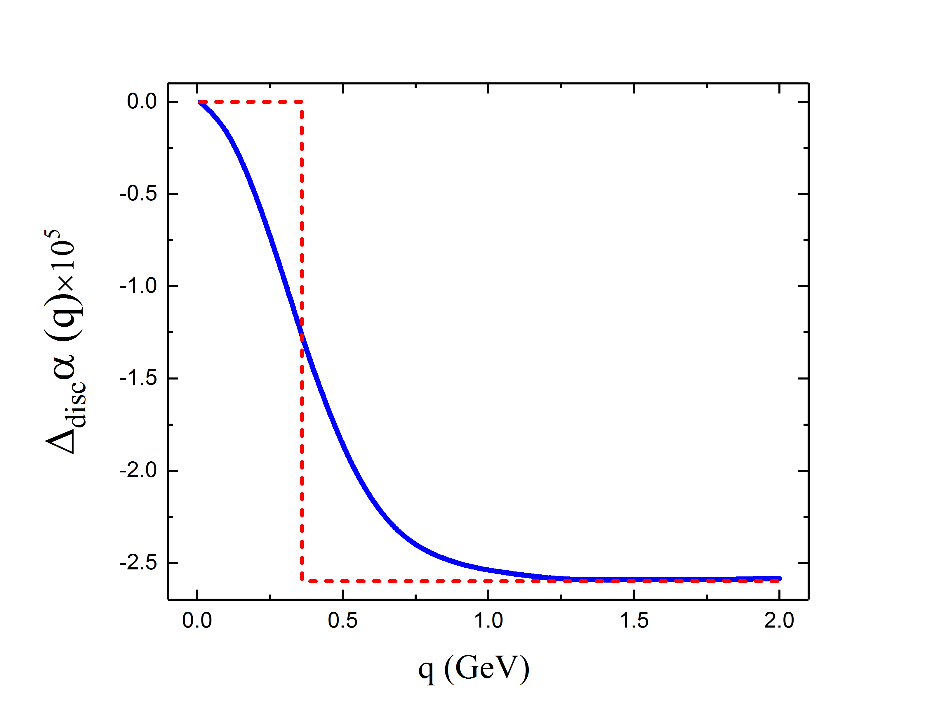
In Appendix B we compute $\Delta_{\rm disc}\alpha$ in the on-shell scheme by exploiting the lattice gauge theory calculation [23] of the corresponding contribution to $a_{\mu}$ with the result,

Note that because the sum of the charges of the three light quarks vanishes, and we enter the perturbative domain where the singlet piece is known to be tiny, we expect an asymptotically stable value at higher energies for $\Delta_{\rm disc}\alpha(q)$. This is supported by Figure 2, showing that $\Delta_{\rm disc}\alpha(q)$ is nearly $q$-independent for $q\gtrsim 1.2$ GeV. We also remark that the dominance of low scales notwithstanding, the sign in Eq. (29) coincides with that of the singlet piece in the perturbative regime. Also shown in Figure 2 is the step function approximation of $\Delta_{\rm disc}\alpha(q)$, with the step defined as the value of $q$ where it reaches half of its asymptotic value in Eq. (29). We interpret this as the value where the strange quark decouples from singlet diagrams, so that $\bar{m}^{\rm disc}_{s}\sim 350$ MeV. Our central value of $\bar{m}_{s}$ to be derived in the next section, $\bar{m}_{s}=342$ MeV, is numerically very close to this providing evidence for $\bar{m}^{\rm disc}_{s}\approx\bar{m}_{s}$.

Eq. (28) and Eq. (29) refer to quantities in the $\overline{\mbox{\small MS}}$ and on-shell schemes, respectively, and in general these may differ. However, since we are working here in the three quark theory and the sum of the charges of three light quarks vanishes, the change of schemes is trivial. We can therefore use Eq. (29) in Eq. (28) and obtain,

where the uncertainty combines the errors from Eq. (28) and the one induced by the lattice calculation [23].

In this section we perform a flavor separation of the contributions of up-type from down-type quarks, or — given that up and down quarks are linked by the approximate strong isospin symmetry — a separation of $s$ from $u$ and $d$ quarks. Our strategy consists of first using exclusively the experimental electro-production data as tabulated in Ref. [16] to constrain the contribution $\Delta_{s}\alpha$ of the strange quark to $\Delta\alpha$. We then exploit the lattice gauge theory results in Refs. [18, 19] to confirm and refine the purely data driven analysis. Then we introduce the threshold mass $\bar{m}_{q}$ of a quark $q$ as the value of the ’t Hooft scale where the QCD contribution to the corresponding decoupling relation becomes trivial. $\bar{m}_{c}$ and $\bar{m}_{b}$ are treated in perturbation theory, while for $u$, $d$, and $s$ quarks we derive bounds using phenomenological and theoretical constraints.