Signatures of partition functions and their complexity reduction through the KP II equation
Abstract.
A statistical amoeba arises from a real-valued partition function when the positivity condition for pre-exponential terms is relaxed, and families of signatures are taken into account. This notion lets us explore special types of constraints when we focus on those signatures that preserve particular properties. Specifically, we look at sums of determinantal type, and main attention is paid to a distinguished class of soliton solutions of the Kadomtsev-Petviashvili (KP) II equation. A characterization of the signatures preserving the determinantal form, as well as the signatures compatible with the KP II equation, is provided: both of them are reduced to choices of signs for columns and rows of a coefficient matrix, and they satisfy the whole KP hierarchy. Interpretations in term of information-theoretic properties, geometric characteristics, and the relation with tropical limits are discussed.
Mario Angelelli
Department of Mathematics and Physics
“Ennio De Giorgi”, University of Salento and sezione INFN,
Lecce 73100, Italy
Keywords: Statistical amoeba, soliton, determinant, complexity.
MSC: 15A15, 35C08, 82B05
1. Introduction
The concept of partition function encodes in a single object the statistical data compatible with the physical constraints of a system, e.g., conservation laws. Hence, it explicitly connects its probabilistic and physical characteristics. This is a fundamental principle in the investigation of composite systems [34, 21] and is now applied in many different branches of sciences [32]. The basic form of the partition function involves a sum of exponential terms
| (1.1) |
where is Boltzmann’s constant, is the temperature, are the energy levels labelled by an indexing set and are the associated degenerations.
In practice, the implementation of this approach is limited by the intrinsic complexity of the model, since there are few cases where the partition function can be evaluated exactly, e.g., in a closed form [6]. Indeed, many phenomena in complex systems cannot be reduced to their individual components, thus (1.1) involves collections of objects and, consequently, the complexity of the calculation grows exponentially with the size of the system.
The occurrence of exact formulas for the partition function implies relations between the characterizing quantities of the system, e.g., correlation functions that are generated by the partition function through derivation. This gives rise to a family of differential equations whose compatibility follows from the existence of the partition function. On the other hand, one can start from a family of differential equations and look for their compatibility. This naturally leads to the investigation on connections between the partition function formalism and the concept of integrability, especially integrable hierarchies. In such a context, the role of the partition function is similar to the notion of -function, which provides one with a unifying framework for hierarchies of nonlinear partial differential equations and their remarkable behaviours, e.g., symmetries, infinite family of commuting flows, soliton solutions [28, 25].
Explicit links between the partition function formalism and integrable systems have already been identified and used to provide fundamental techniques in modern theoretical physics [6]. Remarkably, certain solutions of integrable PDEs can be interpreted as potentials, such as the Witten-Dijkgraaf-Verlinde-Verlinde (WDVV) equations in topological quantum field theories. A solution for the WDVV system defines a free energy for this theory, namely, a function which generates correlators by means of derivation [19].
Recent studies have been devoted to the combinatorics underlying these kinds of structures. One of most fruitful examples is the Kadomtsev-Petviashvili II (KP II) equation
| (1.2) |
where denotes the partial derivative of with respect to . The KP II equation is one of most important -integrable PDEs and is considered a universal model of two-dimensional integrable evolutionary equations. The combinatorial structures arise, for example, taking into account particular classes of solutions of the KP II equation, such as soliton solutions of determinantal (Wronskian) type [25]. These solutions are parametrized by points in the real Grassmannian space and their regularity and algebraic features have been extensively studied in the last years [8, 13, 16, 33, 1].
The aim of this work is to explore these requirements starting from a statistical perspective: we choose a class of combinatorial configurations related to sums of exponentials that generalise (1.1). Then, we investigate the information content encoded in constraints through the reduction of the class of allowed configurations. This purpose will be realised extending the method of statistical amoebas introduced in [5], i.e., considering a family of discrete “deformations” of the partition function and focusing on those that are compatible with some given constraints. A statistical amoeba is obtained relaxing the assumption of positive degenerations in (1.1). Negative degenerations of energy levels can be related to an imaginary part of energies and, hence, used to describe metastable states [35, 41]. This approach has proved useful in statistical physics, where the locus of zeros of complex-valued partition functions is employed in the analysis of phase transitions [36, 37, 35, 41, 9, 14]. In our context, the partition function is real-valued, but indefinite signs for degenerations open up the way to the study of stability (), instability ) and phase transitions ().
In general, the requirement of compatibility of the choices of signs for with a given constraint affects both the number and the form of allowed configurations. We will focus on determinantal relations, where the complexity of calculations of determinants is polynomial via Gaussian reduction (while other immanents, in general, have exponential complexity [45]), and integrability, which reduces the complexity through the occurrence of conserved quantities. We stress this point referring to the construction in [5], where all the combinations of signs for the exponential terms in the partition function are allowed, as a free statistical amoeba. On the other hand, restrictions on the allowed combinations of signs give rise to a constrained statistical amoeba.
A strong relation between determinantal relations and integrability has been established by Sato (see, e.g., [44] and further developments in [40]), where an expansion in terms of Schur functions is found to be a -function for the KP hierarchy if and only if its coefficients satisfy the Grassmann-Plücker relations [23, 29]. This has led to intensive research on equivalent reformulations of the KP hierarchy such as these involving the infinite Grassmannian [44, 40]. Whilst sharing some concepts with these issues, the present investigation is devoted to families of functions generated by a special class of solutions of the KP equation. It should be remarked that we concentrate only on the first equation (1.2) in the hierarchy for what concerns constraints reducing the complexity, and that we work in finite dimensionality. Moreover, the construction of statistical amoebas does not rely only on the global (determinantal) form of the initial function, but also on the individual terms in its expansion, because the generation of other functions goes through changes of signs for a given expression of the type (1.1). The consistency check with constraints and the construction of allowed configurations depend on relations between non-vanishing terms.
When we start from solitons in Wronskian form, the constraints come either from the determinantal relations or from the fulfilment of the KP II equation. In fact, we will see that both these assumptions reduce the allowed combinations of signs to the same family, i.e., the set of transformations that can be obtained by flipping the signs of some rows and/or columns of a coefficient matrix : this is showed in Theorem 11. The complexity reduction takes place because the information about the chosen signature for the terms in the exponential sum, which are labelled by subsets of , is stored in the elements of : in general, this presentation is non-unique due to a certain equivalence relation (Proposition 15). The connection with other equations in the hierarchy follows from the special form of the transformations in this family (Theorem 12).
The main scope of this work is the formal derivation of the above-mentioned properties. However, it is important to highlight potential applications of this approach: for instance, choosing a coefficient matrix and constructing the corresponding soliton solution, one can encode a sequence of “bits” in the signs of the pre-exponential terms, and recover a special family of sequences checking that the KP II equation is satisfied. We will quantify the information content following from the check of the KP II equation through the Kullback-Leibler divergence between two probability distributions on the strings of signatures. These results also have geometric implications, and we will briefly discuss the links with oblique projections and their statistical relevance. Likewise, we will point out the connection with the tropical limit in statistical physics as introduced in [3] and developed in [2]. These issues could be of interest for a better understanding of the relation between statistical physics, complex systems and learning methods [7, 31, 38]. We will outline some of these connections and postpone their detailed study to a separate article.
The paper is organized as follows: in Section 2 we fix the notation and summarize the basic notions that provide a starting point for our investigation. In Section 3 we introduce the link between soliton solutions of the KP hierarchy and statistical amoebas, generalizing the latter to higher dimensions. The occurrence of a particular structure to be preserved in the construction of statistical amoebas is the focus of the next sections: in Section 4 we prove that the compatibility of a choice of signs for the coefficients of exponential terms with the KP II equation implies that it is induced by rows and columns sign flips for a coefficient matrix. In Section 5 we consider the number of distinct configurations that can be obtained in this way. The relation with the strata of the corresponding free amoeba [5] is considered in Section 6. Two applications of the present framework are addressed in Section 7: the information content in the KP II constraint is studied via the Kullback-Leibler divergence (Subsection 7.1), while an intersection property is discussed in geometric terms (Subsection 7.2). Finally we draw conclusions and address some issues of potential interest for future investigations in Section 8.
2. Preliminaries
We briefly summarise the basic state of the art regarding Wronskian soliton solutions of the KP II equation and the statistical amoeba formalism which will be used in the rest of the paper. Before that, it is worth introducing some notations to enhance clearness.
2.1. Notation
In the following, we will denote by the power set of , by the collection of subsets of with elements and by the symmetric difference of . We will also use the notation ,
| (2.1) |
and, similarly, , , , etc. The expression implicitly assumes that , and , unless , in which case we have .
The symbol (respectively ) is the maximal minor of (respectively, ) whose columns (respectively, rows) are indexed by . We will occasionally use instead of for the sake of clearness. When a permutation of is involved, an additional sign comes from the parity of the number of inversions induced by on . Particular attention will be paid to the set of pivot columns , which is the least element of (with respect to the lexicographical order) associated with a non-vanishing minor .
The -Vandermonde matrix relative to real parameters is . The determinant of a general (not necessarily maximal) minor of is
| (2.2) |
So has maximal rank in cases of pairwise distinct soliton parameters , as we will assume. We will look at exponential sums whose terms also depend on variables , , where , , and .
The real Grassmannian is the space of -dimensional linear subspaces of a -dimensional vector space over . It can be presented as the quotient of the space of -dimensional frames in by the left action of . If denotes the set of real ()-matrices of maximal rank , one gets
| (2.3) |
where acts as left multiplication. Greek indices will often represent columns, while Latin indices will be used to label rows. Additional notation will be introduced in specific paragraphs.
2.2. KP II equation and Wronskian solutions
Determinantal solitons define a distinguished class of solutions that can be derived from Hirota’s direct method [28, 25] introducing derivatives acting on pairs of functions:
| (2.4) |
So one can rewrite the KP II equation (1.2) in the following homogeneous bilinear form
| (2.5) |
By the same token, one can rewrite the other equations of the KP hierarchy in bilinear form [28, 40]. The tau-function of the KP equation is related to via
| (2.6) |
It has been shown (see, e.g., [24]) that the Hirota derivative (2.4) can be characterized as a derivative operator with gauge invariance under the simultaneous action and , i.e.,
| (2.7) |
for any linear function of . This is manifest in the antisymmetric form of in (2.4) and is also reflected in the expression of a special class of solutions [25]
| (2.8) |
where , , are independent solutions for the following system of partial differential equations
| (2.9) |
One can take a certain number, say , of solutions of (2.9) in the form
| (2.10) |
with real parameters . A particular choice of solutions of (2.9) comes from linear combinations of these exponentials, with coefficients given by the entries of a matrix : , that is . One has
| (2.11) |
where . Finally, the resulting soliton solution is equivalently expressed using the Cauchy-Binet expansion [29] as
| (2.12) | |||||
| (2.13) |
It should be remarked that the left action of on , i.e., the multiplication of by a full-rank real matrix, induces the multiplication of by a constant and, hence, leaves solutions (2.6) invariant. Such an action is equivalent to row operations on , thus soliton solutions are parametrized by points of the real Grassmannian [29] rather than points on (see, e.g., [8, 16, 33]).
The solution (2.6) is regular at . If , then is multivalued, but its imaginary part does not depend on and disappears after derivation in (2.6). Thus, possible singularities of soliton solutions are related to the points where vanishes. If the order for soliton parameters is fixed, then the locus of zeros of is not empty if there exist maximal minors with opposite sign, i.e., if parametrises a point outside the totally non-negative part of the Grassmannian [33].
2.3. Statistical amoebas
The analysis of roots of the partition function is a fundamental technique in the study of stability, metastability and phase transitions in composite systems [36, 37, 41, 14]. Finite sums of exponentials of the type (1.1) are positive for real values of energies and temperature and positive degeneracies . So the zeros of the partition function define a singular locus in the complex domain and, in many cases, they approach the real line when the number of terms involved in (1.1) becomes large (thermodynamic limit).
If one restricts to the real domain, the partition function can vanish if not all the degeneracies have the same sign. This corresponds to real partition function of indefinite signatures and relates to the concept of negative probabilities [46, 18, 20, 11]. This proposal has been developed in [5] for partition functions of the type
| (2.14) |
where the functions represent “micro-free energies” that depend on certain parameters (e.g., temperature, external magnetic fields, etc.). When one fixes , the -stratum of the statistical amoeba consists of the zero loci of the functions produced by any possible combination of signs among the terms in (2.14), i.e., with . In great generality, that is under the only assumption of polynomial functions , , a pattern can be found in the study of the singular locus: the -stratum is confined in a region of the space of parameters , and the instability domains obey the following inclusion property
| (2.15) |
The restriction also avoids the redundancy given by the simultaneous reversal of all the signs. This is equivalently expressed via the involution , which preserves the singular locus and exchanges the role of equilibrium () and non-equilibrium () regions, since . Thus, the strata associated with are said to generate the statistical antiamoeba.
When all the combinations of negative coefficients are taken into account, the set coincides with the locus of points where the maximal number of negative partition functions (2.14) is obtained. This maximum is the same for all the systems with polynomial and equals . Furthermore, the polynomial assumption is also suitable for the study of the tropical limit [3, 5], both in the linear and in the nonlinear cases (the latter is referred as a multi-scaling tropical limit [4]).
3. From soliton solutions to statistical amoebas
The explicit form of many soliton solutions of partial differential equations can be derived from a sum of exponentials [28]. In order to highlight the relation between statistical amoebas and -functions, it is worth noting that the partition function (1.1) can be expressed as
| (3.1) |
where , and . In particular, is a totally positive vector (all its entries are positive) and can be interpreted as a Vandermonde matrix. This formula for the partition function coincides with a Wronskian -function (2.12).
More generally, we can express such a type of -functions as a sum of exponentials through the Cauchy-Binet expansion of the determinant of a product: if one introduces
| (3.2) | |||||
| (3.3) |
then (2.13) is of the form (2.14),
| (3.4) | |||||
In this way, we move from degenerations multiplicities to more general products of minors . The dimension , which coincides with the rank of and when does not identically vanish, indicates the number of line solitons at , while is related to line solitons at . In the statistical perspective, is the partition function for a statistical model whose configurations correspond to subsets and have energies . If and is a matrix with integer entries and maximal rank, then (3.2) is an integer, and can be seen as degenerations for independent events and is the joint degeneration. The th column of generalizes in (1.1), so it can be regarded as a degeneration vector relative to the th energy level , .
Regularity hypotheses for the case can be extended to -functions at too. For example, the entries of in (1.1) and (3.1) are assumed to be positive since they are a measure for degenerations associated with energy levels. At , this property generalizes to a real matrix where all the maximal minors are non-negative. If one fixes the ordering for soliton parameters, then this request guarantees (indeed, it is equivalent to, see e.g. [12]) the positivity of the Cauchy-Binet expansion (2.13), hence the regularity of the solution of the original KP II equation.
In the next section, this kind of request will be relaxed: the matrix is only assumed to obey the full-rank condition. However, some peculiarities of the total non-negative case will be discussed in Section 6.
Definition 1.
A choice of signs, or signature, is a map
| (3.5) |
where
| (3.6) |
acts on (3.4) via , which returns a new function
| (3.7) |
The set is a matroid on : this means that the exchange relation holds, i.e.,
| (3.8) |
In particular, we refer to a generic case as one where .
4. Complexity reduction through the KP II constraint
The determinantal partition function (3.1) at reduces to the statistical amoebas studied in [5]. Cases at have more complications, due to the occurrence of functional relations among the terms in the -function (3.4). Indeed, the minors of a ()-matrix have to satisfy the well-known Grassmann-Plücker relations (see, e.g., [23], §3.1). In particular, the three-terms Plücker relations
| (4.1) |
hold for all and with and .
Example 2.
For a generic matrix , , not all the signatures (3.5) for in (3.4) correspond to another choice of matrix in (3.2). In fact, consider such that there exist two non-vanishing minors and , e.g., taking parametrizing a point in the totally positive part of the Grassmannian . Suppose that the choice
| (4.2) |
which lies in the free statistical -amoeba relative to (3.4), corresponds to a certain matrix . The relation (4.1) gives
| (4.3) | |||||
that means , a contradiction. It follows that, for points in the totally positive Grassmannian, no signature of the type (4.2) preserves the form (2.8).
In general, it is not a trivial task to check if a given map of the type (3.5) follows from maximal minors of a certain matrix. This issue is related to combinatorial structures behind Grassmann-Plücker relations, namely chirotopes (see, e.g., [43, 10] for more details). In particular, chirotopes coming from , in the sense that for all , are said to be realizable. Both the check of the realizability of chirotopes and their enumeration have non-trivial complexity [26]. However, in the present framework, the data on the initial function, in particular the “lengths” of the exponential and pre-exponential terms, are given: starting from (3.2), these absolute values are known to be compatible with at least one determinantal (Wronskian) form, and can be used to explore other signatures.
We exclude situations where (3.4) identically vanishes, so has maximal rank and there is no null row . If there exists a null column, then the -function does not depend on the corresponding soliton. This leads to the reduction of a - to a -soliton solution. So we can assume that there is no null column without loss of generality.
We now consider the conditions on choices of signs that map a -function of the KP II equation (2.5) to another -function, which will be called solitonic signatures. Let (3.5) be any choice of signs for coefficients in (2.13), which is equivalent to a choice of a partition of in two disjoint subsets , , where
| (4.4) |
So one can write the resulting exponential sum as
| (4.5) |
where
| (4.6) |
Moreover, we will say
| (4.7) |
which defines a relation on .
We do not assume a priori that a partition (4.4) returns a determinant (2.8): this means that the determinantal properties (i.e., Grassmann-Plücker relations) hold for the family , but not necessarily for .
The bilinearity of the Hirota derivative and the KP operator (2.5) gives
| (4.8) | |||||
since . Therefore, one has
| (4.9) |
We can say that is “orthogonal” to with respect to the bilinear operator. The bilinearity also implies that (4.9) is equivalent to
From
| (4.11) | |||||
where
| (4.12) | |||||
The equation () is equivalent to
| (4.13) |
Two exponentials in (4.13) associated with the pairs and identically coincide if and only if
| (4.14) |
The only occurrences of (4.14) that are satisfied for a generic choice of the parameters involve the cases when and . So, if one assumes that there is no algebraic dependence that relates these sums when or , then each exponential term in (4.14) is determined by the union and the intersection , since
| (4.15) |
In particular, one has the following
Lemma 3.
- Proof:
Suppose that there exist subsets , such that , , and , so the number of terms in (4.13) associated with and is not . In particular, . Then, there exist and such that . There are two additional pairs of subsets different from with the same union and intersection. Thus, in order to have a vanishing coefficient for the associated term in (4.13), at least one of these two pairs has to belong to . Let us suppose that only one of these two possibilities is in , call it with . In such a case, the term in (4.12) is
(4.17) that is not vanishing since the soliton parameters are pairwise distinct by assumption. Using the parity of the permutation , we introduce
(4.18) which gives
(4.19) The signs and can be found in the same way, taking into account that
(4.20) Furthermore, one can consider
(4.21) where . In this way, it is easy to check that
(4.22) where is the product of and the parity of the permutation . Thus, one gets
(4.23) The first term in braces in (4.23) is the same for all the pairs with and . For the second term in braces, the antisymmetry (4.20) implies that
(4.24) The three-terms Plücker relations (4.1), which are valid for minors , can be stated for any four pairwise distinct elements , , as
(4.25) In particular, if one looks at the sum of (4.23) and (4.24) and applies (4.25) with , the result is
(4.26) since we have assumed that all the minors are not vanishing. Hence, the coefficient in (4.13) associated with and is not vanishing and the associated -function is not a solution of the KP equation (2.5).
Proposition 4.
Let , and such that . Then at least one of the two products , , is not vanishing. Further, if , then .
- Proof:
First suppose that one of the product vanishes, e.g., without loss of generality. Then the three-terms Plücker relations (4.1) imply that . Further, implies that there is exactly one non-vanishing term in (4.13) associated with a pair in with intersection and union , hence (4.27) do not vanish. Thus . If instead both and are not vanishing, then (4.16) holds because of Lemma 3 (see in particular (4.26) and (4.27)). ∎
Lemma 5.
Let with . Then there exists a finite sequence of elements of such that , .
- Proof:
Let and , so the exchange property (3.8) implies that there exists such that . Note that . One can iterate the process, starting from and finding in order to define
(4.28) such that too. At each step, the element is different from for all because , while . So the map is injective and, hence, a bijection, since implies . All the subsets are elements of and for all . ∎
Now we consider the following relations
| (4.29) |
If there is such that where , then one can express as . This does not depend on the choice of , as can be easily shown:
Remark 6.
Let and . Then holds for a certain if and only if holds for all such that .
- Proof:
In fact, the relations (4.29) are compatible for different choices of too.
Proposition 7.
There are no subsets , , and such that and .
- Proof:
Introduce , , , . Note that , and .
We shall prove the statement by induction on the distance between and , that is . First consider the case and set . In particular, the elements are all distinct and the set satisfies , , and . By hypothesis, , so Proposition 4 gives . Multiplying both sides of this equation by and applying we find
(4.30) Now assume that the statement holds whenever and take , with . From Lemma 5 there exist a labelling and two bijections , , such that
(4.31) Let us focus on the four sets , , , : by hypothesis, and by construction. Further, one has and . Since the distance between and increases by at each step, one gets . So the inductive hypothesis applies and
(4.32) Likewise, , and , so one can repeat the same argument as in (4.30) and get
(4.33) Multiplying (4.32) and (4.33) side by side, and applying , one finds
(4.34) that means if and only if . ∎
Hence, for each , the relation (4.29) depends only on and , and not on such that . If such a exists, we can introduce
| (4.35) |
without ambiguity. Moreover, is symmetric in its arguments, since and one can substitute in (4.35).
We will see that the signs (4.35) characterize , so we focus on these pairs.
Definition 8.
For each take the matrix defined as if and otherwise (). We refer to a path on as a sequence of non-vanishing entries obtained moving alternately along rows and columns of , i.e., of the form
| (4.36) |
with , and for all . Two indices are said to be connected by a path if is a component of the first element of but not of the second, and is a component of the last element of but not of the second-to-last.
For instance, if and , then a path from to starts with and ends with , for some ; if instead both and are elements of , a path starts with and ends with , . These paths induce a relation on .
Definition 9.
For all , we say if or there is a path in that connects and .
This is an equivalence relation: it is reflexive by definition; if , then the reverse path gives , so is symmetric; it is also transitive, as follows from the path obtained from the concatenation of and and the simplification of consecutive reverse subpaths. Moreover, the following result holds:
Proposition 10.
The product of signs of edges along any closed path of , , is .
- Proof:
Let and denote by in the rest of the proof for the sake of clearness. The same number of moves along rows and along columns is required to close a path, so it has an even length . Thus, the product of signs along the closed path is
(4.37) where indices are taken modulo , e.g., . From this one can also see that the statement is invariant under the replacement of by , as long as all the involved subsets and are in : indeed, both sides of (4.37) can be multiplied by , so the factors are expressed as (respectively ) by Proposition 7.
We prove the statement by induction on . The base cases are , which is trivial by symmetry of with respect to the interchange of its arguments, and . In the latter situation, there exist and such that . By Proposition 4 the associated product of signs is . Now assume that the thesis holds for and take any path of length . First suppose that there exist , , such that . Then one can write
The lengths of these two closed path are and respectively, which lie in ; so the inductive hypothesis applies to both these paths and this gives the result.
On the other hand, if such do not exist, then for all and : by Proposition 4, the condition , along with at and at , implies that for all . Likewise, from , () and (), one gets whenever . Further, and lead to for all .
So we fix : by previous observations, one has for all , and . One can apply Proposition 4 to and , which are in , and write
(4.39) Thus consider the path of length on , which also satisfies for all (all the subsets are in and Proposition 7 holds) and by (4.39). Since the involved subsets are in , the inductive hypothesis applies to the path in and that gives
(4.40) ∎
A special role is assumed by the pivot set , since the hypothesis of no-null columns implies that each is associated with an element (possibly ) such that . So we can finally state the main result:
Theorem 11.
A choice of signs returns a solution of the KP II equation (2.5) if and only if is induced by a choice of signs for rows and columns of (up to the action of ).
- Proof:
One implication is trivial, since a choice of signs for rows and columns of induces a (singular) soliton solution by construction. So consider any choice of signs that returns a solution of the KP II equation and choose an arbitrary element in , e.g., . For each and , given that , the Plücker relations imply that there exists at least one non-vanishing term of the type . Thus one can always find such that both and are elements of . So let : as in Lemma 5, we start with and, from and , , we find
(4.41) such that . Also in this case, from for all and , it follows that all are pairwise distinct. So we get
(4.42) Now consider the equivalence . Each class contains at least one element , since we have assumed that there are no null columns: fix a sign for each of them. For any , take a path on connecting and , and set
(4.43) This definition is well-posed since it does not depend on the choice of the path by Proposition 10. If , then belongs to the same class of , because the path with only one element connects them. The concatenation of , the reverse of and makes a closed path, whose product of signs is equal to by Proposition 10. So
(4.44) Finally, since , we can express as
(4.45) where
(4.46) Hence is induced by a choice of sign for columns and for an arbitrary row of . ∎
The previous results can be summarised in the following theorem, which relates the requirements coming from the determinantal form (3.1), the KP II equation and the whole KP hierarchy.
Theorem 12.
- Proof:
A choice of signs (3.5) returns a solution of the KP II equation (2.5) if and only if it is induced by a choice of signs for rows and columns of by Theorem 11. In this case, the associated function is a solution of the whole KP hierarchy.
If we focus on the determinantal structure of the -function, all the choices of signs for rows and columns clearly preserve the form (2.12). On the other hand, if a signature preserve this structure, then the KP II equation is satisfied (together with all the other members of the hierarchy). So, from Theorem 11, this solution can be expressed in terms of the initial function via a choice of signs for rows and columns of . ∎
A more detailed analysis on the signatures preserving the determinantal constraints, which also includes the preservation of a specific subset of soliton parameters, is given in Appendix A.
A special situation is when is defined over the whole set , i.e., . In such a case, one can easily verify that Remark 6 implies that is an equivalence. If some vanishing minors occur, then the transitivity of the relation (4.29) is not guaranteed. So one could look for a transitive extension of all the relations at varying . An extension of , that is a map that satisfies for all , can be obtained using (4.43) to label minors in with a sign compatible with Proposition 4. So the following holds:
Corollary 13.
For a solitonic choice of sign , there exists an extension of to the whole set such that is a solitonic choice of signs too.
It could be interesting to extend this approach to more general expressions for the -function and to other hierarchies, in order to check the complexity reduction coming from the initial data and the specific requirements.
5. Number of distinct configurations
Having identified a family of signatures that preserve specific requirements, it is worth exploring some of its combinatorial aspects in order to clarify the effects of the initial data, e.g., the coefficient matrix , on the set of allowed configurations.
The overall sign given by row signature is obtained with the choice for an arbitrary row of (see (4.46)). Sign flips for columns can be expressed as an action of on by right multiplication, i.e., and where
| (5.5) |
Accordingly, (3.4) becomes
| (5.6) |
If , then the minors of are the entries of a row vector. Then, for every non-zero matrix such that for all , one can recover from (5.5) choosing . If , such a choice is unique. The use of (5.5) in the case gives a suitable generalization.
Lemma 14.
Let and be the equivalence classes associated with the relation in Definition 9. For all , the equalities
| (5.7) |
imply that there exists such that
| (5.8) |
- Proof:
First note that the condition (5.7) holds for if and only if it holds for : indeed, for all , and have the same set of non-vanishing maximal minors and, in particular, the action of does not affect the relation relative to the pivot set . In the substitution , the additional signs coming from , , appear on both sides of (5.7), then
(5.9) since . So (5.7) holds for the pair if and only if it holds for .
Take any class , , and two elements of . Then, there exists a path in , which consists of a chain of pairs , , associated with subsets . If the condition (5.7) holds for such subsets, one gets
for all . The concatenation of all these equivalences for all the pairs in the path gives the implication
(5.10) for all and , which is equivalent to (5.8). ∎
Thus the redundancy in the representation of signatures by subsets of is due to the elements of
| (5.11) |
Note that are pairwise distinct for different choices of since is a partition. This still holds for the elements in
| (5.12) |
satisfying (5.8), since the symmetric difference is invertible and, hence, the mapping is bijective.
Proposition 15.
- Proof:
For each subset consider a map constructed as in (4.41) that associates to a unique so that . This also implies . Thus, the non-vanishing minors of correspond to subsets which intersect all the classes and, in particular,
(5.13) does not depend on . Then, the involutions defined by
(5.14) act as follows
(5.15) Using the partition , one can uniquely express in terms of its components and get, for each , the following equalities
(5.16) Hence, if (as in (5.8)), then from (5.15) and (5.16) one gets
(5.17) Now choose any ancillary soliton parameter , introduce the matrix
(5.18) and denote the new column by the index . There exists a bijection between the non-vanishing minors of and those of , that is . Any choice of signs for the columns of , , can be extended to a choice for as . Furthermore, the choice in (4.46) is restated as a new signature for columns only, i.e., . Hence this equivalent model describes the original one using only column operations, up to a common multiplicative factor for the terms . The pivot set for is , and this extends the relation to the equivalence whose classes are and , since for all .
So there are choices of signs for the columns of and distinct equivalence classes for . The cardinality of one of them, i.e., , is odd: hence, from (5.15), the substitution induces the mapping
(5.19) for any subset . In conclusion, Lemma 14 states that, for each , the possible sets satisfying (5.7) lie in (5.12); each element of this family satisfies (5.17) independently on ; finally, from (5.19) it follows that each signature corresponds to the opposite one , so they occur in equal numbers. This means that exactly half of the terms in (5.12) have the same signature of , while the other half have opposite signature. Hence there are subsets associated with a single signature, and the number of allowed signatures is . ∎
Remark 16.
The previous discussion also implies that the sets (5.12) are equipollent and pairwise disjoint, since each of them contains all the possible combinations of subsets of that induce a given signature or the opposite .
The freedom in the choice of signs generalizes free statistical amoebas (including an additional row sign flip), which fall within the case . Indeed, let denote the number of distinct signatures induced by the sign flip of exactly columns of , , without limitations on . Each combination of signs for row and columns can be labelled by an element in , hence . At , produces the same signature of its complement for an appropriate choice of , so . These bounds, along with the action of (5.17) and the result in Proposition 15, give
Thus all the bounds are in fact equalities, i.e., at and .
6. Levels of constrained amoebas
The previous discussion leads to an extension of the concept of statistical amoeba to higher dimensional cases. Following the construction for free statistical amoebas in [5], one can focus on the family of functions (or the associated locus of zeros) obtained from through all the combinations of sign flips for columns at fixed.
We can associate with each the vector defined as if and otherwise. The intersection of is given by the componentwise product , hence the parity of is equal to the dot product
| (6.1) |
Motivated by this, we adopt the following notation
| (6.2) | |||||
| (6.3) |
and with and .
Unlike the free statistical amoeba at , only some strata are visible under choices of signs allowed by determinantal/integrability requirements. For instance, a single change of sign preserves neither the determinantal structure (see Example 2) nor the solution of the KP II equation in generic situations. Hence the -stratum for the free statistical amoeba is not part of the constrained amoeba.
Let us focus on the case . For all the choices of , and , the number of signs generated by is equal to the cardinality of . This holds for all possible choices of by permutation symmetry. The singular locus corresponding to is a subset of all the singular loci in the free -statistical amoeba.
Proposition 17.
- Proof:
Let . The number of subsets satisfying is
(6.6) where at or . We observe that is equivalent to
(6.7) where the principle of inclusion-exclusion has been used in the second line. So, at even (respectively, odd ), the enumeration of sets with is equivalent to the enumeration of subsets with (respectively, ). Furthermore, exactly one holds between or .
So we can look at the situations where and derive the required quantity in other cases by the previous observation. First note that
(6.8) counts the number of elements of . For the first summation, one has
(6.9) where is the Gaussian hypergeometric function, and all the equivalences are well-posed due to the condition . Adding the two contributions, we get . From this we also find that, at , the number of -subsets with is , while those with are . By (6.7) and subsequent observations, these two quantities respectively enumerate the number of -subsets with at even and at odd . These results can be expressed as in (6.4), which concludes the proof. ∎
It is worth remarking that there is a duality between the dimension and the level : the number of pairs such that can be enumerated in two ways, i.e., fixing one of the two components , and considering all the subsets with . This double counting implies the following identity
| (6.10) |
From this, one also finds
| (6.11) |
In this sense, the distinction between (free) amoebas and antiamoebas, as defined in Section 2.3, is compatible with such a duality. Furthermore, when for all , the quantity dual to is related to the behaviour of the constrained amoeba at large values of , namely, to its tropical limit [5]: outside the locus where is attained more than once, the sign of at coincides with the induced sign for this dominant term, that is . So represents the number of subsets where .
7. Applications
7.1. Application to information transfer via message coding
The previous results suggest using an initial function (2.13) to encode information. Specifically, we can think at each signature as a message encoded in a -bits string, where . Here we assume that the order of the bits in the string corresponds to a given (e.g., lexicographical) order for the elements of . Analogously, we can represent (2.13) as a string with entries in , where the entries label the minors of and the symbol is associated with vanishing minors.
If one knows that the original function solves the KP II equation and receive a new function , then the fulfilment of the KP II equation implies that a particular choice of signs has been sent. We stress that all the signs have to be checked to confirm that is induced by row/column operations: indeed, in the generic case , a single switch of sign converts a constrained signature to a non-constrained one, as shown in Example 2. However, in the present approach, one can check if is induced by a choice (5.5) indirectly, i.e., without having to find such a configuration and, hence, avoiding the effort to get this additional knowledge.
In order to quantify the amount of information that can be acquired through this single check, we consider the well-known Kullback-Leibler divergence [15]. After the reception of the message, but before any additional check on the signs, one can recover the data related to dependence relations among the columns of , namely , and, for any fixed , the relation and the dimensions . At this point, the prior information is based on strings of bits indexed by . With no additional constraint, we can assume a prior distribution where all the -bits strings have the same statistical weight . In the generic case there are such strings, but only of them satisfy the KP II equation by Theorem 11 and Proposition 15. This restricted family of strings associated with solitonic signatures is the support for the posterior distribution . So the Kullback-Leibler divergence is given by
| (7.1) | |||||
When , the number of distinct general strings is while the number of those satisfying the KP II equation is by Proposition 15. So one gets
| (7.2) |
which is a real non-negative quantity, hence we also find
| (7.3) |
In the previous cases, the assumptions of equiprobability for strings in and for choices of signs induced by (5.5) are consistent as a result of Proposition 15, since the equivalence classes associated to the different signatures are equipollent (also see Remark 16). One can get the quantities (7.1)-(7.2) through the choices , and , which reduces to the same multiple-counting of both general and solitonic signatures. This type of equivalence does not necessarily hold when further restrictions affect the prior. In particular, we consider a situation where the number for allowed is fixed and known, as in the discussion on statistical amoebas in [5].
In order to explore some features of this setting, we first estimate the information content associated with the check of the KP II equation in the generic situation . Let us look at the effects of the knowledge of a fixed value for at to avoid the occurrence of solitonic signatures related by the involutions (5.14) and, hence, to single out the contribution of the evidence on . This enables us to consider a preliminary check before looking at the KP II equation: if neither the received string nor its opposite satisfy , then is not obtained through (5.5) with and, hence, does not satisfy the KP II equation. Furthermore, at , also the row sign is fixed by this preliminary check, and this restricts the support of the uniform distributions for the prior and the posterior to and , respectively. The uncertainty on still remains at . So the Kullback-Leibler divergence is equal to
| (7.4) |
The last term, which involves the cases , does not appear if one also knows that only column operations can be performed.
We present a graphical representation of the Kullback-Leibler divergence at : the behaviour of (7.4) at different values of is shown in Figure 7.1, and can be compared with (7.1) in Figure 7.2. The analytic continuations of both these formulas have been used.
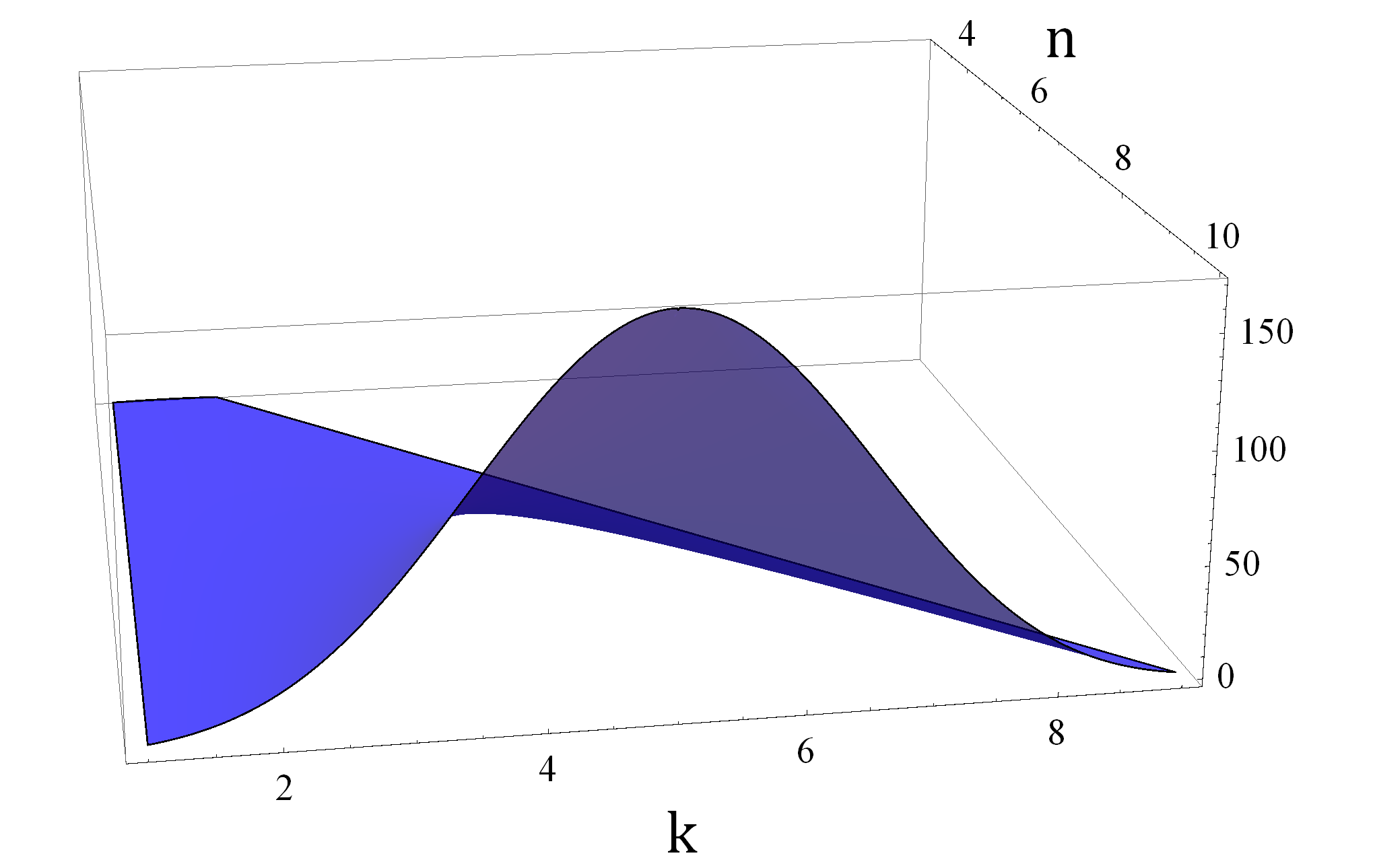
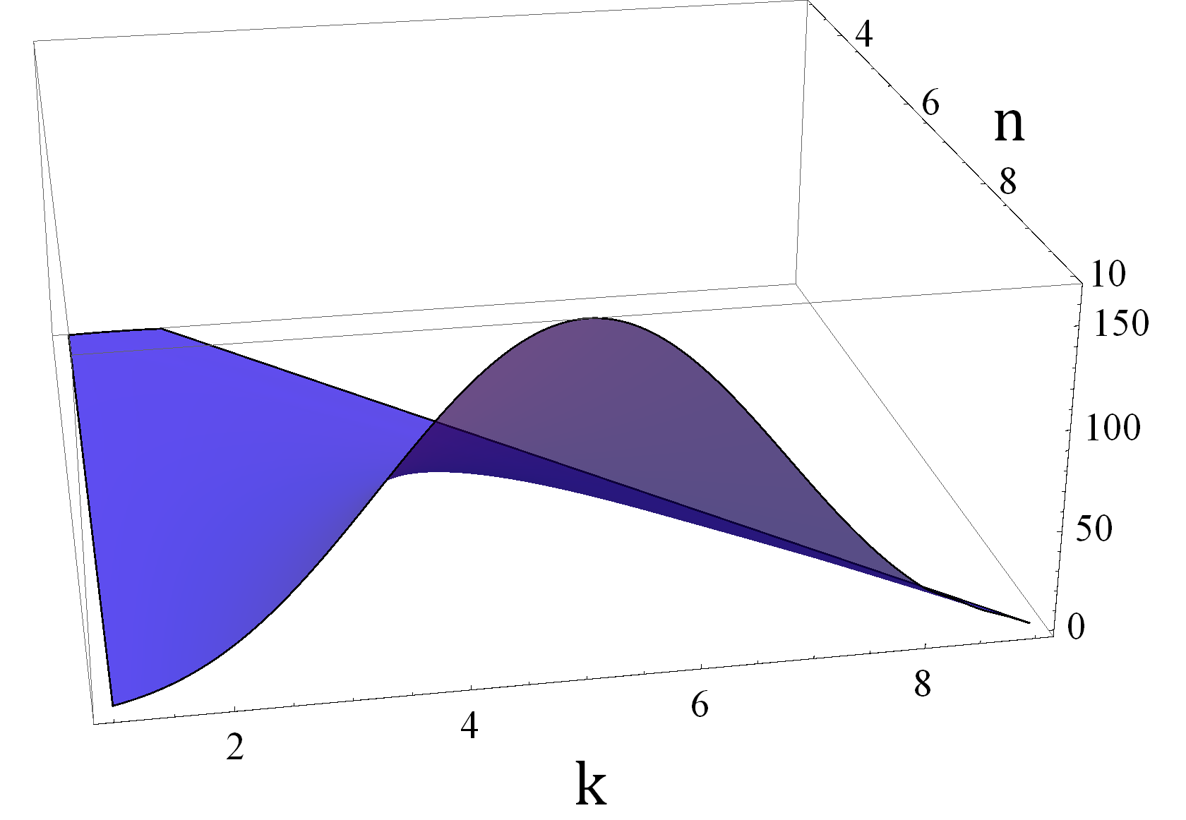
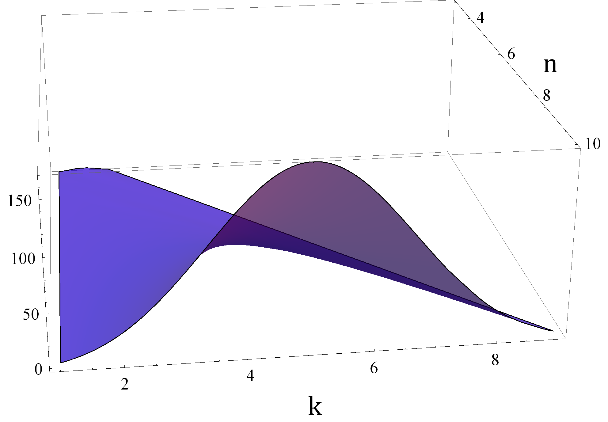
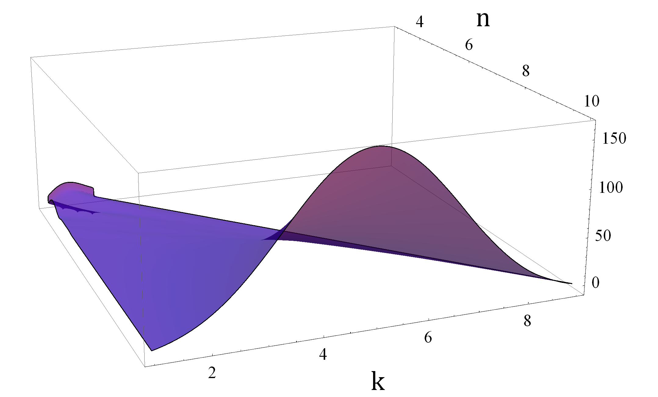
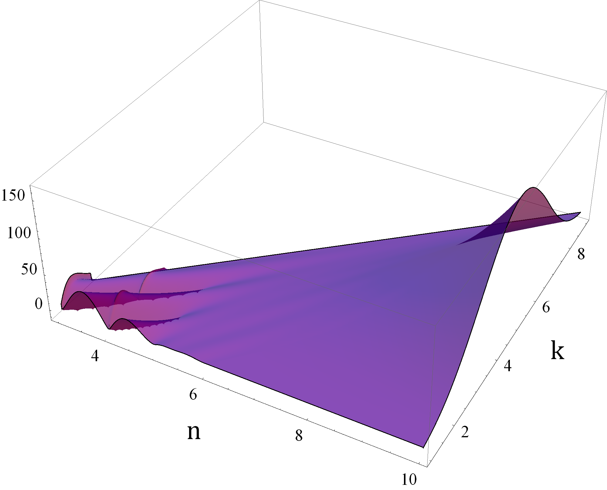
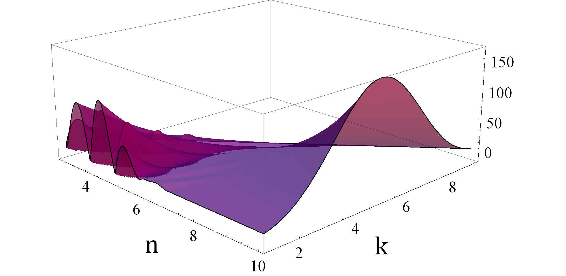
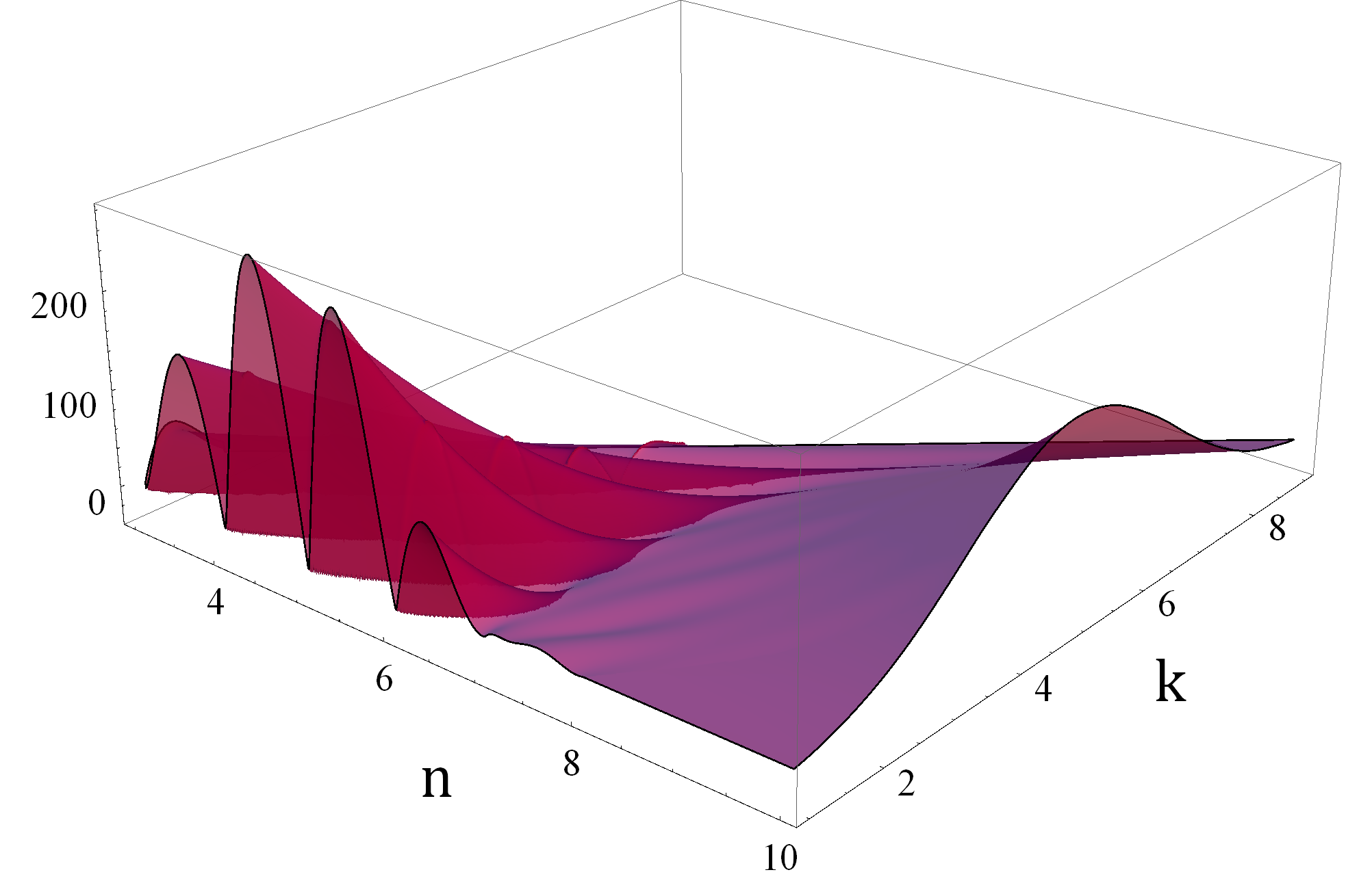
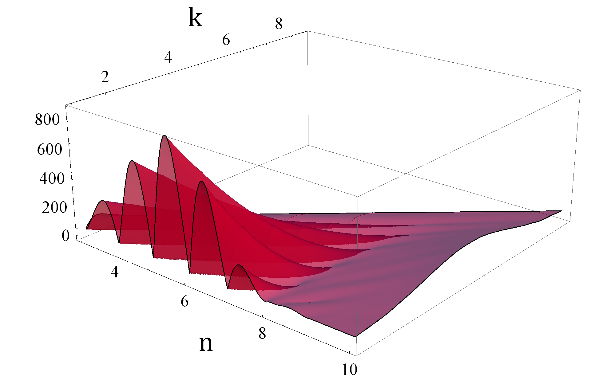
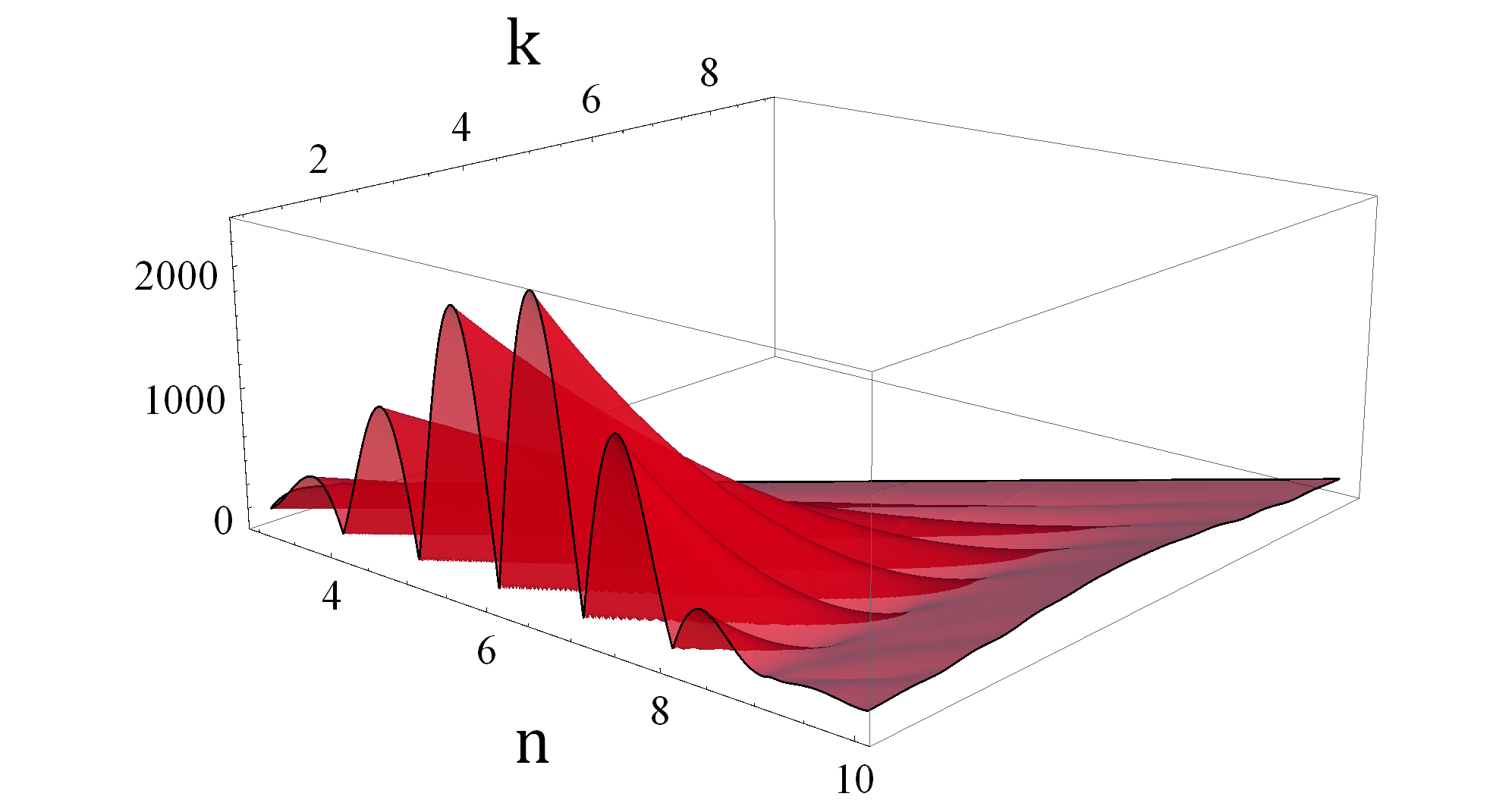
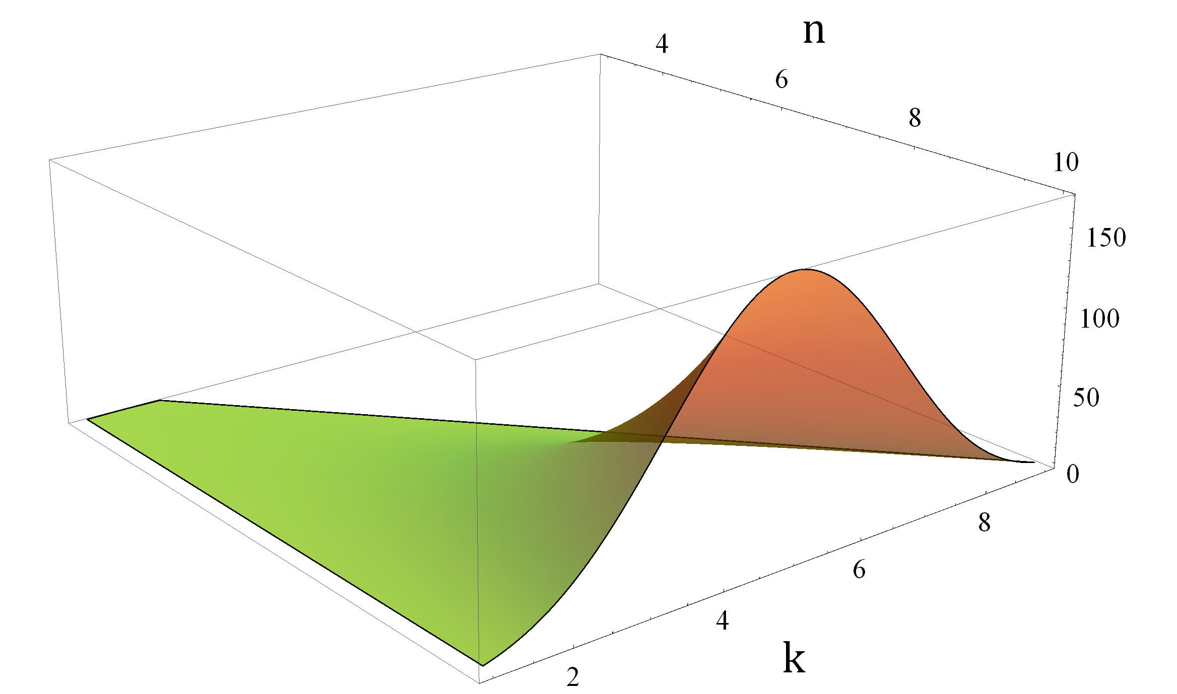
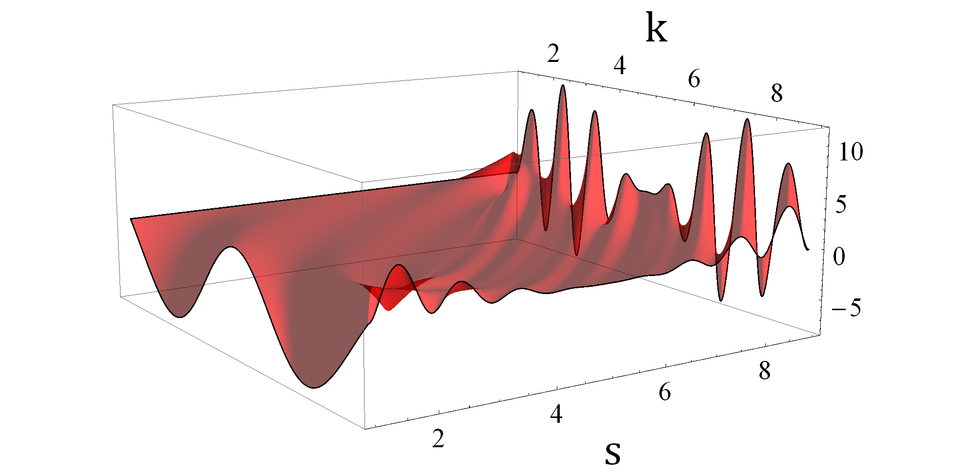
The gain or loss of information can be quantified by the difference (see Figure 7.2). It depends on the values , as shown in the following example.
Example 18.
Let us consider the generic case . At we find that , , and , so .
On the other hand, moving to the case , the quantities , , and , so .
In contrast to the generic case, situations where may exhibit different combinatorial features, and the equivalence between solitonic signatures (3.5) and the induced representations (5.5) is weakened. In particular, the constraint on the number of negative signs in does not correspond to a fixed number of signs for in (5.5), and vice versa. Furthermore, if one assumes a uniform prior distributions on in the construction of solitonic signatures by the sender, then it is natural to assume that the solitonic signatures are not equiprobable. In fact, moving from signatures in to elements of , the assumption that choices for occur with the same probability endows the associated -bits solitonic strings with multiplicity weights. Each weight expresses the redundancy of the representation (5.5) counting the number of subsets that induce the same signature. At fixed , these weights do not coincide for all the signatures in general. For instance, if there is no subset such that
| (7.5) |
then each involution (5.14) makes the index of the signature change. On the other hand, if (7.5) is satisfied, then both and have negative signs and induce the same signature. We clarify these issues through the following examples.
Example 19.
Consider the matrix
| (7.6) |
The non-vanishing minors for can be indexed by elements in , so , while it is easily seen that . Not all the choices in correspond to distinct signatures, due to coincidences from (5.14) and . In fact, there are distinct solitonic signatures associated with as many classes in a partition of , where each class includes all the subsets that returns the same signature. Assuming a uniform distribution on , we get the following induced distribution for solitonic signatures
| (7.7) |
The Kullback-Leibler divergence from the uniform prior over to (7.7) is . Note that the relative entropy, starting from but without the information on , is by (7.2). On the other hand, using (7.1) and (7.4), we find that and in the generic case. Thus, while the unconstrained case is favourable in the generic case, the unconstrained one may be preferred when .
Example 20.
Consider the matrix
| (7.8) |
It is easily seen that is a rectangular block matrix whose three blocks are full-rank Vandermonde matrices, call them . Thus one can enumerate the non-vanishing minors of as in the previous example and find .
First we note that the constraints on in (5.5) and on the negative signs in do not match: at , the choice returns a signature with negative signs, while gives negative signs. The operation (4.46) preserves the parity , since is even, so the choices and still have different parity when the choice for is included. Vice versa, a fixed number of negative signs for solitonic signatures does not correspond to the same constraint for : both and generate signatures with negative signs, despite having different cardinalities.
Let us focus on the case . Before undertaking any check on the signature, we choose a uniform prior on the possible ones. In contrast to Example 19, distinct choices of produce distinct signatures: indeed, two subsets inducing opposite signatures has to be related by the action of some involutions (5.14) respecting (7.5). But any operation of this type returns the same signature, since the ranks of the matrices are all even. However, also in this case the uniform distribution on induces a non-uniform distribution on the solitonic signatures: for instance, the signature associated with does not coincides with other ones, while and lie in the same equivalence class, and this results in different weights. Computing the relative entropy as in the previous example, one gets , while the unconstrained case gives .
The features of non-generic cases and the dependence on the parameters can be used to adapt the amount of information content in the two cases of unconstrained and fixed cardinality for in (5.5). A specific analysis in this regard will be carried on in a separate work.
7.2. Intersection property and its geometric interpretation
The introduction of the families
| (7.9) |
plays a significant role in the identification of the stratified structure of statistical amoebas at . This comes from a simple combinatorial property (see Proposition 5 in [5]), which can be extended to the case as follows.
Proposition 21.
If for all , then there are no pairwise disjoint sets in .
- Proof:
Let us suppose that such sets exist, i.e., such that for all . By definition, is equivalent to the inequalities
(7.10) Let us divide these subsets in two classes and . Adding the inequalities (7.10) for term by term, one gets
(7.11) Similarly, for one has
(7.12) If appears in the left hand side of (7.11) (respectively (7.12)), then it has non-empty intersection with more than elements in (respectively, . In the same way, if with and distinct , then . So and the coefficient of in the right hand side of (7.11) is . Since by hypothesis, this means that the right hand side of (7.11) is an upper bound for the left hand side of (7.12), which implies
(7.13) Arguing in the same way for (7.12), one gets
(7.14) which is incompatible with (7.13), i.e., a contradiction. ∎
The previous bound also holds in the restriction from to each individual family , and this provides an extension of a geometric property that can be stressed in the case to higher levels . At this purpose, we introduce the matrices
| (7.15) |
where is the standard basis for , and
| (7.16) |
Note that exists at (i.e., outside the singular locus), and is a left-inverse of . In particular, , so is idempotent. Then, the role played by in the behaviour of (3.4) can be assessed by the sign of
| (7.17) | |||||
Taking into account that , one can apply Sylvester’s determinant identity [22] twice and get
| (7.18) | |||||
Note that , where (respectively ) is the vector corresponding to the th row of (respectively column of ) and is the usual Euclidean scalar product. From the matrix determinant lemma [22], one finds
| (7.19) |
So if and only if . Thus, the result in Proposition 21 is equivalent to the property that there exist at most diagonal entries of such that , independently on .
8. Discussion and future perspectives
In this work we investigated the effects of particular requirements connected to a type of complexity reduction, namely determinantal and integrability constraints, on real-valued partition functions. Such a reduction can be observed through the statistical amoeba associated with an initial sum of exponentials (2.13) fulfilling the given constraints. In such a framework, the family of allowed choices of signs for pre-exponential terms (3.2) coincides with the signs induced by row/column sign choices for the coefficient matrix . In particular, the consistency with the KP II equation returns -functions for the whole KP hierarchy. This led to the exploration of the number of distinct signatures for a general , levels of constrained statistical amoebas, and their applications in the information-theoretic and geometric settings.
These results give rise to questions on further links between the combinatorics of complex structures and integrability, some of which have already been pointed out. In particular, it is worth exploring in more detail the redundancy in the description of signatures (3.5) through subsets (5.5) and the concept of instability domains. These issues are also related to the investigation of the tropical limit of constrained statistical amoebas, as briefly mentioned in Section 6. In fact, these matrix models provide a natural framework for the realization of different tropical concepts, in particular for the nested tropical expansion and the tropical symmetry introduced in [2]. The nested expansion relies on the extension of the ordering of individual phases at points where to an ordering of collective phases , , while the tropical copies of elements of can be represented as copies of columns of . Some additional remarks in this regard are given in Appendix B. A careful analysis of these subjects could be useful in the development of concrete models for the thermodynamic and statistical systems mentioned in [2], hence it fits within the increasing number of applications of tropical techniques in the description of physical systems (see, e.g., [39, 30, 42, 17]).
Besides the theoretical interest, the previous points prompt a search for new applications of soliton-like structures to the propagation of information. Furthermore, the concept of dimensionality reduction can be studied in more depth in the context of subspaces classification. Indeed, the bounds discussed in Section 7.2 may be implemented for the purpose of statistical regression [27], in particular when generalized/weighted least square methods are employed (see, e.g., [38]). These structures involve bounds for diagonal elements of a projection matrix (also called leverages for orthogonal projections) and might be applied in signal processing and machine learning [7, 31]. More generally, the presentation of statistical amoebas as families of partitions of the type (4.4) could be combined with cross-validation techniques. The links between these physical and information-theoretic concepts deserve further investigations for a better understanding, and they will be explored in more detail in a separate paper.
References
- [1] Abenda S 2017 On a family of KP multi-line solitons associated to rational degenerations of real hyperelliptic curves and to the finite non-periodic Toda hierarchy J. Geom. Phys. 119 112–38
- [2] Angelelli M 2017 Tropical limit and micro-macro correspondence in statistical physics J. Phys. A: Math. Theor. 50 415202
- [3] Angelelli M and Konopelchenko B 2015 Tropical Limit in Statistical Physics Phys. Lett. A 379(24) 1497–502
- [4] Angelelli M and Konopelchenko B 2016 Geometry of basic statistical physics mapping J. Phys. A: Math. Theor. 49(38) 385202
- [5] Angelelli M and Konopelchenko B 2018 Zeros and amoebas of partition functions Rev. Math. Phys. 30 09 1850015
- [6] Baxter R J 1982 Exactly Solved Models in Statistical Mechanics (London, UK: Academic Press)
- [7] Behrens R T and Scharf L L 1994 Signal processing applications of oblique projection operators IEEE T. Signal Proces. 42(6) 1413–24
- [8] Biondini G and Chakravarty S 2006 Soliton solutions of the Kadomtsev-Petviashvili II equation J. Math. Phys. 47(3) 033514
- [9] Biskup M, Borgs C, Chayes J T, Kleinwaks L J and Kotecký R 2004 Partition function zeros at first-order phase transitions: A general analysis Commun. Math. Phys. 251(1) 79–131
- [10] Bjorner A, Las Vergnas M, Sturmfels B, White N and Ziegler G M 1999 Oriented Matroids Encyclopedia of Mathematics and Its Applications 46 (Cambridge, UK: Cambridge University Press)
- [11] Burgin M 2010 Interpretations of negative probabilities arXiv preprint 1008.1287
- [12] Casian L and Kodama Y 2006 Toda lattice, cohomology of compact Lie groups and finite Chevalley groups Invent. Math. 165(1) 163–208
- [13] Chakravarty S and Kodama Y 2008 Classification of the line-soliton solutions of KP II J. Phys. A: Math. Theor. 41(27) 275209
- [14] Chen S-W, Liu R-B, Po H-C and Wei B-B 2014 Phase transitions in the complex plane of physical parameters Scientific reports 4 265–77
- [15] Cover T M and Thomas J A 2006 Elements of Information Theory (Hoboken, NJ: John Wiley & Sons, Inc.)
- [16] Dimakis A and Müller-Hoissen F 2011 KP line solitons and Tamari Lattices J. Phys. A: Math. Theor. 44(2) 025203
- [17] Dimakis A and Müller-Hoissen F 2014 KdV soliton interactions: a tropical view J. Phys.: Conf. Ser. 482(1) 012010
- [18] Dirac P A M 1942 Bakerian Lecture. The Physical Interpretation of Quantum Mechanics Proc. Roy. Soc. A: Math. Phys. Eng. Sci. 180(980) 1–39
- [19] Dubrovin B 1996 Geometry of 2D topological field theories. In Donagi R, Dubrovin B. Frenkel E, Previato E (auths), Francaviglia M and Greco S (eds) Integrable Systems and Quantum Groups Lecture Notes in Mathematics (Berlin Heidelberg: Springer Nature) pp 120–348
- [20] Feynman R P 1987 Negative probability. In Peat F D and Hiley B (eds) Quantum implications: essays in honour of David Bohm (London, UK: Routledge & Kegan Paul Ltd.) pp 235–48.
- [21] Feynman R P 1998 Statistical Mechanics: A Set Of Lectures Advanced Books Classics (revised edition) (Boulder, CO: Westview Press)
- [22] Gantmacher F R 1977 The Theory of Matrices Vol I (New York, NY: Chelsea Publishing Company)
- [23] Gelfand I M, Kapranov M M and Zelevinsky A V 1994 Discriminants, Resultants, and Multidimensional Determinants Mathematics: Theory & Applications (Boston, MA: Birkhäuser)
- [24] Grammaticos B, Ramani A and Hietarinta J 1994 Multilinear operators: the natural extension of Hirota’s bilinear formalism Phys. Lett. A 190(1) 65–70
- [25] Freeman N C and Nimmo J J C 1983 Soliton-solutions of the Korteweg-deVries and Kadomtsev-Petviashvili equations: the Wronskian technique Proc. Roy. Soc. A: Math. Phys. Eng. Sci. 389(1797) 319–29
- [26] Fukuda K, Miyata H and Moriyama S 2012 Complete Enumeration of Small Realizable Oriented Matroids Discrete Comput. Geom. 49(2) 359–81
- [27] Hastie T, Tibshirani R and Friedman J 2009 The Elements of Statistical Learning: Data Mining, Inference, and Prediction (2nd ed) Springer Series in Statistics (New York, NY: Springer-Verlag)
- [28] Hirota R 1980 Direct methods in soliton theory. In Caudrey P and Bullough R K (eds) Solitons Topics in Current Physics 17 (Berlin Heidelberg: Springer-Verlag) pp 157–76
- [29] Hogben L 2006 Handbook of Linear Algebra Discrete Mathematics and Its Applications (Boca Raton, FL: Chapman and Hall/CRC)
- [30] Inoue R, Kuniba A and Takagi T 2012 Integrable structure of box-ball systems: crystals, Bethe ansatz, ultradiscretization and tropical geometry J. Phys. A: Math. Theor. 45(7) 073001
- [31] Johansson B, Elfving T, Kozlov V, Censor Y, Forssén P-E and Granlund G 2006 The application of an oblique-projected Landweber method to a model of supervised learning Math. Comput. Model. 43(7-8) 892–909
- [32] Kleinert H 2009 Path integrals in quantum mechanics, statistics, polymer physics, and financial markets (Singapore: World Scientific)
- [33] Kodama Y and Williams L 2013 The Deodhar decomposition of the Grassmannian and the regularity of KP solitons Advances in Mathematics 244 979–1032
- [34] Landau L D and Lifschitz E M 1980 Statistical Physics Course of Theoretical Physics 5(1) (Oxford, UK: Butterworth-Heinemann)
- [35] Langer J S 1969 Statistical theory of the decay of metastable states Ann. Phys. 54(2) 258–75
- [36] Lee T-D and Yang C-N 1952 Statistical theory of equations of state and phase transitions. I. Theory of condensation Phys. Rev. 87(3) 404–9
- [37] Lee T-D and Yang C-N 1952 Statistical theory of equations of state and phase transitions. II. Lattice gas and Ising model Phys. Rev. 87(3) 410–9
- [38] Ma P, Mahoney M and Yu B 2014 A Statistical Perspective on Algorithmic Leveraging Proceedings of the 31st International Conference on Machine Learning PMLR 32(1) pp 91–9
- [39] Maeda T and Nakatsu T 2007 Amoebas and instantons Int. J. Mod. Phys. A 22(05) 937–83
- [40] Miwa T, Jimbo M and Date E 2000 Solitons: Differential equations, symmetries and infinite dimensional algebras Cambridge Tracts in Mathematics 135 (Cambridge, UK: Cambridge University Press)
- [41] Newman C M and Schulman L S 1980 Complex free energies and metastable lifetimes J. Stat. Phys. 23(2) 131–48
- [42] Passare M, Pochekutov D and Tsikh A 2012 Amoebas of complex hypersurfaces in statistical thermodynamics Math. Phys. Anal. Geom. 16(1) 89–108
- [43] Richter-Gebert J and Ziegler G 2004 Oriented Matroids. In Handbook of Discrete and Computational Geometry, Second Edition (London, UK: Informa UK Limited).
- [44] Sato M 1989 The KP hierarchy and infinite-dimensional Grassmann manifolds. In Ehrenpreis L and Gunning R (eds)Theta Functions - Bowdoin 1987 Proceedings of Symposia in Pure Mathematics 49(1) (Providence, RI: Am. Math. Soc.) pp 51–66.
- [45] Valiant L G 1979 The complexity of computing the permanent Theor. Comput. Sci. 8(2) 189–201
- [46] Wigner E 1932 On the Quantum Correction for Thermodynamic Equilibrium Phys. Rev. 40(5) 749–59
Appendix A Preservation of determinantal constraints
Remark 22.
There exist sets , , and that preserve the Cauchy-Binet expansion (3.4) up to a factor independent on , namely
| (A.1) |
with constant.
- Proof:
Given , let be the reduced row-echelon form of with , . Introduce the set
(A.2) In particular, from one finds , so we can consider . The dependence of and on will be implicit when no ambiguity arises.
Let be the permutation of such that both the restrictions and are increasingly monotone, and for each , . Similarly, take the permutation of such that and are both order-preserving and, for any , , . The action of on , and via the matrix representation is
(A.3) which preserves the product . The matrix is still diagonal, since lies in the normalizer of diagonal matrices, and its entries are the same of . The parity of the number of inversions induced by on is the same for and . So the action of preserves the terms in the Cauchy-Binet expansion (3.4) up to their permutation denoted by . Hence, we can express using the order given by for columns, and an additional relabelling of the rows via the left action of the matrix representing :
(A.4) Introduce
(A.5) which are non-vanishing under the hypothesis of distinct parameters . So the matrix
(A.6) is well-defined. One can reformulate (A.4) as
(A.7) where
(A.8) does not depend on . Since the soliton parameters are pairwise distinct, all the terms in (A.8) are non-vanishing by definition, thus . All the non-vanishing terms in (3.4) have a common factor , and the Cauchy-Binet expansion, along with (A.7) and the correspondence
(A.9) allows to formulate the as in (A.1).
The erasure of rows and columns associated with indices in (A.7) preserves the reduced row-echelon form: this is inherited by when the normalization in (A.6) is taken into account. The equality (A.1) also implies that has maximal rank and no null columns. Note that for all the terms . In particular, is still the minimum element of associated with a non-vanishing minor of with respect to the lexicographic order on induced by . Accordingly, a signature for induces a signature for the reduced model (A.1), which will still be denoted by
(A.10) ∎
As remarked in the Introduction, we focus on Cauchy-Binet expansions that generate statistical amoebas relative to the exponential functions in (3.4), rather than determinants. Indeed, each function can be trivially expressed as the determinant of a diagonal matrix , and no constraints arise. Also the number of degrees of freedom, which is related to the dimensions of the matrices involved in the expansion, has to be bounded in order to get non-trivial constraints. In fact, any sum of functions , , can be expressed via (2.13) as
| (A.11) |
This leads us to define determinantal choices of signs, i.e. signatures preserving the determinantal expansion (2.12), as follows.
Definition 23.
This definition only relies on the data provided by the terms in the expansion (2.12) indexed by , as it is shown in the next lemma.
Lemma 24.
Assuming that the components of are pairwise distinct, the data , and are uniquely determined. Furthermore, a determinantal choice of signs preserves the absolute values of the maximal minors of the matrix defined in (A.6), up to a multiplicative factor independent on .
- Proof:
Let us start from and the associated sets and , and take any . From the lack of null columns, there exist with . The exchange property (3.8) implies that there exists with . We are looking at transformations that preserve each exponential in (3.4) with , then the ratio of the exponentials corresponding to and
(A.13) is preserved too. In particular, the coefficients of and of are left unchanged. The assumption for all implies that both the quantities and are well-defined and fixed. This means that we can recover the values of data (and ) for all from the form of the exponential terms.
Now look at another full-rank matrix without null columns, which generates the data as in (3.6) and as in (A.2), and a vector such that (A.12) also holds after the substitution and . Same as above, for each we can find and such that and and, from the previous observations, we recover the same set of distinguishable soliton parameters. This establishes a correspondence defined by for all .
For each , we can choose with , which exists by the lack of null columns in , then too. From (A.7) and (A.12), this means that , which implies that the parameters , , and are pairwise distinct. Since this holds for all , all the components of are pairwise distinct too. So one has if and only if . These data induce the same form (A.1) with matrices and and multiplicative constants . From the previous discussion for all , so the equalities (A.12) imply . ∎
Theorem 25.
Assuming that the parameters are pairwise distinct, a choice of signs is determinantal if and only if it is induced by a choice of sign for the rows and the columns of (up to the action of ).
- Proof:
We fix the gauge given by the -action setting . By Remark 22 and Lemma 24, a signature is determinantal only if the absolute values of maximal minors of are preserved. If , then the overall in (A.10) can be expressed as a choice of sign for a row in , and the study is reduced to and through the map (A.9). Therefore, to simplify the notation, we can focus on the case with pivot set without loss of generality.
The equality
(A.14) means that the absolute values of the entries of are fixed too. So, the transformation (3.5) is induced by a choice of signs
(A.15) for the non-vanishing entries of , which will be denoted by as well.
We now construct a sequence of operations to label the rows and columns of with signs and respectively. Let be a graph whose vertices label the rows of . The pair is an edge if and only if there exists such that , i.e.
(A.16) So fix an arbitrary row of , e.g. . Without loss of generality, we can set . Define and for all . Note that, for each , all the products , and , coincide: indeed, this is trivially true at . If and , are such that , then by definition. Hence, at , the constraint is equivalent to
(A.17) From , one gets , thus
(A.18) So, for any , the th row can be labelled with a sign for some assuming that . Then let and . By the previous observation, one has a definite sign . Let and assign for any . As before, for each fixed all the signs , and , coincide. So the sign , for any , is well-defined. It may exist such that and for some , . We can check that : in fact, the signs restricted to rows and columns can be depicted as
(A.19) If , then it equals by definition. Thus, the constraint at implies that
(A.20) that is . Now assume that . Since , there exists such that , and is clearly different from and since , then consider the extended scheme
(A.21) If (hence ), then and, applying at , one gets . Also note that this can be found without evaluating from the requirement at both and simultaneously, i.e.
(A.22) that gives
(A.23) If instead , considering the constraint in the case , we get
(A.24) and, from , we obtain
(A.25) Since all the factors in (A.23) and (A.25) belong to and, in particular, they are non-vanishing and idempotent, these expressions simplify as
(A.26) and the sign can be consistently fixed. This construction can be extended through the iterations
(A.27) and the signs and for any . If the signs , as long as , are uniquely defined at steps , then one can check the compatibility of with too, formally for all rows connected to both and , . At this purpose, it is worth introducing paths on , that are defined as finite sequences of non-vanishing elements of connected by alternate moves along rows and columns, i.e. chains of the type (4.36). The process that links the signs , derived from , and , obtained in a previous step , can be represented by a path starting with , passing through some signed rows and columns , and ending with , where , and .
Note that the column of associated with any has at least two non-vanishing entries and , while there is only one non-vanishing entry in pivot columns by definition, hence . Suppose that there is a row with , , and first assume that : since the column is reached at , we can substitute the chain with in the path. At , likewise, we can change with . In both cases, the result is a path connecting to with shorter length, which can still be used to compare and . Similar substitutions can be carried out for columns that appear as components of more than two elements of the path. So we focus on paths of minimal length: the previous construction shows that the submatrix extracted from selecting the rows in and columns in associated with a minimal path from to has exactly two non-vanishing elements per row and column. Hence, the condition can be expressed as in (A.25), that is
(A.28) which gives .
These steps can be repeated while : in this process we start from a node of the graph and follow a path of adjacent vertices. If , then we can follow this path backwards until we reach , , such that there exists with , . Then, these operations can be repeated along another path of adjacent nodes starting from . At each stage an additional sign is selected compatibly with the previous ones. Such a process explores each node in the connected component of containing exactly once. Repeating these steps for all the connected components of we give a sign to all the rows of . Since each column contains at least one non-vanishing element and all the rows are visited, the index belongs to at certain step . Hence, all the columns are labelled by a sign as well. By construction, one has for all such that . Clearly, this assignment produces a determinantal choice of signs. ∎
Remark 26.
The proof of Theorem 25 is constructive: it generates one of the possible sign configurations that induce a given choice . This configuration is not unique, e.g. switching the sign of two distinct rows of or returns the same . The uniqueness of the previous construction follows from the choice of a (arbitrary) in (A.15) for the entries of the reduced row echelon form and signs of distinguished nodes (such as ) in the connected components of . Furthermore, the algorithm attributes a sign to vanishing entries of too. The labelling or can be thought as the sign of the associated entry in a perturbed matrix such that for all with . These points are relevant when has many vanishing entries.
Appendix B Remarks on the tropical limit
With regard to the issues dealt with in the present work, tropical methods have proved useful in the study of algebraic amoebas [39, 42] and the analysis of KdV and KP II soliton solutions and their singularities [16, 17, 33]. Here we briefly discuss how the models we have described give a concrete realization to the concepts discussed in [2], especially the role of order and enumeration in the tropical limit in statistical physics. Relevant quantities, like the free energy associated with (1.1), fit naturally in this process, and their tropical limit is suitable for the description of phenomena like exponential degenerations of energy levels and limiting temperatures, see [3].
Determinantal partition functions (2.12) give a concrete realization of the nested tropical limit discussed in [2]. For the sake of concreteness, let us consider the case when for all . Outside the locus of points where for some , one has for a permutation . Here, for large values of , there exists exactly one dominant term , , as follows from the polynomial form of . In particular, is the least set in associated with a non-vanishing with respect to the lexicographical order induced by . Hence one has for all and if and only . Moreover, if , then the number of such subsets with odd intersection with is , that is the dual quantity of as in (6.10) and (6.11). The nested form (see [2], §6) comes from the identification of dominant term : if one sets , then can be expressed as
| (B.1) | |||||
In such a way, one can recursively find the first dominant terms, thus realising a refinement of the tropical limit of the exponents through the limit for the collections , .
The tropical limit drastically affects the enumeration process too, mainly due to idempotence. This property can be seen as a symmetry of the statistical system with respect to creation of copies of its constituents: if the copying process involves all the constituents at once, e.g. all the distinct terms in the partition function, the symmetry is global, otherwise it is local (for more details, see [2], §8). Matrix models also provide a realization of such a symmetry: for each , one can introduce a “copy” the th soliton as a copy of the associated row/column, formally
| (B.2) |
where is the matrix associated with the cyclic permutation and
| (B.3) |
If the same number of copies, say , are created for all , then the resulting -function gets a multiplicative factor which disappears in the derivation (2.6), so the soliton solution is preserved. Thus, there is an intrinsic tropical global symmetry in this particular class of solutions, which is also compatible with the -action defining the Grassmannian. Further, the effect of the tropical copy of a single soliton on the singular locus defined by is the same as its erasure, since
This process is independent on the choice of , since the factor in () disappears in the derivation (2.6). In this sense, the invariance under tropical copies is local on the singular locus.