Steady state thermodynamics of two qubits strongly coupled to bosonic environments

The laws of thermodynamics and the principles of statistical mechanics tell us that every system eventually reaches a stationary state known as the Gibbs state, which is the hallmark of thermal equilibrium. The density operator of the Gibbs state is notably a function of only the system Hamiltonian and is thus diagonal in the energy eigenbasis. The coherence between energy eigenstates is completely destroyed. Therefore, thermalization to the Gibbs state must involve decoherence between energy eigenstates, presumably induced by the environments surrounding the system.

Such a decoherence process toward the Gibbs state has been investigated under the weak coupling limit[1]. In fact, quantum master equations based on the Born-Markovian approximation are known to converge to the Gibbs state.[2]. However, it has been shown that the non-Markovian dynamics does not necessarily reach the Gibbs state.[3, 4, 5, 6, 7, 8] For a system strongly coupled to the environments, its equilibrium state cannot be expressed with the system Hamiltonian alone, and an effective Hamiltonian based on the potential of mean force has been developed.[9, 10, 11, 12, 13, 14, 15, 16] The resulting stationary state is no longer diagonal in the system energy eigenstates.

Environment-induced decoherence has been intensively investigated in the context of quantum measurement theory and quantum computing.[17] In those theories, the environment does not necessarily induce decoherence in the energy eigenbasis. Zurek[18, 19] showed that the decoherence takes place among so-called “pointer states” determined by the coupling Hamiltonian between a system and environments. In general, the system density operator becomes diagonal in the pointer basis under the strong coupling limit. This einselection[18] can be considered as a consequence of continuous measurement of the system by the environment. A similar argument can be used for the thermalization processes, and there have been investigation of thermalization under continuous measurement.[20, 21] We investigate thermalization and heat conduction in the strong coupling regime based decoherence in the pointer basis.

Consider a system in the Gibbs state $\rho_{\textsc{s}}^{\textsc{g}}=e^{-\beta H_{\textsc{s}}}/Z_{\textsc{s}}$ under the weak coupling, where $H_{\textsc{s}}$ $\beta$, and $Z_{\textsc{s}}$ are system Hamiltonian, inverse temperature and a partition function. When the coupling energy becomes significantly larger than the system energy, the Gibbs state is continuously measured by the environments and thus projected to the pointer basis. Our main proposition is that under the strong coupling limit a system tends to relax to a stationary state given by

where $\ket{p_i}$ is the $i$-th pointer state which we define below.

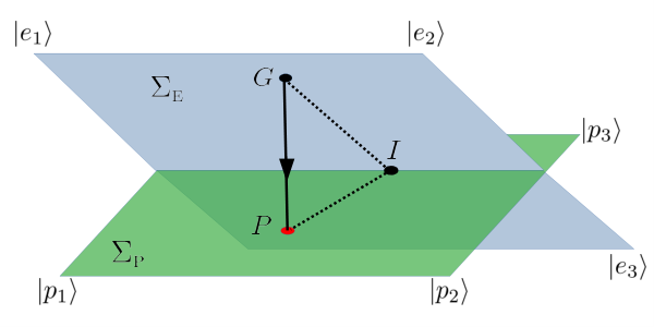
Figure 1 illustrates this proposition. Consider the convex hull $\Sigma_{\textsc{e}}=\left\{\rho=\sum_{i}Q_{i}\outerproduct{e_i}{e_i};\,Q_{i}\geq 0\wedge\sum_{i}Q_{i}=1\right\}$ in the Liouville space. The corners of the hull represent the pure states. Any density operator that is diagonal in the energy eigenbasis $\ket{e_i}$ is in $\Sigma_{\textsc{u}}$, including the Gibbs state ($G$ in Fig 1). Similarly, the convex hull $\Sigma_{\textsc{p}}=\left\{\rho=\sum_{i}P_{i}\outerproduct{p_i}{p_i};\,P_{i}\geq 0\wedge\sum_{i}P_{i}=1\right\}$ contains all possible density operators that are diagonal in the pointer basis $\ket{p_i}$. The density operators in the intersection of the two convex hulls are diagonal in both basis sets. A special point $I$ in the figure corresponds to $\rho=\frac{1}{d_{\textsc{s}}}I_{\textsc{s}}$ where $I_{\textsc{s}}$ is an identity operator and $d_{\textsc{s}}$ is the dimension of the system Hilbert space. The entropy of the system reaches its maximum value $\ln d_{\textsc{s}}$ at $I$. As the coupling gets stronger, the steady state deviates from the Gibbs state ($G$) toward the pointer limit ($P$) along the projection line ($\overline{GP}$). The projection line is “perpendicular” to $\Sigma_{\textsc{p}}$, meaning that the diagonal elements in the pointer basis are invariant along the projection line.

We justify the proposition by numerically investigating the exact dynamics of a simple spin-boson model. Following the standard open quantum system approach[2], we consider an isolated system consisting of a small subsystem $\mathcal{H}_{\textsc{s}}$ and environments $\mathcal{H}_{\textsc{b}}$. The unitary evolution of the total system follows the Liouville–von Neumann equation

where $H_{\textsc{b}}$ is the Hamiltonian of environment. For simplicity, we assume that the coupling Hamiltonian takes a bilinear form

where $X_{\ell}$ and $Y_{\ell}$ are operators in $\mathcal{H}_{\textsc{s}}$ and $\mathcal{H}_{\textsc{b}}$, respectively. Furthermore, we assume that $\commutator{X_k}{X_\ell}=0$ so that all $X_{\ell}$ share the same eigenkets $\ket{p_j}$ which we shall call pointer states. If there are degenerate subspaces, we choose a particular basis in the subspace such that the steady state becomes diagonal in the pointer basis.

The state of the system is represented by reduced density $\rho_{\textsc{s}}=\Tr_{\textsc{b}}\rho_{\textsc{sb}}$ which obeys the equation of motion

where we introduced a new operator,

Note that the time evolution of the system needs only limited information on the state of the environments through $\eta_{\ell}$.

In order to demonstrate the proposition, we consider a simple model consisting of a pair of identical qubits S₁ and S₂ whose Hamiltonian is given by

where $\sigma_{\ell}^{z,\pm},(\ell=1,2)$ are usual Pauli matrices for the $\ell$-th qubit, and $\omega_{0}$ and $\lambda_{\textsc{s}}$ the qubit excitation energy and the internal coupling strength, respectively. We write the energy eigenstates as $\ket{e_j},\,(j=1,\cdots,4)$ with eigenvalue $e_{j}$ starting from the ground state.

Each qubit S_ℓ is coupled to its own environment B_ℓ.¹¹ 1 If two qubits share the same environment, decoherence-free subspaces could be formed, which is protected from decoherence due to symmetry. We avoid the decoherence free subspace by using two independent environments. The environments are assumed to be ideal Bose gases whose Hamiltonians are given by $H_{\textsc{b}_{\ell}}=\sum_{k}\omega_{\ell}(k)\,a^{\dagger}_{\ell}(k)a_{\ell}(k)$, where $a^{\dagger}_{\ell}(k)$ and $a_{\ell}(k)$ are creation and annihilation operators for the $k$-th mode in $B_{\ell}$. The interaction Hamiltonian between S_ℓ and B_ℓ assumes a simple bilinear form $X_{\ell}\otimes Y_{\ell}$ where $X_{\ell}=\sigma^{x}_{\ell}$ and $Y_{\ell}=\sum_{k}\epsilon_{\ell}(k)\left[a^{\dagger}_{\ell}(k)+a_{\ell}(k)\right]$. The coupling strength between the system and the $k$-th mode in $B_{\ell}$ is denoted as $\epsilon_{\ell}(k)$.

The pointer states in this model are the simultaneous eigenkets of $X_{1}$ and $X_{2}$ and denoted as $\ket{p_1}=\ket{0\,0}$, $\ket{p_2}=\ket{0\,1}$, $\ket{p_3}=\ket{1\,0}$, and $\ket{p_4}=\ket{1\,1}$, where $\ket{0}$ and $\ket{1}$ are the eigenkets of $\sigma^{x}$.

When the coupling is weak, the stationary state is the Gibbs state

where $\rho^{\text{e}}_{jj}=e^{-\beta e_{j}}/\sum_{i}e^{-\beta e_{i}}$. Under the strong coupling limit, Proposition (1) claims that the stationary state density is given by

where $\rho^{p}_{jj}=\matrixelement{p_j}{\rho_\textsc{s}^\textsc{g}}{p_j}/Z_{\textsc{s}}$ can be explicitly expressed as

Now we show the transition from the Gibbs limit (7) to the pointer limit (8) by numerically solving Eq. (4). Assuming that the total system is initially in a product state $\rho(t_{0})=\rho_{\textsc{s}}(t_{0})\otimes\rho_{\textsc{b}}(t_{0})$ with the environment in a thermal state $\rho_{\textsc{b}}(t_{0})=\prod_{\ell}\exp(-\beta_\ell H_{\textsc{b}_\ell})/Z_{\textsc{b}_{\ell}}$, we obtain a formally exact expression of the system density in the interaction picture[23]

where the super operator $\mathscr{K}_{j}$ is defined by

with anti(+) and regular(-) commutators $\mathscr{S}^{\pm}_{\ell}=\commutator{X_\ell}{\cdot}_{\pm}$. The dissipation kernel $K^{\text{(d)}}_{\ell}(t)$ and noise kernel $K^{\text{(n)}}_{\ell}(t)$ are respectively the real and imaginary part of the correlation function $C_{\ell}(t)=\expectationvalue{Y_{\textsc{b}_\ell}(t) Y_{\textsc{b}_\ell}(t_0)}_{0}$ where the expectation value is taken with the initial environment state $\rho_{\textsc{b}_{\ell}}(t_{0})$. The time ordering operator $\overleftarrow{\mathscr{T}}$ in Eq. (10) chronologically orders the super operators $\mathscr{S}^{\pm}_{\ell}(t)$.

Kato and Tanimura[24, *Kato2016] showed that Eq (10) can be numerically evaluated if the spectral density of environments is of the Drude–Lorentz type:

where $\gamma_{\ell}$ and $\lambda_{\ell}$ are the response rate of environment and the overall coupling strength between qubit $S_{\ell}$ and environment $B_{\ell}$, respectively. Then, the environmental correlation can be expressed with reasonable accuracy as[26]

where $c_{\ell}=2/\beta_{\ell}-\gamma_{\ell}\Delta_{\ell}-i\gamma_{\ell}$ and $\Delta_{\ell}=\gamma_{\ell}\beta_{\ell}/6$.

Following Kato and Tanimura[24, 25], we introduce a set of auxiliary operators

where

Index $n_{\ell}$ associated with environment $B_{\ell}$ runs from 0 through infinity. Only the first three lowest order auxiliary operators are needed for $\rho_{\textsc{s}}(t)=\zeta_{0,0}(t)$, $\eta_{1}=\lambda_{1}\left[\zeta_{1,0}(t)-i\Delta_{1}\mathscr{S}^{-}_{1}(t)\zeta_{0,0}(t)\right]$ and $\eta_{2}=\lambda_{2}\left[\zeta_{0,1}(t)-i\Delta_{2}\mathscr{S}^{-}_{2}(t)\zeta_{0,0}(t)\right]$. However, the dynamics of auxiliary operators is determined by an infinite set of coupled ODEs or so-called hierarchical equations of motion[24, 25]

with the initial condition $\zeta_{n_{1},n_{2}}(t_{0})=0$ except for $\zeta_{0,0}(t_{0})=\rho_{\textsc{s}}(t_{0})$. The infinite hierarchy is truncated at depth $d=50$ such that higher depth auxiliary operators do not significantly contribute to the first two depths.

First, we investigate the equilibrium situation where the initial states of the two environments are identical ($\lambda_{1}=\lambda_{2}\equiv\lambda_{\textsc{b}}$, $T_{1}=T_{2}\equiv T$, $\gamma_{1}=\gamma_{2}\equiv\gamma$). We tried more than ten different initial densities, and all converged to the same stationary state. In Fig. 2, the matrix elements of the stationary state density are plotted as a function of the coupling strength $\lambda_{\textsc{b}}$ using the energy eigenbasis and the pointer basis. The density matrix in the energy eigenbasis shows that the Gibbs state is realized only at the weak coupling limit. The diagonal elements deviate from the Gibbs state as the coupling increases. The off-diagonal elements indicate that the superposition of eigenstates $\ket{e_1}$ and $\ket{e_4}$ grows rapidly and thus decoherence does not fully take place in the energy eigenbasis. Both the diagonal and off-diagonal elements approach the pointer limit predicted by Eq. (8).

When the matrix elements of the same density operator are evaluated in the pointer basis, all of the off-diagonal elements tend to vanish as the coupling strength increases, suggesting that full decoherence takes place in the pointer basis. The diagonal elements are remarkably insensitive to the coupling strength and in good agreement with Eq. (9) regardless of the coupling strength. The invariance of the diagonal elements confirms that the projection is perpendicular to the convex hull $\Sigma_{\textsc{p}}$. (See Fig. 1.) In Fig. 3 the deviation of the steady state from the Gibbs state and its approach to the pointer limit are measured by fidelity $F(\rho,\rho^{\prime})=\left(\tr\{\sqrt{\rho}\,\rho^{\prime}\sqrt{\rho}\}\right)^{2}$. At $\lambda_{\textsc{b}}=4$, the distance between the steady state and the pointer limit nearly vanishes.

Through the continuous measurement, the environments gain information of the system and the system loses information. Accordingly, the entropy of the system increases.[18, 27] As the coupling gets stronger, more information is expected to be lost and thus the entropy goes up monotonically. Figure 3 confirms the increase of the von Neumann entropy which converges to the pointer limit (8) at the strong coupling limit.

As further evidence of continuous measurement by environments, we also investigated a non-equilibrium steady state. When different temperatures are used, heat flows through the system. Heat from the environment B_ℓ to the system can be computed as

Figure 4 shows the steady state heat current as a function of the coupling strength. In the weak coupling regime, the current increases linearly as expected from the linear response theory. However, the heat current reaches its maximum and dies off rather quickly as the coupling becomes stronger. This suppression of heat is predicted earlier as a consequence of the quantum zeno effect[28] based on a heuristic argument and is observed by Kato-Tanimura[24].

The present results show that indeed the decoherence due to environments is responsible for the suppression of heat. The off-diagonal elements of the steady state density look almost identical to those in the stationary state at a single effective temperature $T=(T_{1}+T_{2})/2$ However, there is small but significant difference where the heat current is strong. The elements $\rho_{13}$ and $\rho_{24}$ deviate from $\rho_{12}$ and $\rho_{34}$ due to the difference in decoherence power between the two environments. In general a higher temperature environment causes stronger decoherence.[29] However, it also depends on the coupling strength as well. When the coupling strength overcomes the asymmetry in temperature, the decoherence power of the two environments becomes nearly identical and eventually the asymmetry in the off-diagonal element responsible for the heat conduction vanishes.

In conclusion, we claim that the “thermal equilibrium” of a small quantum system is not the Gibbs state when the coupling to the environments is strong. Due to continuous measurement by the environment, the stationary state loses the coherency between the pointer states and thus the density is diagonal in the pointer basis rather than in the energy eigenbasis. We further claim that the the stationary state density at the strong coupling limit is the Gibbs state projected onto the pointer basis. The diagonal elements in the pointer basis appear to be insensitive to the coupling strength. We have demonstrated this proposition by exact numerical calculation using the hierarchical equations of motion. This strong coupling limit can be used as a bench mark test for analytic models such as the Hamiltonian of mean force.