跳到论文正文
W Papers独立论文阅读器 arXiv:1712.08685 论文正文 计算阅读时间 · 0%
引用这篇论文根据当前论文元数据生成,正式投稿前建议核对。


License: arXiv.org perpetual non-exclusive license
arXiv:1712.08685v2 [cs.SI] 08 May 2018

Sampling for Approximate Bipartite Network Projection

Nesreen K. Ahmed Nick Duffield Liangzhen Xia Intel Labs, CA Texas A&M University Texas A&M University nesreen.k.ahmed@intel.com duffieldng@tamu.edu xialiangzhen1226@gmail.com
Abstract

Bipartite networks manifest as a stream of edges that represent transactions, e.g., purchases by retail customers. Many machine learning applications employ neighborhood-based measures to characterize the similarity among the nodes, such as the pairwise number of common neighbors (CN) and related metrics. While the number of node pairs that share neighbors is potentially enormous, only a relatively small proportion of them have many common neighbors. This motivates finding a weighted sampling approach to preferentially sample these node pairs. This paper presents a new sampling algorithm that provides a fixed size unbiased estimate of the similarity matrix resulting from a bipartite graph stream projection. The algorithm has two components. First, it maintains a reservoir of sampled bipartite edges with sampling weights that favor selection of high similarity nodes. Second, arriving edges generate a stream of similarity updates based on their adjacency with the current sample. These updates are aggregated in a second reservoir sample-based stream aggregator to yield the final unbiased estimate. Experiments on real world graphs show that a 10% sample at each stage yields estimates of high similarity edges with weighted relative errors of about 1​0−2\mathchar 28721\mathchar 28720^{\mathchar 8704\mathchar 28722}.

1 Introduction

Networks arise as a natural representation for data, where nodes represent people/objects and edges represent the relationships among them. The recent years have witnessed a tremendous amount of research devoted to the analysis and modeling of complex networks Liben-Nowell and Kleinberg (2007). Bipartite networks are a special class of networks represented as a graph G=(U,V,K)\mathchar 28999\mathchar 12349\delimiter 67273472\mathchar 29013\mathchar 24891\mathchar 29014\mathchar 24891\mathchar 29003\delimiter 84054785, whose nodes divide into two sets U\mathchar 29013 and V\mathchar 29014, with edges allowed only between two nodes that belong to different sets, i.e., (u,|)∈K\delimiter 67273472\mathchar 29045\mathchar 24891\delimiter 69640972\delimiter 84054785\mathchar 12850\mathchar 29003 is an edge, only if u∈U\mathchar 29045\mathchar 12850\mathchar 29013 and |∈V\delimiter 69640972\mathchar 12850\mathchar 29014. Thus, bipartite networks represent relationships between two different types of nodes. Bipartite networks are a natural model for many systems and applications. For example, bipartite networks are used to model the relationships between users/customers and the products/services they consume. General examples include collaboration networks in which actors are connected by a common collaboration act (e.g., author-paper, actor-movie) and opinion networks in which users are connected by shared objects (e.g., user-product, user-movie, reader-book). Clearly, a bipartite network manifests as a stream of edges representing the transactions between two types of nodes over time, e.g., retail customers purchasing products daily. Moreover, these dynamic bipartite networks are usually large, due to the prolific amount of activity carrying a wealth of useful behavioral data for business analytics.

While the bipartite representation is indeed useful by itself, many applications focus on analyzing the relationships among a particular set of nodes Zhou et al. (2007). For the convenience of these applications, a bipartite network is usually compressed by using a one-mode projection (i.e., projection on one set of the nodes), this is called bipartite network projection. For example, for a one-mode projection on U\mathchar 29013, the projected graph will contain only U\mathchar 29013-nodes and two nodes u,u′∈U\mathchar 29045\mathchar 24891\mathchar 29045^{\mathchar 560}\mathchar 12850\mathchar 29013 are connected if there is at least one common neighbor |∈V\delimiter 69640972\mathchar 12850\mathchar 29014, such that (u,|)∈K\delimiter 67273472\mathchar 29045\mathchar 24891\delimiter 69640972\delimiter 84054785\mathchar 12850\mathchar 29003 and (u′,|)∈K\delimiter 67273472\mathchar 29045^{\mathchar 560}\mathchar 24891\delimiter 69640972\delimiter 84054785\mathchar 12850\mathchar 29003. This results in the U\mathchar 29013-projection graph GU=(U,KU,C)\mathchar 28999_{\mathchar 29013}\mathchar 12349\delimiter 67273472\mathchar 29013\mathchar 24891\mathchar 29003_{\mathchar 29013}\mathchar 24891\mathchar 28995\delimiter 84054785 which is a weighted graph characterized by the set of nodes U\mathchar 29013, and the edges among them KU\mathchar 29003_{\mathchar 29013}. The matrix C={C⁡(u,u′)}U×U\mathchar 28995\mathchar 12349\{\mathchar 28995{\delimiter 67273472\mathchar 29045\mathchar 24891\mathchar 29045^{\mathchar 560}\delimiter 84054785}\}_{\mathchar 29013\mathchar 8706\mathchar 29013} represents the weighted adjacency matrix for the U\mathchar 29013-projection graph, where the weight C⁡(u,u′)\mathchar 28995{\delimiter 67273472\mathchar 29045\mathchar 24891\mathchar 29045^{\mathchar 560}\delimiter 84054785} represents the strength of the similarity between the two nodes u,u′∈U\mathchar 29045\mathchar 24891\mathchar 29045^{\mathchar 560}\mathchar 12850\mathchar 29013.

How to weight the edges has been a key question in one-mode projections and their applications. Several weighting functions were proposed. For example, neighborhood-based methods Ning et al. (2015); Zhou et al. (2007) measure the similarity between two nodes proportional to the overlap of their neighbor sets. Another example in Fouss et al. (2007) uses random walks to measure the similarity between nodes. Finding similar nodes (e.g., users, objects, items) in a graph is a fundamental problem with applications in recommender systems Koren (2008), collaborative filtering Herlocker et al. (2004), social link prediction Liben-Nowell and Kleinberg (2007), text analysis Salton et al. (1993), among others.

Motivated by these applications, we study the bipartite network projection problem in the streaming computational model Muthukrishnan (2005). Thus, given a bipartite network whose edges arrive as a stream in some arbitrary order, we compute the projection graph (i.e., weighted matrix C\mathchar 28995) as the stream is progressing. In this paper, we focus on the common neighbors approach as the weight function. The common neighbors weight is defined for any two nodes u,u′∈U\mathchar 29045\mathchar 24891\mathchar 29045^{\mathchar 560}\mathchar 12850\mathchar 29013, as the size of the intersection of their neighborhood sets Γ⁡(u)\mathchar 28672\delimiter 67273472\mathchar 29045\delimiter 84054785 and Γ⁡(u′)\mathchar 28672\delimiter 67273472\mathchar 29045^{\mathchar 560}\delimiter 84054785, where Γ⁡(u)⊂V\mathchar 28672\delimiter 67273472\mathchar 29045\delimiter 84054785\mathchar 12826\mathchar 29014 is the set of neighbors of u\mathchar 29045. Thus, their projected weight is C⁡(u,u′)=|Γ⁡(u)∩Γ⁡(u′)|\mathchar 28995\delimiter 67273472\mathchar 29045\mathchar 24891\mathchar 29045^{\mathchar 560}\delimiter 84054785\mathchar 12349\delimiter 69640972\mathchar 28672\delimiter 67273472\mathchar 29045\delimiter 84054785\mathchar 8796\mathchar 28672\delimiter 67273472\mathchar 29045^{\mathchar 560}\delimiter 84054785\delimiter 69640972. It is convenient to think of a bipartite network as a (binary) matrix A∈ℝU×V\mathchar 28993\mathchar 12850\mathbb{\mathchar 29010}^{\mathchar 29013\mathchar 8706\mathchar 29014}, where the rows represent the node set U\mathchar 29013, and the columns represent the node set V\mathchar 29014. In this case, computing the U\mathchar 29013-projection matrix using common neighbors is equivalent to C=A​A⊺\mathchar 28995\mathchar 12349\mathchar 28993\mathchar 28993^{\intercal}, where C∈ℝU×U\mathchar 28995\mathchar 12850\mathbb{\mathchar 29010}^{\mathchar 29013\mathchar 8706\mathchar 29013}. In addition, the common neighbors is a fundamental component in many weighing functions (e.g., cosine similarity), such as those used in collaborative filtering.

The naive solution for this problem is to compute C=A​A⊺\mathchar 28995\mathchar 12349\mathchar 28993\mathchar 28993^{\intercal} exhaustively with 𝒪⁡(|U|2)\mathcal{\mathchar 29007}\delimiter 67273472\delimiter 69640972\mathchar 29013\delimiter 69640972^{\mathchar 28722}\delimiter 84054785 for space and time complexity. However, this is unfeasible for streaming/large bipartite networks Muthukrishnan (2005); Ahmed et al. (2014b). Instead, given a streaming bipartite network (whose edges arrive over time), our goal is to compute a sample of the projection graph that contains an unbiased estimate of the largest entries in the projection matrix C\mathchar 28995.

Contributions. Our main contribution is a novel single-pass, adaptive, weighted sampling scheme in fixed storage for approximate bipartite projection in streaming bipartite networks. Our approach has three steps. First, we maintain a weighted edge sample from the streaming bipartite graph. Second, we observe that the number of common neighbors C⁡(u,u′)\mathchar 28995\delimiter 67273472\mathchar 29045\mathchar 24891\mathchar 29045^{\mathchar 560}\delimiter 84054785 between two vertices u\mathchar 29045 and u′∈U\mathchar 29045^{\mathchar 560}\mathchar 12850\mathchar 29013 is equal to the number of wedges (u,|,u′)\delimiter 67273472\mathchar 29045\mathchar 24891\delimiter 69640972\mathchar 24891\mathchar 29045^{\mathchar 560}\delimiter 84054785 connecting them, where (u,|)∈K\delimiter 67273472\mathchar 29045\mathchar 24891\delimiter 69640972\delimiter 84054785\mathchar 12850\mathchar 29003 and (u′,|)∈K\delimiter 67273472\mathchar 29045^{\mathchar 560}\mathchar 24891\delimiter 69640972\delimiter 84054785\mathchar 12850\mathchar 29003 for some |∈V\delimiter 69640972\mathchar 12850\mathchar 29014. Thus, each bipartite edge arriving to the sample generates unbiased estimators of updates to the similarity matrix through the wedges it creates. Third, a further sample-based aggregation accumulates estimates of the projection graph in fixed-size storage.

2 Framework

Problem Definition and Key Intuition. Let G=(U,V,K)\mathchar 28999\mathchar 12349\delimiter 67273472\mathchar 29013\mathchar 24891\mathchar 29014\mathchar 24891\mathchar 29003\delimiter 84054785 be a bipartite graph, and Γ(u)={|:(u,|)∈K}\mathchar 28672\delimiter 67273472\mathchar 29045\delimiter 84054785\mathchar 12349\{\delimiter 69640972\mathchar 12346\delimiter 67273472\mathchar 29045\mathchar 24891\delimiter 69640972\delimiter 84054785\mathchar 12850\mathchar 29003\} denote the set of neighbors of u∈U\mathchar 29045\mathchar 12850\mathchar 29013. We study the problem of bipartite network projection in data streams, where G\mathchar 28999 is compressed by using a one-mode projection. Thus, for a one-mode projection on U\mathchar 29013, the projected graph will contain only U\mathchar 29013-nodes and two nodes u,u′∈U\mathchar 29045\mathchar 24891\mathchar 29045^{\mathchar 560}\mathchar 12850\mathchar 29013 are connected if there is at least one common neighbor |∈V\delimiter 69640972\mathchar 12850\mathchar 29014, such that (u,|)∈K\delimiter 67273472\mathchar 29045\mathchar 24891\delimiter 69640972\delimiter 84054785\mathchar 12850\mathchar 29003 and (u′,|)∈K\delimiter 67273472\mathchar 29045^{\mathchar 560}\mathchar 24891\delimiter 69640972\delimiter 84054785\mathchar 12850\mathchar 29003. This results in the U\mathchar 29013-projection graph GU=(U,KU,C)\mathchar 28999_{\mathchar 29013}\mathchar 12349\delimiter 67273472\mathchar 29013\mathchar 24891\mathchar 29003_{\mathchar 29013}\mathchar 24891\mathchar 28995\delimiter 84054785 which is a weighted graph characterized by the set of nodes U\mathchar 29013, and the edges among them KU\mathchar 29003_{\mathchar 29013}. The matrix C={C⁡(u,u′)}U×U\mathchar 28995\mathchar 12349\{\mathchar 28995\delimiter 67273472\mathchar 29045\mathchar 24891\mathchar 29045^{\mathchar 560}\delimiter 84054785\}_{\mathchar 29013\mathchar 8706\mathchar 29013} represents the weighted adjacency matrix for the U\mathchar 29013-projection graph, where the weight C⁡(u,u′)\mathchar 28995\delimiter 67273472\mathchar 29045\mathchar 24891\mathchar 29045^{\mathchar 560}\delimiter 84054785 represents the strength of the similarity between any two nodes u,u′∈U\mathchar 29045\mathchar 24891\mathchar 29045^{\mathchar 560}\mathchar 12850\mathchar 29013. In this paper, we propose a novel approximation framework based on sampling to avoid the direct computation of all pairs in C\mathchar 28995.

Definition 1 (Approximate Bipartite Projection).

Given a bipartite network G=(U,V,K)\mathchar 28999\mathchar 12349\delimiter 67273472\mathchar 29013\mathchar 24891\mathchar 29014\mathchar 24891\mathchar 29003\delimiter 84054785 with (binary) adjacency matrix A∈ℝU×V\mathchar 28993\mathchar 12850\mathbb{\mathchar 29010}^{\mathchar 29013\mathchar 8706\mathchar 29014}: find the vertex pair (u,u′)∈U×U\delimiter 67273472\mathchar 29045\mathchar 24891\mathchar 29045^{\mathchar 560}\delimiter 84054785\mathchar 12850\mathchar 29013\mathchar 8706\mathchar 29013 that maximizes C=A​A⊺\mathchar 28995\mathchar 12349\mathchar 28993\mathchar 28993^{\intercal}. More generally, assume a given parameter k\mathchar 29035, find the k\mathchar 29035 vertex pairs {(u1,u1′),…,(uk,uk′)}\{\delimiter 67273472\mathchar 29045_{\mathchar 28721}\mathchar 24891\mathchar 29045^{\mathchar 560}_{\mathchar 28721}\delimiter 84054785\mathchar 24891\dots\mathchar 24891\delimiter 67273472\mathchar 29045_{\mathchar 29035}\mathchar 24891\mathchar 29045^{\mathchar 560}_{\mathchar 29035}\delimiter 84054785\} corresponding to the k\mathchar 29035 largest entries in C\mathchar 28995.

Note that Definition 1 corresponds to finding the pairs with largest number of common neighbors. Intuitively, the number of common neighbors C⁡(u,u′)\mathchar 28995\delimiter 67273472\mathchar 29045\mathchar 24891\mathchar 29045^{\mathchar 560}\delimiter 84054785 between two vertices u,u′∈U\mathchar 29045\mathchar 24891\mathchar 29045^{\mathchar 560}\mathchar 12850\mathchar 29013, is equivalent to the number of wedges (u,|,u′)\delimiter 67273472\mathchar 29045\mathchar 24891\delimiter 69640972\mathchar 24891\mathchar 29045^{\mathchar 560}\delimiter 84054785 connecting them, where (u,|)∈K\delimiter 67273472\mathchar 29045\mathchar 24891\delimiter 69640972\delimiter 84054785\mathchar 12850\mathchar 29003 and (u′,|)∈K\delimiter 67273472\mathchar 29045^{\mathchar 560}\mathchar 24891\delimiter 69640972\delimiter 84054785\mathchar 12850\mathchar 29003 for some |∈V\delimiter 69640972\mathchar 12850\mathchar 29014.

Streaming Bipartite Network Projection. Bipartite networks are used to model dynamically evolving transactions represented as a stream of edges between two types of nodes over time. In the streaming bipartite graph model, edges K\mathchar 29003 arrive in some arbitrary order {ei:i∈[|K|]}\{\mathchar 29029_{\mathchar 29033}\mathchar 12346\mathchar 29033\mathchar 12850\delimiter 67482370\delimiter 69640972\mathchar 29003\delimiter 69640972\delimiter 84267779\}. Let Kt={ei:i∈[t]}\mathchar 29003_{\mathchar 29044}\mathchar 12349\{\mathchar 29029_{\mathchar 29033}\mathchar 12346\mathchar 29033\mathchar 12850\delimiter 67482370\mathchar 29044\delimiter 84267779\} denote the first t\mathchar 29044 arriving edges, Gt=(Ut,Vt,Kt)\mathchar 28999_{\mathchar 29044}\mathchar 12349\delimiter 67273472\mathchar 29013_{\mathchar 29044}\mathchar 24891\mathchar 29014_{\mathchar 29044}\mathchar 24891\mathchar 29003_{\mathchar 29044}\delimiter 84054785 the bipartite graph induced by the first t\mathchar 29044 arriving edges, and Ct\mathchar 28995_{\mathchar 29044} the corresponding similarity matrix. We aim to estimate the largest entries of Ct\mathchar 28995_{\mathchar 29044} for any t\mathchar 29044.

2.1 Adaptive Bipartite Graph Sampling

We construct a weighted fixed-size reservoir sample of bipartite edges in which edge weights dynamically adapt to their topological importance (i.e., priority). For a reservoir of size m\mathchar 29037, we admit the first m\mathchar 29037 edges, while for t>m\mathchar 29044\mathchar 12606\mathchar 29037, the sample set comprises a subset K^t≤Kt\widehat{\mathchar 29003}_{\mathchar 29044}\mathchar 12820\mathchar 29003_{\mathchar 29044} of the first t\mathchar 29044 arriving edges, with fixed size |K^t|=m\delimiter 69640972\widehat{\mathchar 29003}_{\mathchar 29044}\delimiter 69640972\mathchar 12349\mathchar 29037 for each t≥m\mathchar 29044\mathchar 12821\mathchar 29037. This is achieved by provisionally admitting the arriving edge at each t>m\mathchar 29044\mathchar 12606\mathchar 29037 to the reservoir, then discarding one of the resulting m+1\mathchar 29037\mathchar 8235\mathchar 28721 edges by the random mechanism that we now describe.

Since edges are assumed unique, each edge ei\mathchar 29029_{\mathchar 29033} is identified with its the arrival order i∈[|K|]\mathchar 29033\mathchar 12850\delimiter 67482370\delimiter 69640972\mathchar 29003\delimiter 69640972\delimiter 84267779. All sampling outcomes are determined by independent random variables βi\mathchar 28940_{\mathchar 29033}, uniformly distributed in (0,1]\delimiter 67273472\mathchar 28720\mathchar 24891\mathchar 28721\delimiter 84267779, assigned to each edge i\mathchar 29033 on arrival. Any edge present in the sample at time t≥i\mathchar 29044\mathchar 12821\mathchar 29033 possess a weight wi,t\mathchar 29047_{\mathchar 29033\mathchar 24891\mathchar 29044} whose form is described in Section 2.2. The priority of i\mathchar 29033 at time t\mathchar 29044 is defined as ri,t=wi,t/βi\mathchar 29042_{\mathchar 29033\mathchar 24891\mathchar 29044}\mathchar 12349\mathchar 29047_{\mathchar 29033\mathchar 24891\mathchar 29044}\delimiter 68408078\mathchar 28940_{\mathchar 29033}. Edge i\mathchar 29033 is provisionally admitted to the reservoir forming the set K^i′=K^i−1∪{i}\widehat{\mathchar 29003}^{\mathchar 560}_{\mathchar 29033}\mathchar 12349\widehat{\mathchar 29003}_{\mathchar 29033\mathchar 8704\mathchar 28721}\mathchar 8795\{\mathchar 29033\}, from which we then discard the edge with minimal priority, whose value is called the threshold.

Theorem 1 below establishes unbiased estimators of edge counts. Define the edge indicator Si,t\mathchar 29011_{\mathchar 29033\mathchar 24891\mathchar 29044} taking the value 1\mathchar 28721 if t≥i\mathchar 29044\mathchar 12821\mathchar 29033 and 0\mathchar 28720 otherwise. We will construct inverse probability edge estimators S^i,t=I⁡(i∈K^t)/qi,t\widehat{\mathchar 29011}_{\mathchar 29033\mathchar 24891\mathchar 29044}\mathchar 12349\mathchar 29001\delimiter 67273472\mathchar 29033\mathchar 12850\widehat{\mathchar 29003}_{\mathchar 29044}\delimiter 84054785\delimiter 68408078\mathchar 29041_{\mathchar 29033\mathchar 24891\mathchar 29044} of Si,t\mathchar 29011_{\mathchar 29033\mathchar 24891\mathchar 29044} and prove they are unbiased. This entails showing that qi,t=min⁡{1,mini≤s≤t⁡wi,s/zs}\mathchar 29041_{\mathchar 29033\mathchar 24891\mathchar 29044}\mathchar 12349\min\{\mathchar 28721\mathchar 24891\min_{\mathchar 29033\mathchar 12820\mathchar 29043\mathchar 12820\mathchar 29044}\mathchar 29047_{\mathchar 29033\mathchar 24891\mathchar 29043}\delimiter 68408078\mathchar 29050_{\mathchar 29043}\} is the probability that i∈Kt\mathchar 29033\mathchar 12850\mathchar 29003_{\mathchar 29044}, conditional on the set 𝒵i,t={zi,…,zt}{\mathcal{\mathchar 29018}}_{\mathchar 29033\mathchar 24891\mathchar 29044}\mathchar 12349\{\mathchar 29050_{\mathchar 29033}\mathchar 24891\ldots\mathchar 24891\mathchar 29050_{\mathchar 29044}\} of thresholds zs=minj∈K^s′⁡rj,s\mathchar 29050_{\mathchar 29043}\mathchar 12349\min_{\mathchar 29034\mathchar 12850\widehat{\mathchar 29003}^{\mathchar 560}_{\mathchar 29043}}\mathchar 29042_{\mathchar 29034\mathchar 24891\mathchar 29043} since its arrival.

Theorem 1.

S^i,t\widehat{\mathchar 29011}_{\mathchar 29033\mathchar 24891\mathchar 29044} is an unbiased estimator of Si,t\mathchar 29011_{\mathchar 29033\mathchar 24891\mathchar 29044}.

Proof.

Trivially S^i,t=0=Si,t\widehat{\mathchar 29011}_{\mathchar 29033\mathchar 24891\mathchar 29044}\mathchar 12349\mathchar 28720\mathchar 12349\mathchar 29011_{\mathchar 29033\mathchar 24891\mathchar 29044} for t<i\mathchar 29044\mathchar 12604\mathchar 29033. For t≥i\mathchar 29044\mathchar 12821\mathchar 29033 let zi,t=minj∈K^t\{i}⁡rj,t\mathchar 29050_{\mathchar 29033\mathchar 24891\mathchar 29044}\mathchar 12349\min_{\mathchar 29034\mathchar 12850\widehat{\mathchar 29003}_{\mathchar 29044}\mathchar 8814\{\mathchar 29033\}}\mathchar 29042_{\mathchar 29034\mathchar 24891\mathchar 29044}. Observe i∈K^t\mathchar 29033\mathchar 12850\widehat{\mathchar 29003}_{\mathchar 29044} iff ri,s\mathchar 29042_{\mathchar 29033\mathchar 24891\mathchar 29043} is not the smallest priority in any K^s′\widehat{\mathchar 29003}^{\mathchar 560}_{\mathchar 29043} for all s∈[i,t]\mathchar 29043\mathchar 12850\delimiter 67482370\mathchar 29033\mathchar 24891\mathchar 29044\delimiter 84267779. In other words

{i∈K^t}=∩s∈[i,t]{wi,sUNKNOWNi>zi,s}={βi<mins∈[i,t]wi,szi,s}\{\mathchar 29033\mathchar 12850\widehat{\mathchar 29003}_{\mathchar 29044}\}\mathchar 12349\mathchar 8796_{\mathchar 29043\mathchar 12850\delimiter 67482370\mathchar 29033\mathchar 24891\mathchar 29044\delimiter 84267779}\{{{\mathchar 29047_{\mathchar 29033\mathchar 24891\mathchar 29043}\over\mathchar 28940_{\mathchar 29033}}}\mathchar 12606\mathchar 29050_{\mathchar 29033\mathchar 24891\mathchar 29043}\}\\ \mathchar 12349\{\mathchar 28940_{\mathchar 29033}\mathchar 12604\min_{\mathchar 29043\mathchar 12850\delimiter 67482370\mathchar 29033\mathchar 24891\mathchar 29044\delimiter 84267779}{{\mathchar 29047_{\mathchar 29033\mathchar 24891\mathchar 29043}\over\mathchar 29050_{\mathchar 29033\mathchar 24891\mathchar 29043}}}\}

Thus ℙ⁡[i∈K^t|𝒵i,t]=q~i,t:=min⁡{1,mins∈[i,t]⁡wi,s/zi,s}{\mathbb{\mathchar 29008}}\delimiter 67482370\mathchar 29033\mathchar 12850\widehat{\mathchar 29003}_{\mathchar 29044}\delimiter 69640972{\mathcal{\mathchar 29018}}_{\mathchar 29033\mathchar 24891\mathchar 29044}\delimiter 84267779\mathchar 12349\tilde{\mathchar 29041}_{\mathchar 29033\mathchar 24891\mathchar 29044}\mathchar 12346\mathchar 12349\min\{\mathchar 28721\mathchar 24891\min_{\mathchar 29043\mathchar 12850\delimiter 67482370\mathchar 29033\mathchar 24891\mathchar 29044\delimiter 84267779}\mathchar 29047_{\mathchar 29033\mathchar 24891\mathchar 29043}\delimiter 68408078\mathchar 29050_{\mathchar 29033\mathchar 24891\mathchar 29043}\}. Note that q~i,t=qi,t\tilde{\mathchar 29041}_{\mathchar 29033\mathchar 24891\mathchar 29044}\mathchar 12349\mathchar 29041_{\mathchar 29033\mathchar 24891\mathchar 29044} when i∈K^t\mathchar 29033\mathchar 12850\widehat{\mathchar 29003}_{\mathchar 29044} since then zi,s=zs\mathchar 29050_{\mathchar 29033\mathchar 24891\mathchar 29043}\mathchar 12349\mathchar 29050_{\mathchar 29043} for all s∈[i,t]\mathchar 29043\mathchar 12850\delimiter 67482370\mathchar 29033\mathchar 24891\mathchar 29044\delimiter 84267779. Hence when t≥i\mathchar 29044\mathchar 12821\mathchar 29033

𝔼⁡[S^i,t|𝒵i,t]=ℙ⁡[I⁡(i∈K^t)|𝒵i,t]/q~i,t=1=Si,t{\mathbb{\mathchar 28997}}\delimiter 67482370\widehat{\mathchar 29011}_{\mathchar 29033\mathchar 24891\mathchar 29044}\delimiter 69640972{\mathcal{\mathchar 29018}}_{\mathchar 29033\mathchar 24891\mathchar 29044}\delimiter 84267779\mathchar 12349{{\mathbb{\mathchar 29008}}\delimiter 67482370\mathchar 29001\delimiter 67273472\mathchar 29033\mathchar 12850\widehat{\mathchar 29003}_{\mathchar 29044}\delimiter 84054785\delimiter 69640972{\mathcal{\mathchar 29018}}_{\mathchar 29033\mathchar 24891\mathchar 29044}\delimiter 84267779}\delimiter 68408078{\tilde{\mathchar 29041}_{\mathchar 29033\mathchar 24891\mathchar 29044}}\mathchar 12349\mathchar 28721\mathchar 12349\mathchar 29011_{\mathchar 29033\mathchar 24891\mathchar 29044} (1)

independent of 𝒵i,t{\mathcal{\mathchar 29018}}_{\mathchar 29033\mathchar 24891\mathchar 29044} and hence 𝔼⁡[S^i,t]=Si,t{\mathbb{\mathchar 28997}}\delimiter 67482370\widehat{\mathchar 29011}_{\mathchar 29033\mathchar 24891\mathchar 29044}\delimiter 84267779\mathchar 12349\mathchar 29011_{\mathchar 29033\mathchar 24891\mathchar 29044}. ∎

Let zt∗=max⁡𝒵m,t\mathchar 29050^{\mathchar 8707}_{\mathchar 29044}\mathchar 12349\max{\mathcal{\mathchar 29018}}_{\mathchar 29037\mathchar 24891\mathchar 29044}. Theorem 2 shows that pi,t=min⁡{1,mini≤s≤t⁡wi,szs∗}\mathchar 29040_{\mathchar 29033\mathchar 24891\mathchar 29044}\mathchar 12349\min\{\mathchar 28721\mathchar 24891\min_{\mathchar 29033\mathchar 12820\mathchar 29043\mathchar 12820\mathchar 29044}{{\mathchar 29047_{\mathchar 29033\mathchar 24891\mathchar 29043}\over\mathchar 29050^{\mathchar 8707}_{\mathchar 29043}}}\} can be used in place of qi,t\mathchar 29041_{\mathchar 29033\mathchar 24891\mathchar 29044}. This simplifies computation since: (a) each pi,t\mathchar 29040_{\mathchar 29033\mathchar 24891\mathchar 29044} uses the same zt∗\mathchar 29050^{\mathchar 8707}_{\mathchar 29044}; (b) updates of pi,t\mathchar 29040_{\mathchar 29033\mathchar 24891\mathchar 29044} can be deferred until times t\mathchar 29044 at which wi,t\mathchar 29047_{\mathchar 29033\mathchar 24891\mathchar 29044} increases.

Theorem 2.

If t→wi,t\mathchar 29044\mathchar 12833\mathchar 29047_{\mathchar 29033\mathchar 24891\mathchar 29044} is non-decreasing for each i\mathchar 29033 then qi,t=pi,t\mathchar 29041_{\mathchar 29033\mathchar 24891\mathchar 29044}\mathchar 12349\mathchar 29040_{\mathchar 29033\mathchar 24891\mathchar 29044} and hence S^i,t=I⁡(i∈K^t)/pi,t\widehat{\mathchar 29011}_{\mathchar 29033\mathchar 24891\mathchar 29044}\mathchar 12349\mathchar 29001\delimiter 67273472\mathchar 29033\mathchar 12850\widehat{\mathchar 29003}_{\mathchar 29044}\delimiter 84054785\delimiter 68408078\mathchar 29040_{\mathchar 29033\mathchar 24891\mathchar 29044} for all t≥i\mathchar 29044\mathchar 12821\mathchar 29033.

Proof.

Let dt\mathchar 29028_{\mathchar 29044} denote the edge discarded during processing arrival t\mathchar 29044. By assumption, i\mathchar 29033 is admitted to K^i\widehat{\mathchar 29003}_{\mathchar 29033} and since wj,t\mathchar 29047_{\mathchar 29034\mathchar 24891\mathchar 29044} is non-decreasing in t\mathchar 29044, zi=zi,i=wdi,i/βdi≥wdi,s/βdi>zs\mathchar 29050_{\mathchar 29033}\mathchar 12349\mathchar 29050_{\mathchar 29033\mathchar 24891\mathchar 29033}\mathchar 12349\mathchar 29047_{\mathchar 29028_{\mathchar 29033}\mathchar 24891\mathchar 29033}\delimiter 68408078\mathchar 28940_{\mathchar 29028_{\mathchar 29033}}\mathchar 12821\mathchar 29047_{\mathchar 29028_{\mathchar 29033}\mathchar 24891\mathchar 29043}\delimiter 68408078\mathchar 28940_{\mathchar 29028_{\mathchar 29033}}\mathchar 12606\mathchar 29050_{\mathchar 29043} for all s∈[di,i]\mathchar 29043\mathchar 12850\delimiter 67482370\mathchar 29028_{\mathchar 29033}\mathchar 24891\mathchar 29033\delimiter 84267779 in order that di∈Ks\mathchar 29028_{\mathchar 29033}\mathchar 12850\mathchar 29003_{\mathchar 29043} for all s∈[di,i−1]\mathchar 29043\mathchar 12850\delimiter 67482370\mathchar 29028_{\mathchar 29033}\mathchar 24891\mathchar 29033\mathchar 8704\mathchar 28721\delimiter 84267779. Iterating the argument we obtain that zi≥𝒵m,i\mathchar 29050_{\mathchar 29033}\mathchar 12821{\mathcal{\mathchar 29018}}_{\mathchar 29037\mathchar 24891\mathchar 29033} and hence zi=zi∗\mathchar 29050_{\mathchar 29033}\mathchar 12349\mathchar 29050^{\mathchar 8707}_{\mathchar 29033} and pi,i=qi,i\mathchar 29040_{\mathchar 29033\mathchar 24891\mathchar 29033}\mathchar 12349\mathchar 29041_{\mathchar 29033\mathchar 24891\mathchar 29033}. The argument is completed by induction. Assume pi,s=qi,s\mathchar 29040_{\mathchar 29033\mathchar 24891\mathchar 29043}\mathchar 12349\mathchar 29041_{\mathchar 29033\mathchar 24891\mathchar 29043} for s>i\mathchar 29043\mathchar 12606\mathchar 29033. If in addition zt+1>zt∗\mathchar 29050_{\mathchar 29044\mathchar 8235\mathchar 28721}\mathchar 12606\mathchar 29050_{\mathchar 29044}^{\mathchar 8707}, then zt+1∗=zt+1\mathchar 29050^{\mathchar 8707}_{\mathchar 29044\mathchar 8235\mathchar 28721}\mathchar 12349\mathchar 29050_{\mathchar 29044\mathchar 8235\mathchar 28721} and hence pi,s+1=qi,s+1\mathchar 29040_{\mathchar 29033\mathchar 24891\mathchar 29043\mathchar 8235\mathchar 28721}\mathchar 12349\mathchar 29041_{\mathchar 29033\mathchar 24891\mathchar 29043\mathchar 8235\mathchar 28721}. If zs+1≤zs∗\mathchar 29050_{\mathchar 29043\mathchar 8235\mathchar 28721}\mathchar 12820\mathchar 29050^{\mathchar 8707}_{\mathchar 29043} then zs=zs+1∗\mathchar 29050_{\mathchar 29043}\mathchar 12349\mathchar 29050^{\mathchar 8707}_{\mathchar 29043\mathchar 8235\mathchar 28721} and hence wi,s+1/zs+1≥wi,s+1/zs+1∗≥wi,s/zs+1∗=wi,s/zs∗\mathchar 29047_{\mathchar 29033\mathchar 24891\mathchar 29043\mathchar 8235\mathchar 28721}\delimiter 68408078\mathchar 29050_{\mathchar 29043\mathchar 8235\mathchar 28721}\mathchar 12821\mathchar 29047_{\mathchar 29033\mathchar 24891\mathchar 29043\mathchar 8235\mathchar 28721}\delimiter 68408078\mathchar 29050^{\mathchar 8707}_{\mathchar 29043\mathchar 8235\mathchar 28721}\mathchar 12821\mathchar 29047_{\mathchar 29033\mathchar 24891\mathchar 29043}\delimiter 68408078\mathchar 29050^{\mathchar 8707}_{\mathchar 29043\mathchar 8235\mathchar 28721}\mathchar 12349\mathchar 29047_{\mathchar 29033\mathchar 24891\mathchar 29043}\delimiter 68408078\mathchar 29050^{\mathchar 8707}_{\mathchar 29043}. Thus we replace zs\mathchar 29050_{\mathchar 29043} by zs+1∗\mathchar 29050^{\mathchar 8707}_{\mathchar 29043\mathchar 8235\mathchar 28721} in the definition of qi,s+1\mathchar 29041_{\mathchar 29033\mathchar 24891\mathchar 29043\mathchar 8235\mathchar 28721} but use of either leaves its value unchanged, since by hypothesis both exceed qi,s≤wi,s/zi,s∗\mathchar 29041_{\mathchar 29033\mathchar 24891\mathchar 29043}\mathchar 12820\mathchar 29047_{\mathchar 29033\mathchar 24891\mathchar 29043}\delimiter 68408078\mathchar 29050^{\mathchar 8707}_{\mathchar 29033\mathchar 24891\mathchar 29043}. ∎

2.2 Edge Sampling Weights

We now specify the weights used for edge selection. The total similarity of node u∈U\mathchar 29045\mathchar 12850\mathchar 29013 is 𝒞(u)=∑u′∈UC(u,u′)=∑|∈UNKNOWN(u)(|Γ(|)|−1){\cal\mathchar 28995}\delimiter 67273472\mathchar 29045\delimiter 84054785\mathchar 12349\mathchar 4944\displaylimits_{\mathchar 29045^{\mathchar 560}\mathchar 12850\mathchar 29013}\mathchar 28995\delimiter 67273472\mathchar 29045\mathchar 24891\mathchar 29045^{\mathchar 560}\delimiter 84054785\mathchar 12349\mathchar 4944\displaylimits_{\delimiter 69640972\mathchar 12850\mathchar 28672\delimiter 67273472\mathchar 29045\delimiter 84054785}\delimiter 67273472\delimiter 69640972\mathchar 28672\delimiter 67273472\delimiter 69640972\delimiter 84054785\delimiter 69640972\mathchar 8704\mathchar 28721\delimiter 84054785. Thus, the effective contributions of an edge (u,|)\delimiter 67273472\mathchar 29045\mathchar 24891\delimiter 69640972\delimiter 84054785 to the total similarities 𝒞⁡(u){\cal\mathchar 28995}\delimiter 67273472\mathchar 29045\delimiter 84054785 and 𝒞(|){\cal\mathchar 28995}\delimiter 67273472\delimiter 69640972\delimiter 84054785 are |Γ(|)|−1\delimiter 69640972\mathchar 28672\delimiter 67273472\delimiter 69640972\delimiter 84054785\delimiter 69640972\mathchar 8704\mathchar 28721 and |Γ⁡(u)|−1\delimiter 69640972\mathchar 28672\delimiter 67273472\mathchar 29045\delimiter 84054785\delimiter 69640972\mathchar 8704\mathchar 28721 respectively. This relation indicates that if we wish to sample nodes u∈U,|∈V\mathchar 29045\mathchar 12850\mathchar 29013\mathchar 24891\delimiter 69640972\mathchar 12850\mathchar 29014 with high total similarities 𝒞⁡(u){\cal\mathchar 28995}\delimiter 67273472\mathchar 29045\delimiter 84054785 and 𝒞(|){\cal\mathchar 28995}\delimiter 67273472\delimiter 69640972\delimiter 84054785 as vertices in the edge sample, we should sample nodes with high degrees |Γ⁡(u)|\delimiter 69640972\mathchar 28672\delimiter 67273472\mathchar 29045\delimiter 84054785\delimiter 69640972 and |Γ(|)|\delimiter 69640972\mathchar 28672\delimiter 67273472\delimiter 69640972\delimiter 84054785\delimiter 69640972. For adaptive sampling, an edge e=(u,|)∈K^t′\mathchar 29029\mathchar 12349\delimiter 67273472\mathchar 29045\mathchar 24891\delimiter 69640972\delimiter 84054785\mathchar 12850\widehat{\mathchar 29003}^{\mathchar 560}_{\mathchar 29044} has weight

w(u,|)=|Γ^t(u)|+|Γ^t(|)|\mathchar 29047\delimiter 67273472\mathchar 29045\mathchar 24891\delimiter 69640972\delimiter 84054785\mathchar 12349\delimiter 69640972\widehat{\mathchar 28672}_{\mathchar 29044}\delimiter 67273472\mathchar 29045\delimiter 84054785\delimiter 69640972\mathchar 8235\delimiter 69640972\widehat{\mathchar 28672}_{\mathchar 29044}\delimiter 67273472\delimiter 69640972\delimiter 84054785\delimiter 69640972 (2)

where Γ^t(u),Γ^t(|)\widehat{\mathchar 28672}_{\mathchar 29044}\delimiter 67273472\mathchar 29045\delimiter 84054785\mathchar 24891\ \widehat{\mathchar 28672}_{\mathchar 29044}\delimiter 67273472\delimiter 69640972\delimiter 84054785 are the neighbor sets of u,|\mathchar 29045\mathchar 24891\ \delimiter 69640972 in the graph G^t′\widehat{\mathchar 28999}^{\mathchar 560}_{\mathchar 29044} induced by K^t′\widehat{\mathchar 29003}^{\mathchar 560}_{\mathchar 29044}. We also consider a non-adaptive variant in which edges weights are computed on arrival as above, but remain fixed thereafter.

2.3 Unbiased Estimation of Similarity Weights

Consider first generating the exact similarity Ct\mathchar 28995_{\mathchar 29044} from the truncated stream Kt\mathchar 29003_{\mathchar 29044}. Each arriving edge ei=(u,|),i≤t\mathchar 29029_{\mathchar 29033}\mathchar 12349\delimiter 67273472\mathchar 29045\mathchar 24891\delimiter 69640972\delimiter 84054785\mathchar 24891\ \mathchar 29033\mathchar 12820\mathchar 29044 contributes to Ct​(u,u′)\mathchar 28995_{\mathchar 29044}\delimiter 67273472\mathchar 29045\mathchar 24891\mathchar 29045^{\mathchar 560}\delimiter 84054785 through wedges (u,|,u′)\delimiter 67273472\mathchar 29045\mathchar 24891\delimiter 69640972\mathchar 24891\mathchar 29045^{\mathchar 560}\delimiter 84054785 for |∈Γt(u)∩Γt(u′)\delimiter 69640972\mathchar 12850\mathchar 28672_{\mathchar 29044}\delimiter 67273472\mathchar 29045\delimiter 84054785\mathchar 8796\mathchar 28672_{\mathchar 29044}\delimiter 67273472\mathchar 29045^{\mathchar 560}\delimiter 84054785. Thus to compute Ct​(u,u′)\mathchar 28995_{\mathchar 29044}\delimiter 67273472\mathchar 29045\mathchar 24891\mathchar 29045^{\mathchar 560}\delimiter 84054785 we count the number of such wedges occurring up to time t\mathchar 29044, i.e.,

Ct​(u,u′)\displaystyle\mathchar 28995_{\mathchar 29044}\delimiter 67273472\mathchar 29045\mathchar 24891\mathchar 29045^{\mathchar 560}\delimiter 84054785 ∑i=1t∑|∈UNKNOWNi(u)∩UNKNOWNi(u′)(I(u(ei)=u))S(u′,|),i−1.\displaystyle\mathchar 4944\displaylimits_{\mathchar 29033\mathchar 12349\mathchar 28721}^{\mathchar 29044}\mathchar 4944\displaylimits_{\delimiter 69640972\mathchar 12850\mathchar 28672_{\mathchar 29033}\delimiter 67273472\mathchar 29045\delimiter 84054785\mathchar 8796\mathchar 28672_{\mathchar 29033}\delimiter 67273472\mathchar 29045^{\mathchar 560}\delimiter 84054785}\left\delimiter 67273472\mathchar 29001\delimiter 67273472\mathchar 29045\delimiter 67273472\mathchar 29029_{\mathchar 29033}\delimiter 84054785\mathchar 12349\mathchar 29045\delimiter 84054785\delimiter 84054785\mathchar 29011_{\delimiter 67273472\mathchar 29045^{\mathchar 560}\mathchar 24891\delimiter 69640972\delimiter 84054785\mathchar 24891\mathchar 29033\mathchar 8704\mathchar 28721}\right\mathchar 314 (3)
+.I(u(ei)=u′))S(u,|),i−1)\displaystyle\mathchar 8235\left\mathchar 314\mathchar 29001\delimiter 67273472\mathchar 29045\delimiter 67273472\mathchar 29029_{\mathchar 29033}\delimiter 84054785\mathchar 12349\mathchar 29045^{\mathchar 560}\delimiter 84054785\delimiter 84054785\mathchar 29011_{\delimiter 67273472\mathchar 29045\mathchar 24891\delimiter 69640972\delimiter 84054785\mathchar 24891\mathchar 29033\mathchar 8704\mathchar 28721}\right\delimiter 84054785

where u⁡(e)\mathchar 29045\delimiter 67273472\mathchar 29029\delimiter 84054785 denotes the initial node of edge e\mathchar 29029. By linearity, we obtain an unbiased estimate C^t\widehat{\mathchar 28995}_{\mathchar 29044} of Ct\mathchar 28995_{\mathchar 29044} by replacing each S(u,|),i−1\mathchar 29011_{\delimiter 67273472\mathchar 29045\mathchar 24891\delimiter 69640972\delimiter 84054785\mathchar 24891\mathchar 29033\mathchar 8704\mathchar 28721} by its unbiased estimate S^(u,|),i−1\widehat{\mathchar 29011}_{\delimiter 67273472\mathchar 29045\mathchar 24891\delimiter 69640972\delimiter 84054785\mathchar 24891\mathchar 29033\mathchar 8704\mathchar 28721}. Each arriving edge ei=(u,|)\mathchar 29029_{\mathchar 29033}\mathchar 12349\delimiter 67273472\mathchar 29045\mathchar 24891\delimiter 69640972\delimiter 84054785 generates an increment to C^t​(u,u′)\widehat{\mathchar 28995}_{\mathchar 29044}\delimiter 67273472\mathchar 29045\mathchar 24891\mathchar 29045^{\mathchar 560}\delimiter 84054785 for all edges (u′,|)\delimiter 67273472\mathchar 29045^{\mathchar 560}\mathchar 24891\delimiter 69640972\delimiter 84054785 in K^i\widehat{\mathchar 29003}_{\mathchar 29033}, the increment size being the corresponding value of S^(u′,|),i−1\widehat{\mathchar 29011}_{\delimiter 67273472\mathchar 29045^{\mathchar 560}\mathchar 24891\delimiter 69640972\delimiter 84054785\mathchar 24891\mathchar 29033\mathchar 8704\mathchar 28721}, namely, 1/p(u′,|),i−1\mathchar 28721\delimiter 68408078\mathchar 29040_{\delimiter 67273472\mathchar 29045^{\mathchar 560}\mathchar 24891\delimiter 69640972\delimiter 84054785\mathchar 24891\mathchar 29033\mathchar 8704\mathchar 28721}.

Algorithm 1 Adaptive Sampling for Bipartite Projection
1 0.9 Input: Stream of Bipartite Graph Edges in U×V\mathchar 29013\mathchar 8706\mathchar 29014 ;
Edge Sample Size m\mathchar 29037; Similiarity Sample Size n\mathchar 29038
Output: Sample Similarity Edges K^U,K^V\widehat{\mathchar 29003}_{\mathchar 29013}\mathchar 24891\widehat{\mathchar 29003}_{\mathchar 29014}; Estimate C^\widehat{\mathchar 28995}
2 Procedure SimAdapt(m,n\mathchar 29037\mathchar 24891\mathchar 29038)
    3 K=∅\mathchar 29003\mathchar 12349\mathchar 571; z∗=0\mathchar 29050^{\mathchar 8707}\mathchar 12349\mathchar 28720 ;
    4 Aggregate.Initialize (n\mathchar 29038) ;
    5 while (new edge (u,|)\delimiter 67273472\mathchar 29045\mathchar 24891\delimiter 69640972\delimiter 84054785) do
       6 foreach (u′∈Γ(|)\mathchar 29045^{\mathchar 560}\mathchar 12850\mathchar 28672\delimiter 67273472\delimiter 69640972\delimiter 84054785) do
          7 UpdateEdge((u′,|),z∗\delimiter 67273472\mathchar 29045^{\mathchar 560}\mathchar 24891\delimiter 69640972\delimiter 84054785\mathchar 24891\mathchar 29050^{\mathchar 8707}) ;
          8 Aggregate.Add ((u′,u),1/p(u′,|))\delimiter 67273472\delimiter 67273472\mathchar 29045^{\mathchar 560}\mathchar 24891\mathchar 29045\delimiter 84054785\mathchar 24891\mathchar 28721\delimiter 68408078\mathchar 29040\delimiter 67273472\mathchar 29045^{\mathchar 560}\mathchar 24891\delimiter 69640972\delimiter 84054785\delimiter 84054785
       9 foreach (|′∈Γ(u)\delimiter 69640972^{\mathchar 560}\mathchar 12850\mathchar 28672\delimiter 67273472\mathchar 29045\delimiter 84054785) do
          10 UpdateEdge((u,|′),z∗\delimiter 67273472\mathchar 29045\mathchar 24891\delimiter 69640972^{\mathchar 560}\delimiter 84054785\mathchar 24891\mathchar 29050^{\mathchar 8707}) ;
          11 Aggregate.Add ((|′,|),1/p(u,|′))\delimiter 67273472\delimiter 67273472\delimiter 69640972^{\mathchar 560}\mathchar 24891\delimiter 69640972\delimiter 84054785\mathchar 24891\mathchar 28721\delimiter 68408078\mathchar 29040\delimiter 67273472\mathchar 29045\mathchar 24891\delimiter 69640972^{\mathchar 560}\delimiter 84054785\delimiter 84054785
       12 if |K|<m\delimiter 69640972\mathchar 29003\delimiter 69640972\mathchar 12604\mathchar 29037 then
          13 InsertEdge (u,|)\delimiter 67273472\mathchar 29045\mathchar 24891\delimiter 69640972\delimiter 84054785 ;
       14 else if w(u,|)/β(u,|)<min(u′,|′)∈Kw(u′,|′)/β(u′,|′)\textnormal{{$\mathchar 29047$}}\delimiter 67273472\mathchar 29045\mathchar 24891\delimiter 69640972\delimiter 84054785\delimiter 68408078\textnormal{{$\mathchar 28940$}}\delimiter 67273472\mathchar 29045\mathchar 24891\delimiter 69640972\delimiter 84054785\mathchar 12604\min_{\delimiter 67273472\mathchar 29045^{\mathchar 560}\mathchar 24891\delimiter 69640972^{\mathchar 560}\delimiter 84054785\mathchar 12850\mathchar 29003}\textnormal{{$\mathchar 29047$}}\delimiter 67273472\mathchar 29045^{\mathchar 560}\mathchar 24891\delimiter 69640972^{\mathchar 560}\delimiter 84054785\delimiter 68408078\textnormal{{$\mathchar 28940$}}\delimiter 67273472\mathchar 29045^{\mathchar 560}\mathchar 24891\delimiter 69640972^{\mathchar 560}\delimiter 84054785 then
          15 z∗=max{z∗,w(u,|)/β(u,|)}\mathchar 29050^{\mathchar 8707}\mathchar 12349\max\{\mathchar 29050^{\mathchar 8707}\mathchar 24891\textnormal{{$\mathchar 29047$}}\delimiter 67273472\mathchar 29045\mathchar 24891\delimiter 69640972\delimiter 84054785\delimiter 68408078\textnormal{{$\mathchar 28940$}}\delimiter 67273472\mathchar 29045\mathchar 24891\delimiter 69640972\delimiter 84054785\}
       16 else
          17 InsertEdge((u,|)\delimiter 67273472\mathchar 29045\mathchar 24891\delimiter 69640972\delimiter 84054785) ;
          18 (u∗,|∗)=a​r​g​m​i​n(u′,|′)∈Kw(u′,|′)/β(u′,|′)\delimiter 67273472\mathchar 29045^{\mathchar 8707}\mathchar 24891\delimiter 69640972^{\mathchar 8707}\delimiter 84054785\mathchar 12349\mathop{\mathrm{\mathchar 29025\mathchar 29042\mathchar 29031\,\mathchar 29037\mathchar 29033\mathchar 29038}}_{\delimiter 67273472\mathchar 29045^{\mathchar 560}\mathchar 24891\delimiter 69640972^{\mathchar 560}\delimiter 84054785\mathchar 12850\mathchar 29003}\textnormal{{$\mathchar 29047$}}\delimiter 67273472\mathchar 29045^{\mathchar 560}\mathchar 24891\delimiter 69640972^{\mathchar 560}\delimiter 84054785\delimiter 68408078\textnormal{{$\mathchar 28940$}}\delimiter 67273472\mathchar 29045^{\mathchar 560}\mathchar 24891\delimiter 69640972^{\mathchar 560}\delimiter 84054785 ;
          19 z∗=max{z∗,w(u∗,|∗)/β(u∗,|∗)}\mathchar 29050^{\mathchar 8707}\mathchar 12349\max\{\mathchar 29050^{\mathchar 8707}\mathchar 24891\textnormal{{$\mathchar 29047$}}\delimiter 67273472\mathchar 29045^{\mathchar 8707}\mathchar 24891\delimiter 69640972^{\mathchar 8707}\delimiter 84054785\delimiter 68408078\textnormal{{$\mathchar 28940$}}\delimiter 67273472\mathchar 29045^{\mathchar 8707}\mathchar 24891\delimiter 69640972^{\mathchar 8707}\delimiter 84054785\} ;
          20 DeleteEdge((u∗,|∗)\delimiter 67273472\mathchar 29045^{\mathchar 8707}\mathchar 24891\delimiter 69640972^{\mathchar 8707}\delimiter 84054785)
21 Procedure UpdateEdge((u~,|~),z~\delimiter 67273472\tilde{\mathchar 29045}\mathchar 24891\tilde{\delimiter 69640972}\delimiter 84054785\mathchar 24891\tilde{\mathchar 29050})
    22 if (z~>0)\delimiter 67273472\tilde{\mathchar 29050}\mathchar 12606\mathchar 28720\delimiter 84054785 then
       23 p⁡(u~,|~)=min⁡{p⁡(u~,|~),w⁡(u~,|~)/z~}\mathchar 29040\delimiter 67273472\tilde{\mathchar 29045}\mathchar 24891\tilde{\delimiter 69640972}\delimiter 84054785\mathchar 12349\min\{\mathchar 29040\delimiter 67273472\tilde{\mathchar 29045}\mathchar 24891\tilde{\delimiter 69640972}\delimiter 84054785\mathchar 24891\textnormal{{$\mathchar 29047$}}\delimiter 67273472\tilde{\mathchar 29045}\mathchar 24891\tilde{\delimiter 69640972}\delimiter 84054785\delimiter 68408078\tilde{\mathchar 29050}\}
24 Procedure InsertEdge(u~,|~\tilde{\mathchar 29045}\mathchar 24891\tilde{\delimiter 69640972})
    25 foreach (u′′∈Γ⁡(|~)\mathchar 29045^{\mathchar 560\mathchar 560}\mathchar 12850\mathchar 28672\delimiter 67273472\tilde{\delimiter 69640972}\delimiter 84054785) do
       26 UpdateEdge((u′′,|~),z∗\delimiter 67273472\mathchar 29045^{\mathchar 560\mathchar 560}\mathchar 24891\tilde{\delimiter 69640972}\delimiter 84054785\mathchar 24891\mathchar 29050^{\mathchar 8707}) ; w⁡(u′′,|~)++\textnormal{{$\mathchar 29047$}}\delimiter 67273472\mathchar 29045^{\mathchar 560\mathchar 560}\mathchar 24891\tilde{\delimiter 69640972}\delimiter 84054785\mathrel{\mathchar 8235}\mathrel{\mathchar 8235}
    27 foreach (|′′∈Γ(u~)\delimiter 69640972^{\mathchar 560\mathchar 560}\mathchar 12850\mathchar 28672\delimiter 67273472\tilde{\mathchar 29045}\delimiter 84054785) do
       28 UpdateEdge((u~,|′′),z∗\delimiter 67273472\tilde{\mathchar 29045}\mathchar 24891\delimiter 69640972^{\mathchar 560\mathchar 560}\delimiter 84054785\mathchar 24891\mathchar 29050^{\mathchar 8707}) ; w(u~,|′′)++\textnormal{{$\mathchar 29047$}}\delimiter 67273472\tilde{\mathchar 29045}\mathchar 24891\delimiter 69640972^{\mathchar 560\mathchar 560}\delimiter 84054785\mathrel{\mathchar 8235}\mathrel{\mathchar 8235}
    29 K=K∪{(u~,|~)};w⁡(u~,|~)=|Γ⁡(u~)|+|Γ⁡(|~)|;p⁡(u~,|~)=1\mathchar 29003\mathchar 12349\mathchar 29003\mathchar 8795\{\delimiter 67273472\tilde{\mathchar 29045}\mathchar 24891\tilde{\delimiter 69640972}\delimiter 84054785\}\mathchar 24635\textnormal{{$\mathchar 29047$}}\delimiter 67273472\tilde{\mathchar 29045}\mathchar 24891\tilde{\delimiter 69640972}\delimiter 84054785\mathchar 12349\delimiter 69640972\mathchar 28672\delimiter 67273472\tilde{\mathchar 29045}\delimiter 84054785\delimiter 69640972\mathchar 8235\delimiter 69640972\mathchar 28672\delimiter 67273472\tilde{\delimiter 69640972}\delimiter 84054785\delimiter 69640972\mathchar 24635\mathchar 29040\delimiter 67273472\tilde{\mathchar 29045}\mathchar 24891\tilde{\delimiter 69640972}\delimiter 84054785\mathchar 12349\mathchar 28721
30 Procedure DeleteEdge(u~,|~\tilde{\mathchar 29045}\mathchar 24891\tilde{\delimiter 69640972})
    31 K=K\{(u~,|~)}\mathchar 29003\mathchar 12349\mathchar 29003\mathchar 8814\{\delimiter 67273472\tilde{\mathchar 29045}\mathchar 24891\tilde{\delimiter 69640972}\delimiter 84054785\}; Delete p⁡(u~,|~)\mathchar 29040\delimiter 67273472\tilde{\mathchar 29045}\mathchar 24891\tilde{\delimiter 69640972}\delimiter 84054785
  32 Procedure SimQuery()
    33 (K^U∪K^V,C^)=\delimiter 67273472\widehat{\mathchar 29003}_{\mathchar 29013}\mathchar 8795\widehat{\mathchar 29003}_{\mathchar 29014}\mathchar 24891\widehat{\mathchar 28995}\delimiter 84054785\mathchar 12349 Aggregate.Query ()

2.4 Aggregation of Similarity Updates

The above construction recasts the problem of reconstituting the sums {C^t​(u,u′):(u,u′)∈U×U}\{\widehat{\mathchar 28995}_{\mathchar 29044}\delimiter 67273472\mathchar 29045\mathchar 24891\mathchar 29045^{\mathchar 560}\delimiter 84054785\mathchar 12346\delimiter 67273472\mathchar 29045\mathchar 24891\mathchar 29045^{\mathchar 560}\delimiter 84054785\mathchar 12850\mathchar 29013\mathchar 8706\mathchar 29013\} as the problem of aggregating the stream of key-value pairs

{((u,u′),p(u′,|),i−1−1):i∈[t],ei=(u,|),(u′,|)∈K^i}{\small\left\{\left\delimiter 67273472\delimiter 67273472\mathchar 29045\mathchar 24891\mathchar 29045^{\mathchar 560}\delimiter 84054785\mathchar 24891\mathchar 29040^{\mathchar 8704\mathchar 28721}_{\delimiter 67273472\mathchar 29045^{\mathchar 560}\mathchar 24891\delimiter 69640972\delimiter 84054785\mathchar 24891\mathchar 29033\mathchar 8704\mathchar 28721}\right\delimiter 84054785\mathchar 12346\mathchar 29033\mathchar 12850\delimiter 67482370\mathchar 29044\delimiter 84267779\mathchar 24891\ \mathchar 29029_{\mathchar 29033}\mathchar 12349\delimiter 67273472\mathchar 29045\mathchar 24891\delimiter 69640972\delimiter 84054785\mathchar 24891\ \delimiter 67273472\mathchar 29045^{\mathchar 560}\mathchar 24891\delimiter 69640972\delimiter 84054785\mathchar 12850\widehat{\mathchar 29003}_{\mathchar 29033}\right\}\normalsize}

Exact aggregation would entail allocating storage for every key (u,u′)\delimiter 67273472\mathchar 29045\mathchar 24891\mathchar 29045^{\mathchar 560}\delimiter 84054785 in the stream. Instead, we use weighted sample-based aggregation to provide unbiased estimates of the C^t​(u,u′)\widehat{\mathchar 28995}_{\mathchar 29044}\delimiter 67273472\mathchar 29045\mathchar 24891\mathchar 29045^{\mathchar 560}\delimiter 84054785 in fixed storage. Specific aggregation algorithms with this property include Adaptive Sample & Hold Estan and Varghese (2002), Stream VarOpt Cohen et al. (2011) and Priority-Based Aggregation (PBA) Duffield et al. (2017). Each of these schemes is weighted, inclusion of new items having probability proportional to the size 1/p(u,|),i−1\mathchar 28721\delimiter 68408078\mathchar 29040_{\delimiter 67273472\mathchar 29045\mathchar 24891\delimiter 69640972\delimiter 84054785\mathchar 24891\mathchar 29033\mathchar 8704\mathchar 28721} of an update. Weighted sketch-based methods such as Lp\mathchar 29004_{\mathchar 29040} sampling Andoni et al. (2011); Monemizadeh and Woodruff (2010) could also be used, but with space factors that grow polylogarithmically in the inverse of the bias, they are less able to take advantage of smoothing from aggregation.

Estimation Variance. Inverse probability estimators Horvitz and Thompson (1952) like those in Theorem 1 furnish unbiased variance estimators computed directly from the estimators themselves; see Tillé (2006). For S^i,t\widehat{\mathchar 29011}_{\mathchar 29033\mathchar 24891\mathchar 29044} this takes the form V^i,t=S^i,t​(pi,t−1−1)\widehat{\mathchar 29014}_{\mathchar 29033\mathchar 24891\mathchar 29044}\mathchar 12349\widehat{\mathchar 29011}_{\mathchar 29033\mathchar 24891\mathchar 29044}\delimiter 67273472\mathchar 29040_{\mathchar 29033\mathchar 24891\mathchar 29044}^{\mathchar 8704\mathchar 28721}\mathchar 8704\mathchar 28721\delimiter 84054785, with the unbiasedness property 𝔼⁡[V^i,t]=V​a​r⁡(S^i,t){\mathbb{\mathchar 28997}}\delimiter 67482370\widehat{\mathchar 29014}_{\mathchar 29033\mathchar 24891\mathchar 29044}\delimiter 84267779\mathchar 12349\mathop{\mathrm{\mathchar 29014\mathchar 29025\mathchar 29042}}\delimiter 67273472\widehat{\mathchar 29011}_{\mathchar 29033\mathchar 24891\mathchar 29044}\delimiter 84054785. These have performed well in graph stream applications Ahmed et al. (2017). The approach extends to the composite estimators with sample-based aggregates, using variance bounds and estimators established for the methods listed above, combined via the Law of Total Variance. Due to space limitations we omit the details.

2.5 Algorithms

Alg. 1 defines SimAdapt which implements Adaptive Priority Sampling for bipartite edges, and generates and aggregates a stream of similarity updates. It accepts two parameters: m\mathchar 29037 the reservoir size for streaming bipartite edges, and n\mathchar 29038 the reservoir size for similarity matrix estimates. Aggregation of similarity increments is signified by the class Aggregate, which has three methods: Initialize, which initializes sampling in a reservoir of size n\mathchar 29038; Add, which aggregates a (key,value) update to the similarity estimate, and; Query, which returns the estimate of the similarity graph at any point in the stream. Each arriving edge generates similarity updates for each adjacent edge as inverse probabilities (lines  1, 1).

The bipartite edge sample is maintained in a priority queue K\mathchar 29003 based on increasing order of edge priority, which for each (u,|)\delimiter 67273472\mathchar 29045\mathchar 24891\delimiter 69640972\delimiter 84054785 is computed as the quotient of the edge weight w(u,|)\mathchar 29047\delimiter 67273472\mathchar 29045\mathchar 24891\delimiter 69640972\delimiter 84054785 (the sum of the degrees of u\mathchar 29045 and |\delimiter 69640972) and a permanent random number β(u,|)∈(0,1]\mathchar 28940\delimiter 67273472\mathchar 29045\mathchar 24891\delimiter 69640972\delimiter 84054785\mathchar 12850\delimiter 67273472\mathchar 28720\mathchar 24891\mathchar 28721\delimiter 84267779, generated on demand as a hash of the unique edge identifier (u,|)\delimiter 67273472\mathchar 29045\mathchar 24891\delimiter 69640972\delimiter 84054785. The arriving edge is inserted (line 1)) if the current occupancy is less than m\mathchar 29037. Otherwise, if its priority is less than the current minimum, it is discarded and the threshold z∗\mathchar 29050^{\mathchar 8707} updated (line 1). If not, the arriving edge replaces the edge of minimum priority (lines 1–1). Edge insertion increments the weights of each adjacent edge (lines 1 and 1). Since wi,t\mathchar 29047_{\mathchar 29033\mathchar 24891\mathchar 29044} and zt∗\mathchar 29050^{\mathchar 8707}_{\mathchar 29044} are non-decreasing in t\mathchar 29044, the update of pi,t\mathchar 29040_{\mathchar 29033\mathchar 24891\mathchar 29044} (i.e., pi,t=min⁡{pi,t−1,wi,t/zt∗}\mathchar 29040_{\mathchar 29033\mathchar 24891\mathchar 29044}\mathchar 12349\min\{\mathchar 29040_{\mathchar 29033\mathchar 24891\mathchar 29044\mathchar 8704\mathchar 28721}\mathchar 24891\mathchar 29047_{\mathchar 29033\mathchar 24891\mathchar 29044}\delimiter 68408078\mathchar 29050^{\mathchar 8707}_{\mathchar 29044}\}) (line 1) is deferred until wi,t\mathchar 29047_{\mathchar 29033\mathchar 24891\mathchar 29044} increases (lines 1, 1) or pi,t\mathchar 29040_{\mathchar 29033\mathchar 24891\mathchar 29044} is needed for a similarity update (lines 1, 1).

A variant SimFixed uses (non-adaptive) sampling for bipartite edge sampling with fixed weights. It is obtained by modifying Algorithm 1 as follows. Since weights are not updated, the update and increment steps are omitted (lines 1 and 1–1). Edge probabilities are computed on demand as p(u,|)=min{1,w(u,|)/z∗}\mathchar 29040\delimiter 67273472\mathchar 29045\mathchar 24891\delimiter 69640972\delimiter 84054785\mathchar 12349\min\{\mathchar 28721\mathchar 24891\mathchar 29047\delimiter 67273472\mathchar 29045\mathchar 24891\delimiter 69640972\delimiter 84054785\delimiter 68408078\mathchar 29050^{\mathchar 8707}\}. We compare with SimUnif, a variant of SimFixed with unit weights.

Data Structure and Time Cost. We implement the priority queue as a min-heap Cormen et al. (2001) where the root position points to the edge with the lowest priority. Access to the lowest priority edge is O⁡(1)\mathchar 29007\delimiter 67273472\mathchar 28721\delimiter 84054785. Edge insertions are O⁡(log⁡m)\mathchar 29007\delimiter 67273472\log\mathchar 29037\delimiter 84054785 worst case. In SimAdapt, each insertion of an edge (u,|)\delimiter 67273472\mathchar 29045\mathchar 24891\delimiter 69640972\delimiter 84054785 increments the weights of its neighboring edges. Each weight increment may change its edge’s priority, requiring its position in the priority queue to be updated. The worst case cost for heap update is O⁡(log⁡m)\mathchar 29007\delimiter 67273472\log\mathchar 29037\delimiter 84054785. But since the priority is incremented, the edge is bubbled down by exchanging with its lowest priority child if that has lower priority.

Space Cost. The space requirement is O⁡(|V^|+|U^|+m+n)\mathchar 29007\delimiter 67273472\delimiter 69640972\widehat{\mathchar 29014}\delimiter 69640972\mathchar 8235\delimiter 69640972\widehat{\mathchar 29013}\delimiter 69640972\mathchar 8235\mathchar 29037\mathchar 8235\mathchar 29038\delimiter 84054785, where |U^|+|V^|\delimiter 69640972\widehat{\mathchar 29013}\delimiter 69640972\mathchar 8235\delimiter 69640972\widehat{\mathchar 29014}\delimiter 69640972 is the number of nodes in the reservoir, with m\mathchar 29037 and n\mathchar 29038 the capacities of the edge and similarity reservoirs.

3 Evaluation

Bipartite Similarity
dataset |U|+|V|\delimiter 69640972\mathchar 29013\delimiter 69640972\mathchar 8235\delimiter 69640972\mathchar 29014\delimiter 69640972 |K|\delimiter 69640972\mathchar 29003\delimiter 69640972 dm​a​x\mathchar 29028_{\mathrm{\mathchar 29037\mathchar 29025\mathchar 29048}} davg\mathchar 29028_{\textrm{avg}} |KU|\delimiter 69640972\mathchar 29003_{\mathchar 29013}\delimiter 69640972 |RU|\delimiter 69640972\mathchar 29010_{\mathchar 29013}\delimiter 69640972
Rating 2M 6M 12K 5 204M 203
Movie 62K 3M 33K 90 1.2M 6,797
GitHub 122K 440K 4K 7 22.3M 156
Table 1: Datasets and characteristics. Bipartite graph: |U|+|V|\delimiter 69640972\mathchar 29013\delimiter 69640972\mathchar 8235\delimiter 69640972\mathchar 29014\delimiter 69640972: #\#nodes, |K|\delimiter 69640972\mathchar 29003\delimiter 69640972: #\#edges, dm​a​x\mathchar 29028_{\mathrm{\mathchar 29037\mathchar 29025\mathchar 29048}}: max. degree, davg\mathchar 29028_{\textrm{avg}}: average degree. Similarity graph: |KU|\delimiter 69640972\mathchar 29003_{\mathchar 29013}\delimiter 69640972: #\#edges in source similarity, |RU|\delimiter 69640972\mathchar 29010_{\mathchar 29013}\delimiter 69640972 #\# dense ranks = #\#distinct weights in source similarity graph.

Datasets. Our evaluations use three datasets comprising bipartite real-world graphs publicly available at Network Repository Rossi and Ahmed (2015). Basic properties are listed in Table 1. In the bipartite graph G=(U,V,K)\mathchar 28999\mathchar 12349\delimiter 67273472\mathchar 29013\mathchar 24891\mathchar 29014\mathchar 24891\mathchar 29003\delimiter 84054785, |U|+|V|\delimiter 69640972\mathchar 29013\delimiter 69640972\mathchar 8235\delimiter 69640972\mathchar 29014\delimiter 69640972 is the number of nodes in both partitions, |K|\delimiter 69640972\mathchar 29003\delimiter 69640972 is the number of edges, dm​a​x\mathchar 29028_{\mathrm{\mathchar 29037\mathchar 29025\mathchar 29048}} and davg\mathchar 29028_{\textrm{avg}} are maximum and average degrees. |KU|\delimiter 69640972\mathchar 29003_{\mathchar 29013}\delimiter 69640972 is the number of edges in the source partition and |RU|\delimiter 69640972\mathchar 29010_{\mathchar 29013}\delimiter 69640972 the number of dense ranks, i.e. the number of distinct similarity values. In Rating (rec-amazon-ratings) an edge indicates a user rated a product; in Movie (rec-each-movie) that a user reviewed a movie, and in GitHub (rec-github) that a user is a member of a project. The experiments used a 64-bit desktop equipped with an Intel® Core™ i7 Processor with 4 cores running at 3.6 GHz.

Accuracy Metrics. Since applications such as recommendation systems rank based on similarity, our metrics focus on accuracy in determining higher similarities that dominate recommendations with metrics that have been used in the literature; see e.g., Gunawardana and Shani (2009).

Dense Rankings and their Correlation. We compare estimated and actual rankings of the similarities. We use dense ranking in which edges with the same similarity have the same rank, and rank values are consecutive. Dense ranking is insensitive to permutations of equal similarity edges and reduces estimation noise. We use the integer part of the estimated similarity to reduce noise. To assess the linear relationship between the actual and estimated ranks we use Spearman’s rank correlation on top-k\mathchar 29035 actual ranks. For each edge e=(u,u′)\mathchar 29029\mathchar 12349\delimiter 67273472\mathchar 29045\mathchar 24891\mathchar 29045^{\mathchar 560}\delimiter 84054785 in the actual similarity graph, let re\mathchar 29042_{\mathchar 29029} and r^e\widehat{\mathchar 29042}_{\mathchar 29029} denote the dense ranks of C⁡(u,u′)\mathchar 28995\delimiter 67273472\mathchar 29045\mathchar 24891\mathchar 29045^{\mathchar 560}\delimiter 84054785 and ⌊C^​(u,u′)⌋\delimiter 69608196\widehat{\mathchar 28995}\delimiter 67273472\mathchar 29045\mathchar 24891\mathchar 29045^{\mathchar 560}\delimiter 84054785\delimiter 86389509. C​o​r⁡(k)\mathop{\mathrm{\mathchar 28995\mathchar 29039\mathchar 29042}}\delimiter 67273472\mathchar 29035\delimiter 84054785 is the top-k\mathchar 29035 rank correlation, i.e., over pairs {(re,r^e):e∈KU,k}\{\delimiter 67273472\mathchar 29042_{\mathchar 29029}\mathchar 24891\widehat{\mathchar 29042}_{\mathchar 29029}\delimiter 84054785\mathchar 12346\mathchar 29029\mathchar 12850\mathchar 29003_{\mathchar 29013\mathchar 24891\mathchar 29035}\} where KU,k={e∈KU:re≤k}\mathchar 29003_{\mathchar 29013\mathchar 24891\mathchar 29035}\mathchar 12349\{\mathchar 29029\mathchar 12850\mathchar 29003_{\mathchar 29013}\mathchar 12346\mathchar 29042_{\mathchar 29029}\mathchar 12820\mathchar 29035\}.

Weighted Relative Error. We summarize relative errors by weighting by the actual edge similarity, and for each k\mathchar 29035, we compute the top-k\mathchar 29035 weighted relative error wre​(k)\textsc{wre}\delimiter 67273472\mathchar 29035\delimiter 84054785 as,

.∑(u,u′)∈KU,kC^(u,u′)−C(u,u′)/∑(u,u′)∈KU,kC(u,u′).{\small\left\mathchar 314{\mathchar 4944\displaylimits_{\delimiter 67273472\mathchar 29045\mathchar 24891\mathchar 29045^{\mathchar 560}\delimiter 84054785\mathchar 12850\mathchar 29003_{\mathchar 29013\mathchar 24891\mathchar 29035}}\left\widehat{\mathchar 28995}\delimiter 67273472\mathchar 29045\mathchar 24891\mathchar 29045^{\mathchar 560}\delimiter 84054785\mathchar 8704\mathchar 28995\delimiter 67273472\mathchar 29045\mathchar 24891\mathchar 29045^{\mathchar 560}\delimiter 84054785\right}\middle\delimiter 68408078{\mathchar 4944\displaylimits_{\delimiter 67273472\mathchar 29045\mathchar 24891\mathchar 29045^{\mathchar 560}\delimiter 84054785\mathchar 12850\mathchar 29003_{\mathchar 29013\mathchar 24891\mathchar 29035}}\mathchar 28995\delimiter 67273472\mathchar 29045\mathchar 24891\mathchar 29045^{\mathchar 560}\delimiter 84054785}\right\mathchar 314\normalsize}

Baseline Methods. We compare against two baseline methods. First, simple takes a uniform sample of the bipartite edge stream, and forms an unbiased estimate of C⁡(u,u′)\mathchar 28995\delimiter 67273472\mathchar 29045\mathchar 24891\mathchar 29045^{\mathchar 560}\delimiter 84054785 by |Γ^​(u)∩Γ^​(u′)|/p2\delimiter 69640972\widehat{\mathchar 28672}\delimiter 67273472\mathchar 29045\delimiter 84054785\mathchar 8796\widehat{\mathchar 28672}\delimiter 67273472\mathchar 29045^{\mathchar 560}\delimiter 84054785\delimiter 69640972\delimiter 68408078\mathchar 29040^{\mathchar 28722} where p\mathchar 29040 is the bipartite edge sampling rate. Second, we compare with sampling-based approach to link prediction in graph streams recently proposed in Zhao et al. (2016), which investigated several similarity metrics. We use CnHash to denote its common neighbor (CN) estimate adapted to the bipartite graph setting. CnHash uses a separate edge sample per node of the full graph, sampling a fixed maximum reservoir size L\mathchar 29004 per node using min-hashing to coordinate sampling across different nodes in to order promote selection of common neighbors. Similarity estimates are computed across node pairs. Unlike our methods, CnHash does not offer a fixed bound on the total edge sample size in the streaming case because neither the number of nodes nor the distribution of edges is known in advance. We attribute space costs for CnHash using constant space per vertex property of the sketch described in Zhao et al. (2016), and map this to an equivalent edge sampling rate fm\mathchar 29030_{\mathchar 29037}, normalizing with the space-per-edge costs of each method. For a sample aggregate size n\mathchar 29038, we apply our metrics to the CnHash similarity estimates of the top-n\mathchar 29038 true similarity edges.

Experimental Setup. We applied SimAdapt, SimFixed and SimUnif to each dataset, using edge sample reservoir size m\mathchar 29037 a fraction fm\mathchar 29030_{\mathchar 29037} of the total edges, and sample aggregation reservoir size n\mathchar 29038 a fraction fn\mathchar 29030_{\mathchar 29038} of the edges of the actual similarity graph. Movie and GitHub used fm∈{5%,1​0%,1​5%,2​0%,2​5%,3​0%}\mathchar 29030_{\mathchar 29037}\mathchar 12850\{\mathchar 28725\%\mathchar 24891\mathchar 28721\mathchar 28720\%\mathchar 24891\mathchar 28721\mathchar 28725\%\mathchar 24891\mathchar 28722\mathchar 28720\%\mathchar 24891\mathchar 28722\mathchar 28725\%\mathchar 24891\mathchar 28723\mathchar 28720\%\}. The Rating achieved the same accuracy with smaller sampling rates {1%,5%,1​0%}\{\mathchar 28721\%\mathchar 24891\mathchar 28725\%\mathchar 24891\mathchar 28721\mathchar 28720\%\}. Second stage sampling fractions were fn∈{5%,1​0%,1​5%,1​0​0%}\mathchar 29030_{\mathchar 29038}\mathchar 12850\{\mathchar 28725\%\mathchar 24891\mathchar 28721\mathchar 28720\%\mathchar 24891\mathchar 28721\mathchar 28725\%\mathchar 24891\mathchar 28721\mathchar 28720\mathchar 28720\%\}, where 100% is exact aggregation.

4 Results

SimFixed SimAdapt
dataset metric top-100 top-Max top-100 top-Max
Rating wre 0.027 0.089 0.012 0.072
1-Cor 0.021 0.022 0.009 0.012
Movie wre 0.006 0.122 0.002 0.135
1-Cor 0.004 0.018 0.001 0.025
GitHub wre 0.094 0.128 0.064 0.120
1-Cor 0.100 0.069 0.046 0.053
Table 2: Performance of SimAdapt, SimFixed with fm=1​0%\mathchar 29030_{\mathchar 29037}\mathchar 12349\mathchar 28721\mathchar 28720\% edge sampling, fn=1​0%\mathchar 29030_{\mathchar 29038}\mathchar 12349\mathchar 28721\mathchar 28720\% PBA. wre and 1−C​o​r\mathchar 28721\mathchar 8704\mathop{\mathrm{\mathchar 28995\mathchar 29039\mathchar 29042}}. Max rank is {200, 6400, 150} for {Rating, Movie, GitHub}

Comparison of Proposed Methods. For SimAdapt and SimFixed, Table 2 summarizes the metrics wre and 1−C​o​r\mathchar 28721\mathchar 8704\mathop{\mathrm{\mathchar 28995\mathchar 29039\mathchar 29042}} applied to {Rating,Movie,GitHub}\{\textsc{Rating}\mathchar 24891\textsc{Movie}\mathchar 24891\textsc{GitHub}\} for both top-100 and maximal dense ranks of {2​0​0,6​4​0​0,1​5​0}\{\mathchar 28722\mathchar 28720\mathchar 28720\mathchar 24891\mathchar 28726\mathchar 28724\mathchar 28720\mathchar 28720\mathchar 24891\mathchar 28721\mathchar 28725\mathchar 28720\} respectively. The sampling rates are fm=1​0%\mathchar 29030_{\mathchar 29037}\mathchar 12349\mathchar 28721\mathchar 28720\% for bipartite edges fn=1​0%\mathchar 29030_{\mathchar 29038}\mathchar 12349\mathchar 28721\mathchar 28720\% PBA for similarity edges. SimAdapt performs noticeably better for the top-100 dense ranks, with errors ranging from 0.1%\mathchar 28720\mathchar 314\mathchar 28721\% to 6.4%\mathchar 28726\mathchar 314\mathchar 28724\% representing an error reduction of between 32% and 73% relative to SimFixed. The methods have similar accuracy up to maximal ranks.

Refer to caption Refer to caption
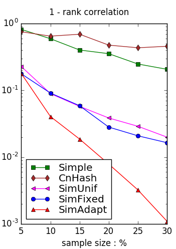
Figure 1: Dependence on bipartite edge sample rate fm\mathchar 29030_{\mathchar 29037}. Left: wre on Movie. Right: 1−C​o​r⁡(k)\mathchar 28721\mathchar 8704\mathop{\mathrm{\mathchar 28995\mathchar 29039\mathchar 29042}}\delimiter 67273472\mathchar 29035\delimiter 84054785 on GitHub. Top-100 dense ranks.

Accuracy and Bipartite Edge Sample Rate fm\mathchar 29030_{\mathchar 29037}. Figure 1 shows metric dependence on edge sample rate fm\mathchar 29030_{\mathchar 29037} for top-100 dense ranks, using wre on Movie (right) and 1−C​o​r\mathchar 28721\mathchar 8704\mathop{\mathrm{\mathchar 28995\mathchar 29039\mathchar 29042}} on GitHub (left). Each figure has curves for SimAdapt, SimFixed and SimUnif (and baseline methods CnHash and simple discussed below). We observe that SimAdapt obtains up to an order of magnitude reduction in both metrics for fm≥2​0%\mathchar 29030_{\mathchar 29037}\mathchar 12821\mathchar 28722\mathchar 28720\%.

Refer to caption Refer to caption
Figure 2: Dependence on rank. Left: wre on Movie. Right: 1−C​o​r⁡(k)\mathchar 28721\mathchar 8704\mathop{\mathrm{\mathchar 28995\mathchar 29039\mathchar 29042}}\delimiter 67273472\mathchar 29035\delimiter 84054785 on GitHub. Top-k\mathchar 29035 dense ranks for k\mathchar 29035 up to top-Max.

Accuracy and Similarity Rank. Figure 2 displays the same metric/data combinations as Figure 1 with fm=1​0%\mathchar 29030_{\mathchar 29037}\mathchar 12349\mathchar 28721\mathchar 28720\% for top-k\mathchar 29035 ranks as a function of k\mathchar 29035. As expected, SimAdapt is most accurate for lower ranks that it is designed to sample well, with wre 0.0​0​2\mathchar 28720\mathchar 314\mathchar 28720\mathchar 28720\mathchar 28722 for Movie at k=5​0\mathchar 29035\mathchar 12349\mathchar 28725\mathchar 28720 growing to about 0.2\mathchar 28720\mathchar 314\mathchar 28722 at maximum rank considered. SimUnif performed slightly better at high ranks, we believe because it was directing relatively more resources to high rank edges.

Accuracy and Aggregation Sampling Rate fn\mathchar 29030_{\mathchar 29038}. In all datasets the PBA second stage had little effect on accuracy for sampling rates fn\mathchar 29030_{\mathchar 29038} down to about 10% or less under a wide variety of parameter settings. Figure 3 shows results for SimFixed applied to Movie at fraction fm=1​0%\mathchar 29030_{\mathchar 29037}\mathchar 12349\mathchar 28721\mathchar 28720\% and PBA sampling rates of 5% and 15%, specifically wre and 1−C​o​r\mathchar 28721\mathchar 8704\mathop{\mathrm{\mathchar 28995\mathchar 29039\mathchar 29042}} for the top-k\mathchar 29035 dense ranks, as a function of k\mathchar 29035. For k\mathchar 29035 up to several hundred, even 5% PBA sampling has little or no effect, while errors roughly double when nearly all ranks are included. SimUnif, and to a lesser extent SimFixed, exhibited more noise, even at higher bipartite sampling rates fm\mathchar 29030_{\mathchar 29037}, which we attribute to a greater key diversity of updates (being less concentrated on high similarities) competing for space. Indeed, this noise was absent with exact aggregation.

Refer to caption
Figure 3: Sample based aggregation w/ PBA fn=5%,1​5%\mathchar 29030_{\mathchar 29038}\mathchar 12349\mathchar 28725\%\mathchar 24891\mathchar 28721\mathchar 28725\%, and none. Left: wre. Right: 1−C​o​r\mathchar 28721\mathchar 8704\mathop{\mathrm{\mathchar 28995\mathchar 29039\mathchar 29042}}, as function of top-k\mathchar 29035 ranks. Dataset Movie with SimFixed fm=1​0%\mathchar 29030_{\mathchar 29037}\mathchar 12349\mathchar 28721\mathchar 28720\% bipartite edge sampling.

Baseline Comparisons. Figures 1 and  2 include metric curves for the baseline methods simple and CnHash. SimAdapt and SimFixed typically performed better than simple by at least an order of magnitude. In some experiment with higher edge sample rate fm\mathchar 29030_{\mathchar 29037}, SimUnif was less accurate than simple, we believe due to the noise described above; Our methods performed noticeably better than CnHash in all cases, while CnHash was often no better than simple. The reasons for this are two-fold. First, in the streaming context, CnHash does not make maximal use of its constant space per vertex for nodes whose degree is less than maximum L\mathchar 29004. However, even counting only the stored edges, CnHash performs worse than our methods for storage use equivalent to our edge sampling rate fm<1​5%\mathchar 29030_{\mathchar 29037}\mathchar 12604\mathchar 28721\mathchar 28725\%. This second reason is the interaction of reservoir design with graph properties. Using shared edge buffer, SimAdapt and SimFixed devote resources to high adjacency edges associated with high similarity in a sparse graph. Edges incident at high degree nodes are more likely to acquire future adjacencies.

Noise reduction was employed for similarity estimates comprising a small number of updates. These exhibit noise from inverse probability estimators without the benefit of smoothing. We maintained an update count per edge and filtered estimates with count below a threshold. Most benefit was obtained by filtering estimates of update count below 10; this was used in all experiments reported above. Figure 4 compares the effects of no filtering (top) with filtering at threshold 10 (right) applied to SimAdapt with fm=\mathchar 29030_{\mathchar 29037}\mathchar 12349 10% edge sample, for the approximately 1,000 similarity edges in the top 100 estimated dense ranks. The left column shows actual and forecast weights. Without filtering, noise in the estimated similarity curve is due to a few edges whose estimated similarity greatly exceeds the actual similarity due to estimation noise, These are largely absent after filtering. The right column shows a scatter of (actual, forecast) ranks. Observe the cluster of edges with high actual rank (i.e. lower actual weight) and overestimated weight present with no filtering, that are removed by filtering.

Refer to caption Refer to caption
Figure 4: Noise and Filtering. GitHub fm=1​0%\mathchar 29030_{\mathchar 29037}\mathchar 12349\mathchar 28721\mathchar 28720\%. Top-100 dense ranked edges. Top: No filtering. Bottom: filter threshold 10. Left: forecast and actual weights. Right: scatter of (forecast, actual) ranks.

5 Related Work

A number of problems specific to bipartite graphs have recently attracted attention in the streaming or semi-streaming context. The classic problem of bipartite matching has been considered for semi-streaming Eggert et al. (2012); Kliemann (2011) and streaming Goel et al. (2012) data. Identifying top-k queries in graphs streams has been studied in Pan and Zhu (2012). The Adaptive Graph Priority Sampling of this paper builds on the graph priority sampling framework GPS in Ahmed et al. (2017) while the second sample aggregation method appears in Duffield et al. (2017). Graph stream sampling for subgraph counting is addressed in Ahmed et al. (2017); Jha et al. (2015); Stefani et al. (2017); Zakrzewska and Bader (2017); Ahmed et al. (2014a) amongst others; see Ahmed et al. (2014b) for a review. Zhao et al. (2016) is closer to our present work in that it provides a sample-based estimate of the CN count, albeit not specialized to the bipartite context. We make a detailed comparison of design and performance of Zhao et al. (2016) with our proposed approach in in Section 4.

6 Summary and Conclusion

This paper has proposed a sample-based estimator of the similarity (or projection graph) induced by a bipartite edge stream, i.e., the weighted graph whose edge weights or similarities are the numbers of common neighbors of its endpoint nodes. The statistical properties of real-world bipartite graphs provide an opportunity for weighted sampling that devotes resources to nodes with high similarity edges in the projected graph. Our proposed algorithm provides unbiased estimates of similarity graph edges in fixed storage without prior knowledge of the graph edge stream. With a relatively small sample of bipartite and the similarity graph edges (10% in each case), and with the enhancement of count based filtering of similarity edges at threshold 10, the sampled similarity edge set reproduces the actual similarities of sampled edges with errors of about 1​0−2\mathchar 28721\mathchar 28720^{\mathchar 8704\mathchar 28722} for top-100 dense estimate ranked edges, rising to an error of about 1​0−1\mathchar 28721\mathchar 28720^{\mathchar 8704\mathchar 28721} when most estimated edges are considered. Indeed, for the parameters used, the rank distribution of the sampled similarity graph is very similar to that of the actual graph for all but the highest ranks.

References

  • Ahmed et al. [2014a] N. K. Ahmed, N. Duffield, J. Neville, and R. Kompella. Graph sample and hold: A framework for big-graph analytics. In SIGKDD, 2014.
  • Ahmed et al. [2014b] N. K. Ahmed, J. Neville, and R. Kompella. Network sampling: From static to streaming graphs. In TKDD, 8(2):1–56, 2014.
  • Ahmed et al. [2017] Nesreen K. Ahmed, Nick Duffield, Theodore L. Willke, and Ryan A. Rossi. On sampling from massive graph streams. Proc. VLDB, 10(11):1430–1441, August 2017.
  • Andoni et al. [2011] A. Andoni, R. Krauthgamer, and K. Onak. Streaming algorithms via precision sampling. In 2011 IEEE 52nd Annual Symposium on Foundations of Computer Science, pages 363–372, Oct 2011.
  • Cohen et al. [2011] Edith Cohen, Nick Duffield, Haim Kaplan, Carsten Lund, and Mikkel Thorup. Efficient stream sampling for variance-optimal estimation of subset sums. SIAM J. Comput., 40(5):1402–1431, September 2011.
  • Cormen et al. [2001] Thomas H. Cormen, Clifford Stein, Ronald L. Rivest, and Charles E. Leiserson. Introduction to Algorithms. 2nd edition, 2001.
  • Duffield et al. [2017] Nick G. Duffield, Yunhong Xu, Liangzhen Xia, Nesreen K. Ahmed, and Minlan Yu. Stream aggregation through order sampling. In CIKM, 2017.
  • Eggert et al. [2012] Sebastian Eggert, Lasse Kliemann, Peter Munstermann, and Anand Srivastav. Bipartite matching in the semi-streaming model. Algorithmica, 63:490–508, 2012.
  • Estan and Varghese [2002] C. Estan and G. Varghese. New directions in traffic measurement and accounting. In Proc. ACM SIGCOMM ’2002, Pittsburgh, PA, 2002.
  • Fouss et al. [2007] Francois Fouss, Alain Pirotte, Jean-Michel Renders, and Marco Saerens. Random-walk computation of similarities between nodes of a graph with application to collaborative recommendation. IEEE Transactions on knowledge and data engineering, 19(3):355–369, 2007.
  • Goel et al. [2012] Ashish Goel, Michael Kapralov, and Sanjeev Khanna. On the communication and streaming complexity of maximum bipartite matching. In Proc. SODA ’12, pages 468–485, Philadelphia, PA, USA, 2012.
  • Gunawardana and Shani [2009] Asela Gunawardana and Guy Shani. A survey of accuracy evaluation metrics of recommendation tasks. J. Mach. Learn. Res., 10, 2009.
  • Herlocker et al. [2004] Jonathan L Herlocker, Joseph A Konstan, Loren G Terveen, and John T Riedl. Evaluating collaborative filtering recommender systems. ACM Transactions on Information Systems (TOIS), 22(1):5–53, 2004.
  • Horvitz and Thompson [1952] D. G. Horvitz and D. J. Thompson. A generalization of sampling without replacement from a finite universe. J. of the American Stat. Assoc., 47(260):663–685, 1952.
  • Jha et al. [2015] Madhav Jha, C. Seshadhri, and Ali Pinar. A space-efficient streaming algorithm for estimating transitivity and triangle counts using the birthday paradox. ACM Trans. Knowl. Discov. Data, 9(3):15:1–15:21, 2015.
  • Kliemann [2011] Lasse Kliemann. Matching in Bipartite Graph Streams in a Small Number of Passes, pages 254–266. Springer, Berlin, Heidelberg, 2011.
  • Koren [2008] Yehuda Koren. Factorization meets the neighborhood: a multifaceted collaborative filtering model. In Proceedings of the 14th ACM SIGKDD international conference on Knowledge discovery and data mining, pages 426–434. ACM, 2008.
  • Liben-Nowell and Kleinberg [2007] David Liben-Nowell and Jon Kleinberg. The link-prediction problem for social networks. journal of the Association for Information Science and Technology, 58(7):1019–1031, 2007.
  • Monemizadeh and Woodruff [2010] M. Monemizadeh and D. P. Woodruff. 1-pass relative-error lp{}_{\mbox{p}}-sampling with applications. In Proc. 21st ACM-SIAM Symposium on Discrete Algorithms. ACM-SIAM, 2010.
  • Muthukrishnan [2005] S. Muthukrishnan. Data streams: Algorithms and applications. Now Publishers Inc, 2005.
  • Ning et al. [2015] Xia Ning, Christian Desrosiers, and George Karypis. A Comprehensive Survey of Neighborhood-Based Recommendation Methods, pages 37–76. Springer US, Boston, MA, 2015.
  • Pan and Zhu [2012] Shirui Pan and Xingquan Zhu. Continuous top-k query for graph streams. In Proc. CIKM ’12, pages 2659–2662, New York, NY, USA, 2012.
  • Rossi and Ahmed [2015] Ryan A. Rossi and Nesreen K. Ahmed. The network data repository with interactive graph analytics and visualization. In AAAI, 2015. http://networkrepository.com.
  • Salton et al. [1993] Gerard Salton, James Allan, and Chris Buckley. Approaches to passage retrieval in full text information systems. In ACM SIGIR 1993, pages 49–58. ACM, 1993.
  • Stefani et al. [2017] Lorenzo De Stefani, Alessandro Epasto, Matteo Riondato, and Eli Upfal. TriÈst: Counting local and global triangles in fully dynamic streams with fixed memory size. ACM TKDD, 11(4):43:1–43:50, 2017.
  • Tillé [2006] Y. Tillé. Sampling Algorithms. Springer-Verlag, 2006.
  • Zakrzewska and Bader [2017] Anita Zakrzewska and David A Bader. Streaming graph sampling with size restrictions. In IEEE/ACM International Conference on Advances in Social Networks Analysis and Mining, 2017.
  • Zhao et al. [2016] P. Zhao, C. Aggarwal, and G. He. Link prediction in graph streams. In Proc. ICDE ’16, pages 553–564, May 2016.
  • Zhou et al. [2007] Tao Zhou, Jie Ren, Matúš Medo, and Yi-Cheng Zhang. Bipartite network projection and personal recommendation. Physical Review E, 76(4):046115, 2007.