Rank Pruning for Dominance Queries in CP-Nets

Definition 1: Conditional Preference Network (CP-Net) (Boutilier et al., 2004a, ). A CP-net $N$, over variables $V$, is a directed graph $G$, with nodes $V$. Each node $X$, is annotated with a conditional preference table CPT$(X)$. For any $X\in V$, $\text{CPT}(X)$ gives, for each possible assignment of values to Pa$(X)$ (the parent variables of $X$ in $G$), the user’s order of ceteris paribus preference over all possible values $X$ can take (that is, the domain of $X$, Dom$(X)$). We assume all variables to have discrete domains.

The graph $G$ is a preferential dependency graph with the following underlying assumption. For any $X,Y\in V$, $X$ is preferentially independent of $Y$ given Pa$(X)$. That is, once Pa$(X)$ have been assigned values, the user’s preference over Dom$(X)$ is fixed and not affected by the value taken by $Y$. To illustrate these ideas, consider the following example.

Example 1. Suppose again that we are modelling a user’s preference over aeroplane seats. The variables we might take into account, and their respective domains, are as follows.

$A=\text{Flight Length }\hskip 14.22636pt$	$\text{Dom}(A)=\{a:\text{short, }\bar{a}:\text{long-haul}\}$
$B=\text{School Term Time }\hskip 14.22636pt$	$\text{Dom}(B)=\{b:\text{term, }\bar{b}:\text{holiday}\}$
$C=\text{Class }\hskip 14.22636pt$	$\text{Dom}(C)=\{c:\text{economy, }\bar{c}:\text{business, }\bar{\bar{c}}:\text{first}\}$
$D=\text{Pay Extra for Wi-Fi }\hskip 14.22636pt$	$\text{Dom}(D)=\{d:\text{no, }\bar{d}:\text{yes}\}$

One example of a CP-net over these variables is given in Figure 1. The structure of this CP-net shows that the user has a strict preference for short flights over long-haul flights (ceteris paribus, that is, given $B,C,D$ take the same values) and for flying in term time over flying in holiday time (ceteris paribus, that is, given $A,C,D$ take the same values). These preferences are unaffected by the values taken by any other variable. However, the user’s preference for which class they fly in is dependent (conditional) upon the values taken by $A$ and $B$ (Flight Length and School Term Time). If it is a short flight in term time, then the user prefers economy to business to first class (ceteris paribus- given that $D$ takes the same value). However, if it is a short flight in holiday time, then the user prefers business to first to economy class. Once the values of $A$ and $B$ are determined, these preferences over $C$ (Class) are fixed and do not change (regardless of the value taken by $D$), by our preferential independence assumption above. Similarly, the user’s preference over $D$ (Pay Extra for Wi-Fi) depends on the value taken by $C$, but these preferences are independent of the values taken by $A$ and $B$.

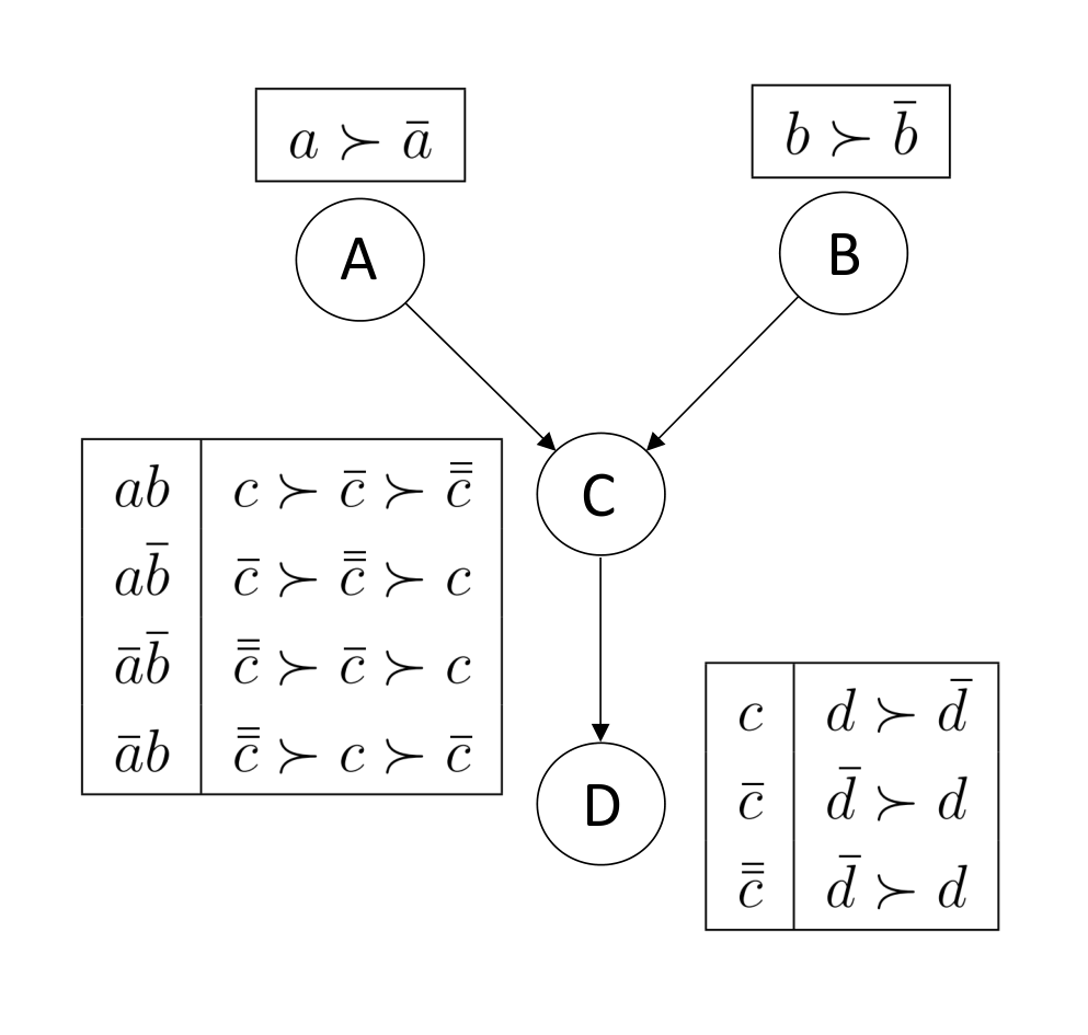
We assume throughout this paper that we are dealing with CP-nets whose directed graph (structure) is acyclic. When we refer to binary CP-nets we mean CP-nets where all variables are binary. For the majority of this paper (except §7), we assume that every row of the conditional preference tables (CPTs) contains a strict complete order of the appropriate domain. In §7, we discuss how our results can be generalised to apply to cases where the CPTs may express indifference between values. This is an important extension because indifference is a natural notion that we may reasonably expect people to express when specifying their preferences.

Given a CP-net $N$, over variables $V=\{V_{1},V_{2},...,V_{n}\}$, an outcome $o$, is an $n$-tuple representing an assignment of values to all variables, $o\in$ Dom$(V_{1})\times$ Dom$(V_{2})\times\cdots\times$ Dom$(V_{n})$. Let $\Omega$ denote the set of all outcomes, then $|\Omega|=|\text{Dom}(V_{1})|\times|\text{Dom}(V_{2})|\times\cdots\times|\text{Dom}(V_{n})|$. For our previous example, $a\bar{b}\bar{\bar{c}}\bar{d}$ is an example of an outcome (specifically this is a short flight in holiday time, sitting in first class with Wi-Fi). In total, there are 24 possible outcomes for the CP-net given in Example 1. In general, $|\Omega|\geq 2^{n}$ with equality only in the case of binary CP-nets.

The preference graph associated with $N$ is a directed graph $G_{N}$, with the outcomes $\Omega$ as nodes and edges defined as follows. Let $o,o^{\prime}\in\Omega$, then there is an edge $o\rightarrow o^{\prime}$ if and only if $o$ and $o^{\prime}$ differ on the value assigned to exactly one variable, say $X$, and, in the row of $\text{CPT}(X)$ corresponding to the assignment of values to Pa$(X)$ in both $o$ and $o^{\prime}$, the value of $X$ taken in $o^{\prime}$ is preferred to that in $o$. As the preference statements in the CPTs of a CP-net are all ceteris paribus, they only encode preferences between outcome pairs that differ on exactly one variable. Thus, the edges in the preference graph (and their transitive closure) represent all known preference information about the user. That is, it is an equivalent representation to the CP-net itself. (Boutilier et al., 2004a, )

Definition 2: Entailment. Let $N$ be a CP-net with associated preference graph $G_{N}$, and two associated outcomes $o$ and $o^{\prime}$. We say that $N$ entails the relation ‘$o$ is preferred to $o^{\prime}$’, denoted $N\vDash o\succ o^{\prime}$, if and only if there is a directed path $o^{\prime}\leadsto o$ in $G_{N}$.

The entailed relations are all of the user preferences between outcome pairs encoded in the CP-net. A consistent ordering for a CP-net is a complete ordering of the outcomes $\Omega$, that obeys all known (entailed) preference information about the user. Equivalently, a consistent ordering is any ordering of $\Omega$ such that if there is a path $o\leadsto o^{\prime}$ in the preference graph, then $o^{\prime}$ comes before $o$ in the ordering (that is, any topological ordering of the preference graph). Notice that entailed relations hold in all consistent orderings. Further, as we are considering only acyclic CP-nets, there will always be at least one consistent ordering (Boutilier et al., 2004a, ).

Remark 1. The above definitions for entailment and consistent orderings are equivalent but not identical to those given by Boutilier et al., 2004a (). Boutilier et al., 2004a () define orderings that satisfy the CP-net (consistent orderings) to be complete orderings of the outcomes that obey all of the ceteris paribus preference statements given in the CPTs. They go on to define entailment as $N\vDash o\succ o^{\prime}$ if and only if $o$ comes before $o^{\prime}$ in all consistent orderings. Boutilier et al., 2004a () show their definition of entailment to be equivalent to the above definition. For consistent orderings, it is clear that the two definitions are equivalent as the preference graph is an equivalent representation of the CP-net. Thus, an ordering that respects the CPTs is equivalent to an ordering that respects the preference graph. We use the above definitions for simplicity. As we are using equivalent definitions, all results by Boutilier et al., 2004a () continue to hold.

Definition 3: Dominance Query (Boutilier et al., 2004a, ). Let $N$ be a CP-net, and let $o$ and $o^{\prime}$ be associated outcomes. A dominance query asks whether $N\vDash o\succ o^{\prime}$ holds.

This dominance query holds if and only if there is a directed path $o^{\prime}\leadsto o$ in the associated preference graph. That is, there is a sequence of outcomes $o^{\prime}=o_{1},o_{2},...,o_{m}=o$ such that $o_{i}$ and $o_{i+1}$ differ on the value of exactly one variable and $N\vDash o_{i+1}\succ o_{i}$. We call this type of outcome sequence an improving flipping sequence (IFS). Thus, dominance queries can be reframed as a search for an IFS between the outcomes of interest; this is how we approach dominance queries later on in this paper. (Boutilier et al., 2004a, )

Finally, a short remark on notation. Let $N$ be a CP-net over variables $V$, and let $o$ be an associated outcome. Let $X\in V$ and $Y\subseteq V$. For ease of notation, let $o[X]$ denote the value assigned to $X$ in $o$ and let $o[Y]$ be the $|Y|$-tuple of values assigned to $Y$ in $o$. Further, if $Y=\{Y_{1},Y_{2},...,Y_{k}\}$ then let $\text{Dom}(Y)$ denote $\text{Dom}(Y_{1})\times\text{Dom}(Y_{2})\times\cdots\times\text{Dom}(Y_{k})$. That is, $\text{Dom}(Y)$ consists of all $|Y|$-tuples of values that may be assigned to $Y$.

Let $N$ be a CP-net over variables $V$. We have mentioned previously that the associated preference graph is an equivalent representation of this information. Another equivalent way of representing CP-nets is by an event tree (Edwards,, 1983). We use this alternate representation to motivate and construct our quantification of user preference in §3.1. The event tree representation of $N$, denoted $T(N)$, can be constructed in three steps.

First, put the variables in a topological order according to the CP-net structure,$V=\{V_{1},...,V_{n}\}$. That is, Pa$(V_{i})\subseteq\{V_{1},...,V_{i-1}\}$. For the CP-net given in Example 1, there are two such orderings, $ABCD$ and $BACD$. We use $ABCD$ for simplicity.

Second, construct an event tree representing the successive events of $V_{1}$ taking a value, then $V_{2}$ taking a value, and so on up to $V_{n}$. The root node branches into $|\text{Dom}(V_{1})|$ possibilities (each branch should be labelled with an associated element of $\text{Dom}(V_{1})$). Then, each of these nodes branches into $|\text{Dom}(V_{2})|$ possibilities (each labelled with an associated element of $\text{Dom}(V_{2})$). And so on until each of $V_{1},V_{2},...,V_{n}$ have taken a value. The final tree has $|\Omega|$ root-to-leaf paths, corresponding to the outcomes. Figure 2 gives the event tree representation for the CP-net in Example 1 (ignore the branch weights for the moment).

Finally, the branches need to be labelled with the level of preference of the associated variable assignment. Suppose we are labelling the branch $b$, which represents that $X=x$ (for some $X\in V$). By inspecting the unique path from the root to the start of $b$, identify the values assigned to Pa$(X)$. From the appropriate row of $\text{CPT}(X)$, you can identify the position of preference of the choice $X=x$. If $x$ is the best choice under this assignment to Pa$(X)$, then label $b$ with ‘$1^{st}$’, if it is the second best, then label it ‘$2^{nd}$’, and so on. For our running example, at the first stage, we would label the $A=a$ branch ‘$1^{st}$’ and the $A=\bar{a}$ branch ‘$2^{nd}$’ because of $\text{CPT}(A)$. Similarly, both $B=b$ branches have the label ‘$1^{st}$’ and both $B=\bar{b}$ branches have the label ‘$2^{nd}$’. Now, consider the top-most instance of the tree branching into the options for $C$ ($c,\bar{c},\bar{\bar{c}}$). At this point $A$ and $B$ have been assigned values $a$ and $b$ and so we are concerned with this (top) row of $\text{CPT}(C)$. From the CPT, we can see that, given the history of this path, $c$ is preferred to $\bar{c}$ is preferred to $\bar{\bar{c}}$, thus we give the $C=c$ branch the label ‘$1^{st}$’, the $C=\bar{c}$ branch the label ‘$2^{nd}$’, and the $C=\bar{\bar{c}}$ branch the label ‘$3^{rd}$’. Labelling the rest of the $C$ and $D$ branches is a similar process. However, for the $D$ branches we only need to look at the value previously taken by $C$ to determine which $\text{CPT}(D)$ row to consult.

From the example used above, it is clear that $T(N)$ can become very large even for smaller CP-nets. As mentioned previously, we use this event tree representation to aid the construction of our outcome ranks in §3.1. However, in §4 we demonstrate that constructing this tree is not necessary for their calculation, so the exponential size of the trees is not a limitation.

Remark 2. This event tree representation, $T(N)$, is equivalent to the original CP-net (recalling that the CP-net consists of both the structure and the CPTs). Clearly, one can construct $T(N)$ from $N$; this process is described above. The key part to this claim is that one can reconstruct $N$ given $T(N)$. A sketch of this process is as follows. From $T(N)$ we can read off the domains of the variables and a topological ordering. Suppose $X_{1},X_{2},...,X_{n}$ is this topological ordering, then $\text{Pa}(X_{i})\subseteq\{X_{1},...,X_{i-1}\}$. If $Y\in\{X_{1},...,X_{i-1}\}$, then $Y\in\text{Pa}(X_{i})$ if and only if there are two direct paths $p$ and $p^{\prime}$, of length $(i-1)$ that begin at the root of $T(N)$ and have the following property. By definition, $p$ and $p^{\prime}$ assign values to $\{X_{1},...,X_{i-1}\}$ only. We must have that $p$ and $p^{\prime}$ differ only on the value assigned to $Y$ and that the preference order over $X_{i}$ is different for these two assignments. That is, the labelling of the branches corresponding to the different values of $X_{i}$ that come directly after path $p$ is different to those after $p^{\prime}$. Identifying the parent sets determines the structure of $N$ and it only remains to construct the CPTs. Given the parents of a variable and their respective domains, we know already the set of all parent assignments that corresponds to the rows of the CPTs. Given a row of $\text{CPT}(X_{i})$, that is, an assignment of values to $\text{Pa}(X_{i})$, say $u_{i}$, we need to recover the corresponding preference order over $X_{i}$. This can be done by finding any path $p$ of length $(i-1)$ that begins at the root of $T(N)$ and assigns $\text{Pa}(X_{i})$ the values in $u_{i}$. The relevant preference order over $X_{i}$ can be read off from the labels on the branches corresponding to the different values of $X_{i}$ that come directly after $p$; the value of $X_{i}$ assigned the label ‘$1^{st}$’ is first in the preference order (most preferred), the value assigned the label ‘$2^{nd}$’ is second and so on. We have now completely constructed the CPTs and, thus, $N$.

In this section, we introduce our outcome ranks (which successfully induce a consistent ordering of the outcomes). These are obtained using the event tree representation discussed in §2.2. Specifically, we first weight the edges of the event tree representation and then read off the rank of an outcome from this weighted tree. The ranking we construct reflects user preference so more preferred outcomes have higher scores.

To motivate our weighting convention for the edges of $T(N)$, we must look at what determines the user’s level of preference for an outcome $o$. The position of preference of the values taken by the individual variables, according to the CPTs, needs to be taken into account. However, according to the semantics of CP-nets, ancestor variables in the CP-net structure are more important to the user than their descendants (Boutilier et al., 2004a, ). Thus, if variable $A$ is an ancestor of variable $B$, then when quantifying user preference over outcomes, we must have a larger penalty for a decrease of preference for $A$ than for a decrease of preference for $B$. Therefore, the position of variables in the CP-net structure will need to be taken into account in determining the user’s level of preference for an outcome.

As we are allowing our CP-net variables to be multivalued, we must also take into account how domain size affects user preference. By the semantics of CP-nets, domain size should be independent of the importance of a variable. Suppose we have variables $X$ and $Y$ such that $Y$ is a descendant of $X$ in the CP-net. Then any decrease of preference in $X$ should dominate any decrease of preference in $Y$, regardless of their domain sizes. Thus, our quantification of preference must also have this property.

Motivated by these restrictions imposed by the CP-net semantics, we have created the following weighting for the branches of the event tree representation of a CP-net. Let $N$ be a CP-net over variables $V=\{X_{1},..,X_{n}\}$ and assume that this ordering of the variables is a topological ordering with respect to the structure of $N$. Now, consider the event tree representation of $N$, $T(N)$. Let $e$ be the edge of $T(N)$ that indicates variable $X_{i}$ takes value $x_{i}$ given $X_{1},...,X_{i-1}$ take values $x_{1},...,x_{i-1}$. Use $p$ to denote the directed path from the root of $T(N)$ to the start of $e$, that dictates in turn that $X_{1}=x_{1}$, $X_{2}=x_{2},...,X_{i-1}=x_{i-1}$. Let $u_{i}\in\text{Dom}(\text{Pa}(X_{i}))$ be the assignment of values to the parents of $X_{i}$ dictated by $p$. We attach the following weight to $e$:

$$\Bigg(\prod_{Y\in\text{Anc}(X_{i})}\frac{1}{n_{Y}}\Bigg)(d_{X_{i}}+1)\frac{n_{X_{i}}-k+1}{n_{X_{i}}},$$

(1)

which uses the following notation:

• $\textendash$

  $\text{Anc}(X_{i})$ is the set of variables $Y\in V$ such that there is a directed path $Y\leadsto X_{i}$ in the structure of $N$ (these are referred to as the ancestors of $X_{i}$),

• $\textendash$

  $n_{X_{i}}:=|\text{Dom}(X_{i})|$,

• $\textendash$

  $d_{X_{i}}$ is the number of distinct directed paths of any length in the structure of $N$ that originate at ${X_{i}}$ (the number of descendent paths of $X_{i}$),

• $\textendash$

  $k$ is the position of preference of the choice of $X_{i}=x_{i}$ given Pa$(X_{i})=u_{i}$. So, if $X_{i}=x_{i}$ is the best choice for the user, then $k=1$, if it is the second best choice, then $k=2$, and so on. If it is the worst possible choice for $X_{i}$, then $k=|\text{Dom}(X_{i})|$.

We refer to the leftmost product term in (1) as the ancestral factor of $X_{i}$, $AF_{X_{i}}$. This factor scales the weight down by the size of $X_{i}$’s ancestors’ domains. The purpose of this is so that any decrease in preference of an ancestor will dominate a decrease in preference of $X_{i}$, regardless of the size of the ancestor’s domain relative to $|\text{Dom}(X_{i})|$.

Consider the central term of (1), $(d_{X_{i}}+1)$. If $X$ is an ancestor of $Y$, then $d_{X}>d_{Y}$. An ancestor variable is more important to the user than its descendent variables, this term allocates these more important variables more weight. In particular, this term ensures that reductions in preference of an ancestor variable have larger penalties than reductions in preference of a descendant.

We refer to the rightmost product term in (1) as the preference position of the choice $X_{i}=x_{i}$ given Pa$(X_{i})=u_{i}$, denoted $P_{P}\{X_{i}=x_{i}\hskip 2.84544pt|\hskip 2.84544pt\text{Pa}(X_{i})=u_{i}\}$. This is a value in $\{1/n_{X_{i}},2/n_{X_{i}},...,(n_{X_{i}}-1)/n_{X_{i}},1\}$. This is simply a factor on the (0,1] scale indicating to what degree the user prefers this choice of value for $X_{i}$. This naturally impacts the user’s preference for the overall outcome. This factor gets larger for more preferred values with the best value assigned preference position 1.

Notice that the preference position factor decreases in equal increments. Due to a lack of information provided by the CP-net, we cannot justify a more complex increment when quantitatively representing the user’s preferences over $\text{Dom}(X_{i})$. Consider a variable $A$ with $\text{Dom}(A)=\{a_{1},a_{2},a_{3}\}$ and CPT $a_{1}\succ a_{2}\succ a_{3}$. This could mean that, to the user, $a_{2}$ is slightly worse than $a_{1}$, but $a_{3}$ is much worse than $a_{2}$. Alternatively, it could be that $a_{2}$ is much worse than $a_{1}$, but $a_{3}$ is only slightly worse than $a_{2}$. We cannot determine which of these is the case due to lack of information, and so we assume that preference decreases in equal increments each time. In this situation, our preference positions would be $1,\frac{2}{3}$, and $\frac{1}{3}$ for $a_{1},a_{2},$ and $a_{3}$ respectively.

We refer to the event tree representation of $N$ weighted using the above convention as the weighted tree representation of $N$, $W(N)$.

Example 2. We now return to the CP-net $N$, from Example 1 and corresponding event tree $T(N)$, given in §2.2. Simple examination of the CP-net structure and CPTs gives us the following information:

$$\text{Anc}(A)=\varnothing,\hskip 5.69046pt\text{Anc}(B)=\varnothing,\hskip 5.69046pt\text{Anc}(C)=\{A,B\},\hskip 5.69046pt\text{Anc}(D)=\{A,B,C\},$$

$$n_{A}=2,\hskip 5.69046ptn_{B}=2,\hskip 5.69046ptn_{C}=3,\hskip 5.69046ptn_{D}=2,$$

$$d_{A}=2,\hskip 5.69046ptd_{B}=2,\hskip 5.69046ptd_{C}=1,\hskip 5.69046ptd_{D}=0.$$

From the $n_{X}$ values and the ancestor sets, we can calculate the ancestral factor of each variable:

$$AF_{A}=1,\hskip 5.69046ptAF_{B}=1,$$

$$AF_{C}=\frac{1}{2}\times\frac{1}{2}=\frac{1}{4},$$

$$AF_{D}=\frac{1}{2}\times\frac{1}{2}\times\frac{1}{3}=\frac{1}{12}.$$

We can now use these values and the CPTs to directly calculate the edge weights and thus construct the weighted tree representation of this example. $W(N)$ is given in Figure 2 with the preference positions given in bold.

By examining the weighted tree for this example, it can be seen that the weights attached to any two edges indicating the value taken by the same variable differ only on the preference position (the bolded number). Consider the set of edges leaving any node in the tree. By the definition of preference position, those edges indicating that the next variable takes a more preferred value will have larger weights. Thus, we can recover $T(N)$ given $W(N)$. As $T(N)$ is an equivalent representation to $N$, this shows that $W(N)$ is also an equivalent representation to $N$. Recall that $N$ is both the CP-net structure and the CPTs.

For ease of notation we shall, from this point on, simplify the notation for the weighted tree representation of $N$ from $W(N)$ to $W$ without ambiguity.

Now that we can construct the weighted tree representation of any given CP-net, we use this structure to define our quantitative measure of preference for any outcome.

Definition 4: Rank. Given a CP-net $N$, and an associated outcome $o$, we define the rank of $o$, $r(o)$, to be the sum of the weights on the edges of the root-to-leaf path of $W$ that corresponds to $o$.

Example 3. Continuing on from Example 2, we calculate the ranks of several outcomes directly from $W$:

$$\begin{split}r(\bar{a}b\bar{\bar{c}}\bar{d})=&\bigg[1\cdot(2+1)\cdot\frac{1}{2}\bigg]+\bigg[1\cdot(2+1)\cdot 1\bigg]+\bigg[\frac{1}{4}\cdot(1+1)\cdot 1\bigg]+\bigg[\frac{1}{12}\cdot(0+1)\cdot 1\bigg]\\ =&\hskip 2.84544pt\frac{61}{12},\\ &\\ r(ab\bar{c}\bar{d})=&\bigg[1\cdot(2+1)\cdot 1\bigg]+\bigg[1\cdot(2+1)\cdot 1\bigg]+\bigg[\frac{1}{4}\cdot(1+1)\cdot\frac{2}{3}\bigg]+\bigg[\frac{1}{12}\cdot(0+1)\cdot 1\bigg]\\ =&\frac{77}{12},\\ &\\ r(\bar{a}\bar{b}cd)=&\bigg[1\cdot(2+1)\cdot\frac{1}{2}\bigg]+\bigg[1\cdot(2+1)\cdot\frac{1}{2}\bigg]+\bigg[\frac{1}{4}\cdot(1+1)\cdot\frac{1}{3}\bigg]+\bigg[\frac{1}{12}\cdot(0+1)\cdot 1\bigg]\\ =&\frac{39}{12}.\end{split}$$

Recall that our aim was to assign higher values to more preferred outcomes. Thus, the relative sizes of these ranks are as we would expect as we can derive the following sequences of preference directly from the CPTs:

$$ab\bar{c}\bar{d}\succ ab\bar{\bar{c}}\bar{d}\succ\bar{a}b\bar{\bar{c}}\bar{d}$$

$$\bar{a}b\bar{\bar{c}}\bar{d}\succ\bar{a}b\bar{\bar{c}}d\succ\bar{a}bcd\succ\bar{a}\bar{b}cd$$

Thus, we have $N\models ab\bar{c}\bar{d}\succ\bar{a}b\bar{\bar{c}}\bar{d}\succ\bar{a}\bar{b}cd$ and $r(ab\bar{c}\bar{d})>r(\bar{a}b\bar{\bar{c}}\bar{d})>r(\bar{a}\bar{b}cd)$.

In this section we demonstrate how our outcome ranks can be used to obtain consistent orderings. This can be applied to the whole outcome set, in order to get a complete consistent ordering for the CP-net, or to any subset of the outcomes. Further, this method can be directly applied to CP-nets with additional plausibility constraints.

There are several methods of obtaining a consistent ordering in the existing literature, some of which we outline below. As discussed in §1, Domshlak et al., (2003) use their approximations to obtain consistent orderings. The penalty function defined by Li et al., (2011) could also be used to obtain a consistent ordering in this manner, although this is not mentioned in their paper. The utility function defined by McGeachie and Doyle, (2002) would induce a consistent ordering, if the utility was based upon CP-net preferences. Sun et al., (2017) utilise their complete preference table in order to obtain consistent orderings. Boutilier et al., 2004a () take yet another approach which is to construct a lexicographic ordering of the outcomes as follows. Let $N$ be a CP-net with variables $\{X_{1},...,X_{n}\}$, listed such that a variable’s parents come before the variable itself. Suppose we have two outcomes $o_{1}$ and $o_{2}$, that have the same values for $X_{1},...,X_{k}$ but differ on the value of $X_{k+1}$, say $o_{1}[X_{k+1}]=x_{k+1}$ and $o_{2}[X_{k+1}]=x^{\prime}_{k+1}$. If, given the assignment of values to Pa$(X_{k+1})$ in both $o_{1}$ and $o_{2}$, $\text{CPT}(X_{k+1})$ dictates that $x_{k+1}\succ x^{\prime}_{k+1}$, then $o_{1}$ comes before $o_{2}$ in this ordering.

As we have constructed our outcome ranks to reflect user preference, they obey all entailed relations, as we wanted. Thus, our ranks induce a consistent ordering of the outcomes, $\succ^{*}$. This $\succ^{*}$ is obtained simply by ordering the outcomes according to their rank, with outcomes with higher ranks considered to be more preferred. Proof of these claims is given below.

Theorem 1. Given a CP-net $N$, for any outcomes $o$ and $o^{\prime}$, we have that $N\models o\succ o^{\prime}\Rightarrow r(o)>r(o^{\prime})$.

Proof given in Appendix A.

This tells us that if the CP-net dictates that the user prefers $o$ to $o^{\prime}$, then $r(o)>r(o^{\prime})$, that is, $o\succ^{*}o^{\prime}$. In fact, we can say more than $r(o)>r(o^{\prime})$; we can find a lower bound for the rank difference, $r(o)-r(o^{\prime})$. Details of this lower bound are given in §5.

Corollary 1. Given a CP-net $N$, and two distinct associated outcomes $o$ and $o^{\prime}$, $r(o)=r(o^{\prime})\Rightarrow N\nvDash o\succ o^{\prime}\wedge N\nvDash o^{\prime}\succ o$ (we say that $o$ and $o^{\prime}$ are incomparable).

Corollary 2. Let $N$ be a CP-net. Let $\succ^{*}$ be the ordering of the outcomes of $N$ induced by the outcome ranks. Then $\succ^{*}$ is a consistent ordering of the outcomes with respect to $N$.

We cannot guarantee $\succ^{*}$ is a strict order. There is a possibility that two distinct outcomes $o$ and $o^{\prime}$ could be assigned equal rank. However, Corollary 1 shows that this can only occur when we do not know which the user prefers. If we want a strict ordering of the outcomes, then it is enough to force any outcomes with equal ranks into an arbitrary order. Any strict ordering of the outcomes obtained from $\succ^{*}$ in this manner is a consistent ordering of the outcomes as we have only altered the order of incomparable outcomes.

We have now introduced a novel method of quantifying user preference and obtaining a consistent outcome ordering given any (possibly multivalued) acyclic CP-net. Further, we can ensure that this is a strict ordering of the outcomes. From now on, when we refer to the outcome ordering induced by outcome ranks, we are referring to a strict ordering.

Remark 3. Going from a CP-net to a consistent ordering gives the impression of losing a great deal of information, especially as there are likely to be many consistent orderings and we have constructed one that is no better than any other. Moreover, the process of forcing our ordering to be strict arbitrarily discards several possible orderings. However, we have found that, given this consistent ordering, we can answer ordering and dominance queries directly, without needing to consult the CP-net. Further, we can use these ranks to improve the efficiency of answering dominance queries. We can also determine whether $o\succ^{*}o^{\prime}$ is entailed by the CP-net ($N\models o\succ o^{\prime}$) or constructed ($N\nvDash o\succ o^{\prime}\wedge N\nvDash o^{\prime}\succ o$), and update $\succ^{*}$ given new (consistent) preference information, both without consulting the CP-net. In fact, despite constructing a consistent ordering somewhat arbitrarily, we have not lost any information at all. In this paper, we focus on demonstrating how these ranks can be used to improve the efficiency of answering dominance queries. The other results discussed above are explored in a forthcoming paper.

Example 4 For the CP-net in Example 1, the ordering of the outcomes induced by the ranks is as follows:

$$\begin{split}abcd\succ^{*}abc\bar{d}\succ^{*}ab\bar{c}\bar{d}\succ^{*}ab\bar{c}d&\succ^{*}ab\bar{\bar{c}}\bar{d}\succ^{*}ab\bar{\bar{c}}d\succ^{*}a\bar{b}\bar{c}\bar{d}=\bar{a}b\bar{\bar{c}}\bar{d}\succ^{*}\\ a\bar{b}\bar{c}d=\bar{a}b\bar{\bar{c}}d\succ^{*}a\bar{b}\bar{\bar{c}}\bar{d}=\bar{a}bcd&\succ^{*}a\bar{b}\bar{\bar{c}}d=\bar{a}bc\bar{d}\succ^{*}a\bar{b}cd=\bar{a}b\bar{c}\bar{d}\succ^{*}\\ a\bar{b}c\bar{d}=\bar{a}b\bar{c}d\succ^{*}\bar{a}\bar{b}\bar{\bar{c}}\bar{d}\succ^{*}\bar{a}\bar{b}\bar{\bar{c}}d&\succ^{*}\bar{a}\bar{b}\bar{c}\bar{d}\succ^{*}\bar{a}\bar{b}\bar{c}d\succ^{*}\bar{a}\bar{b}cd\succ^{*}\bar{a}\bar{b}c\bar{d}.\\ \end{split}$$

We can obtain a strict ordering of the outcomes simply by replacing each $=$ with a $\succ^{*}$.

Our method of obtaining a consistent ordering using outcome ranks has the advantage of how easily it can be adapted to find a consistent ordering of any subset of the outcomes. Let $N$ be a CP-net over variables $V$ and let $O$ be some subset of the outcomes, $O\subseteq\Omega$. Suppose we wish to put these outcomes $O$, in an order that agrees with everything the CP-net tells us about the user’s preference. That is, we wish to find a strict order over $O$, $\succ_{O}$, such that for any two outcomes $o_{1},o_{2}\in O$, we have that $N\vDash o_{1}\succ o_{2}\implies o_{1}\succ_{O}o_{2}$. To motivate the consistent ordering of subsets, consider an online shopping website displaying its products and suppose the seller wishes to promote a certain range of items; the seller would want exactly these items to appear on the first page. Putting these selected items into an order such that those items of more interest to the client are higher up, is an example of why we might want to put a specified subset of outcomes into a consistent order.

A consistent ordering of $O\subseteq\Omega$ can be obtained in exactly the same way we obtained a consistent ordering for $N$. For each $o\in O$, calculate the rank of $o$, $r(o)$, and then order $O$ according to rank value. To get a strict consistent ordering of $O$, force outcomes of equal rank into an arbitrary order. Call this strict ordering of $O$ $\succ_{O}$. We can see that $\succ_{O}$ is a consistent ordering of $O$ by using exactly the same reasoning we used to show that $\succ^{*}$ is a consistent ordering. Another way to obtain $\succ_{O}$ is to construct $\succ^{*}$ and then restrict the ordering to $O$ but this is less efficient.

In §4, we present an algorithm that can calculate $r(o)$ for any outcome in time $O(|V|^{4})$. Thus, a consistent ordering for a subset of size $k$ can be obtained as described above in $O(|V|^{4}k+k^{2})$ time. Boutilier et al., 2004a () also proposed a solution to the problem of obtaining a consistent ordering for any subset of the outcomes. They proposed finding a consistent ordering of $O$ by repeatedly answering ordering queries (an ordering query essentially asks, given two outcomes, find a consistent ordering of the two). Using this method, a consistent ordering for a subset of size $k$ can be obtained in $O(|V|k^{2})$ time (as their method of answering ordering queries has complexity $O(|V|)$). Thus, for larger subsets of the outcomes, our method becomes more efficient. This is because every ordering query has complexity $O(|V|)$, whereas, in our method, once the ranks are calculated the problem is reduced to a simple sorting task. Note that the number of outcomes is at least $2^{|V|}$ (with equality only in the case of binary CP-nets), so subsets of the outcomes can get very large even for relatively small CP-nets.

A particularly interesting application of being able to consistently order any subset of the outcomes is finding a consistent ordering for CP-nets that have additional plausibility constraints. That is, a CP-net such that a specified proper subset of the outcomes, say $P\subsetneq\Omega$, are possible and the remainder are considered impossible. In reality, this kind of asymmetry in a CP-net system is commonplace. Consider, for example, an airline where there are no flights between specified dates and destinations with available business class seats, this would then be an impossible outcome.

Lemma 1. Given a CP-net $N$, and the further constraint that the only outcomes that are possible are those contained in $P\subset\Omega$, call the CP-net with these added constraints $N_{C}$. Let $\succ_{P}$ be any strict ordering over $P$ such that, for all $o,o^{\prime}\in P$, we have $N\vDash o\succ o^{\prime}\implies o\succ_{P}o^{\prime}$. Then $\succ_{P}$ is a consistent ordering for $N_{C}$.

By Lemma 1, every consistent ordering (with respect to $N$) of the subset $P\subset\Omega$ is a consistent ordering for $N_{C}$. Thus, being able to obtain a consistent ordering of any subset of outcomes means we can also obtain a consistent ordering for any constrained CP-net.

In the case of CP-nets with additional plausibility constraints, any consistent ordering restricted to $P$ will be a consistent ordering for $N_{C}$. To obtain a consistent ordering of $P$ using outcome ranks you do not have to construct the full consistent ordering. In fact, you only need to calculate the edge weights for $W$ for edges that are on root-to-leaf paths corresponding to some $o\in P$. Thus, depending on the severity of the plausibility constraints, this could cut down calculations significantly.

Example 5. Consider the CP-net given in Example 1 with the following constraints.

$$C=\{\neg\bar{a},\neg(b\wedge c),\neg(\bar{b}\wedge\bar{c}),\neg(\bar{b}\wedge\bar{\bar{c}}\wedge\bar{d})\}.$$

In order to construct a consistent ordering for $N_{C}$, we only need to consider the restricted $W$ seen in Figure 3 (edge weights are calculated exactly the same way as in Figure 2).

From this much smaller tree, we calculate ranks as usual and order the possible outcomes ($P$) by their rank:

$$ab\bar{c}\bar{d}\succ_{P}ab\bar{c}d\succ_{P}ab\bar{\bar{c}}\bar{d}\succ_{P}ab\bar{\bar{c}}d\succ_{P}a\bar{b}\bar{\bar{c}}d\succ_{P}a\bar{b}cd\succ_{P}a\bar{b}c\bar{d}.$$

This is a consistent ordering of $P$ for $N_{C}$. It can be seen by comparing $\succ_{P}$ to $\succ^{*}$ (given in Example 4) that $\succ_{P}$ is the restriction of $\succ^{*}$ to $P$.

We have now introduced a novel quantification of user preference from a given CP-net. We have shown that these ranks successfully reflect all entailed relations and how they can be used to obtain a consistent ordering of the outcomes. Further, we have shown that this method can be directly applied to obtain a consistent ordering of any subset of the outcomes or any CP-net with additional plausibility constraints.

References

- Alanazi and Mouhoub, (2014) Alanazi, E. and Mouhoub, M. (2014). Configuring the webpage content through conditional constraints and preferences. In Proc. of International Conference on Industrial, Engineering and Other Applications of Applied Intelligent Systems, Part II, LNAI 8482, pages 436–445, Kaohsiung, Taiwan.
- Allen, (2013) Allen, T. E. (2013). CP-nets with indifference. In Proc. of Annual Allerton Conference on Communication, Control, and Computing, pages 1488–1459, Illinois, USA. IEEE.
- Allen et al., (2017) Allen, T. E., Goldsmith, J., Justice, H. E., Mattei, N., and Raines, K. (2017). Uniform random generation and dominance testing for CP-nets. Journal of Artificial Intelligence Research, 59:771–813.
- Boutilier et al., (2001) Boutilier, C., Bacchus, F., and Brafman, R. I. (2001). UCP-networks: A directed graphical representation of conditional utilities. In Proc. of the Conference on Uncertainty in Artificial Intelligence, pages 56–64, Washington, USA.
- (5) Boutilier, C., Brafman, R. I., Domshlak, C., Hoos, H. H., and Poole, D. (2004a). CP-nets: A tool for representing and reasoning with conditional Ceteris Paribus preference statements. Journal of Artificial Intelligence Research, 21:135–191.
- (6) Boutilier, C., Brafman, R. I., Domshlak, C., Hoos, H. H., and Poole, D. (2004b). Preference-based constrained optimization with CP-nets. Computational Intelligence, 20(2):137–157.
- Brafman and Dimopoulos, (2004) Brafman, R. I. and Dimopoulos, Y. (2004). Extended semantics and optimization algorithms for CP-networks. Computational Intelligence, 20(2):218–245.
- Dimopoulos et al., (2009) Dimopoulos, Y., Michael, L., and Athienitou, F. (2009). Ceteris paribus preference elicitation with predictive guarantees. In Proc. of the International Joint Conference on Artificial Intelligence, pages 1890–1895, CA,USA.
- Domshlak et al., (2003) Domshlak, C., Rossi, F., Venable, K. B., and Walsh, T. (2003). Reasoning about soft constraints and conditional preferences: complexity results and approximation techniques. In Proc. of International Joint Conference on Artificial Intelligence, pages 215–220, Acapulco, Mexico. Available at arXiv:0905.3766.
- Edwards, (1983) Edwards, A. W. F. (1983). Pascal’s problem: The ‘gambler’s ruin’. International Statistical Review, 51(1):73–79.
- Goldsmith et al., (2008) Goldsmith, J., Lang, J., Truszczyński, M., and Wilson, N. (2008). The computational complexity of dominance and consistency in CP-nets. Journal of Artificial Intelligence Research, 33:403–432.
- Li et al., (2011) Li, M., Vo, Q. B., and Kowalczyk, R. (2011). Efficient heuristic approach to dominance testing in CP-nets. In Tumer, Yolum, Sonenberg, and Stone, editors, Proc. of International Conference on Autonomous Agents and Multiagent Systems, pages 353–360, Taipei, Taiwan.
- Li et al., (2013) Li, M., Vo, Q. B., and Kowalczyk, R. (2013). Penalty scoring functions for TCP-nets and its applicability in related areas. Working paper. Available at http://www.ict.swin.edu.au/personal/myli/AI2013.pdf [Accessed 8 March 2017].
- McGeachie and Doyle, (2002) McGeachie, M. and Doyle, J. (2002). Efficient utility functions for ceteris paribus preferences. In Proc. of the National Conference on Artificial Intelligence, AAAI, pages 279–284, Alberta, Canada.
- Nunes et al., (2015) Nunes, I., Miles, S., Luck, M., Barbosa, S., and Lucena, C. (2015). Decision making with natural language based preferences and psychology-inspired heuristics. Engineering Applications of Artificial Intelligence, 42:16–35.
- Ricci et al., (2011) Ricci, F., Rokach, L., Shapira, B., and Kantor, P.B., editors (2011). Recommender Systems Handbook. Springer, NY, USA.
- Santhanam et al., (2010) Santhanam, G. R., Basu, S., and Honavar, V. (2010). Dominance testing via model checking. In Proc. of AAAI Conference on Artificial Intelligence, pages 357–362, Georgia, USA.
- Santhanam et al., (2016) Santhanam, G. R., Basu, S., and Honavar, V. (2016). Representing and Reasoning with Qualitative Preferences: Tools and Applications. Synthesis Lectures on Artificial Intelligence and Machine Learning. Morgan & Claypool Publishers.
- Sun et al., (2017) Sun, X., Liu, J., and Wang, K. (2017). Operators of preference composition for CP-nets. Expert Systems With Applications, 86:32–41.