Two quadrature rules for stochastic Itô-integrals with fractional Sobolev regularity

Monika Eisenmann Address: Monika Eisenmann
Technische Universität Berlin
Institut für Mathematik, Secr. MA 5-3
Straße des 17. Juni 136
DE-10623 Berlin
Germany Email address: m.eisenmann@tu-berlin.de and Raphael Kruse Address: Raphael Kruse
Technische Universität Berlin
Institut für Mathematik, Secr. MA 5-3
Straße des 17. Juni 136
DE-10623 Berlin
Germany Email address: kruse@math.tu-berlin.de

Abstract.

In this paper we study the numerical quadrature of a stochastic integral, where the temporal regularity of the integrand is measured in the fractional Sobolev–Slobodeckij norm in $W^{\sigma,p}(0,T)$ , $\sigma\in(0,2)$ , $p\in[2,\infty)$ . We introduce two quadrature rules: The first is best suited for the parameter range $\sigma\in(0,1)$ and consists of a Riemann–Maruyama approximation on a randomly shifted grid. The second quadrature rule considered in this paper applies to the case of a deterministic integrand of fractional Sobolev regularity with $\sigma\in(1,2)$ . In both cases the order of convergence is equal to $\sigma$ with respect to the $L^{p}$ -norm. As an application, we consider the stochastic integration of a Poisson process, which has discontinuous sample paths. The theoretical results are accompanied by numerical experiments.

Key words and phrases:

stochastic integration, quadrature rules, fractional Sobolev spaces, Sobolev–Slobodeckij norm

2010 Mathematics Subject Classification

60H05, 60H35, 65C30

1. Introduction

In this paper we investigate the quadrature of stochastic Itô-integrals. Such quadrature rules are, for instance, important building blocks in numerical algorithms for the approximation of stochastic differential equations (SDEs). For example, let $T\in(0,\infty)$ and $(\Omega_{W},{\mathcal{F}}^{W},({\mathcal{F}}_{t}^{W})_{t\in[0,T]},{\mathbb{P}}_{W})$ be a filtered probability space satisfying the usual conditions. By $W\colon[0,T]\times\Omega_{W}\to{\mathbb{R}}$ we denote a standard $({\mathcal{F}}_{t}^{W})_{t\in[0,T]}$ -Wiener process. Then, for a given continuous coefficient function $\lambda\colon[0,T]\to{\mathbb{R}}$ and a stochastically integrable process $G\colon[0,T]\times\Omega_{W}\to{\mathbb{R}}$ the numerical solution of the initial value problem

\displaystyle\begin{cases}\,\mathrm{d}X(t)=\lambda(t)X(t)\,\mathrm{d}t+G(t)\,\mathrm{d}W(t),\quad t\in[0,T],\\ X(0)=0,\\ \end{cases}

can be reduced to the quadrature of the Itô-integral

\displaystyle X(t)=\int_{0}^{t}\exp\Big(\int_{s}^{t}\lambda(u)\,\mathrm{d}u\Big)G(s)\,\mathrm{d}W(s),\quad t\in[0,T],

by the variation of constants formula. We refer to [10, Section 4.4] for further examples of SDEs which can be reduced to quadrature problems.

In the standard literature, as for example in [2, 7, 14, 15, 16, 19], the regularity of the integrand is often measured in terms of Hölder norms. However, in many cases the order of convergence observed in numerical experiments is larger than the theoretical order derived from the Hölder regularity. The starting point of this paper is the observation that the gap between the theoretical and the experimental order of convergence can often be closed if the regularity of the integrand is measured in terms of fractional Sobolev spaces.

We then introduce two quadrature formulas: The first is a Riemann–Maruyama quadrature rule but with a randomly shifted mesh. The second is a stochastic version of the trapezoidal rule and is applicable to Itô-integrals with deterministic integrands possessing a higher order Sobolev regularity. As our main result we obtain error estimates with positive convergence rates even in the case of possibly discontinuous integrands.

To give a more precise outline of this paper, let $G\colon[0,T]\times\Omega_{W}\to{\mathbb{R}}$ be a stochastically integrable process as above. We want to find a numerical approximation of the definite stochastic Itô-integral

(1)

\displaystyle I[G]=\int_{0}^{T}G(s)\,\mathrm{d}W(s).

If $G\in C^{\gamma}([0,T];L^{p}(\Omega_{W}))$ , $\gamma\in(0,1)$ , $p\in[2,\infty)$ , then one often applies the classical Riemann–Maruyama-type quadrature formula

(2)

\displaystyle Q_{N}^{\mathrm{RM}}[G]=\sum_{j=1}^{N}G(t_{j-1})\big(W(t_{j})-W(t_{j-1})\big),

for the approximation of the stochastic integral $I[G]$ , where $N\in{\mathbb{N}}$ determines the equidistant step size $h=\frac{T}{N}$ and an equidistant partition of $[0,T]$ of the form

(3)

\displaystyle\pi_{h}=\{t_{j}:=jh\,:\;j=0,1,\ldots,N\}\subset[0,T].

Then, standard results in the literature, see for instance [2, 16, 19], show that

(4)

\displaystyle\big\|I[G]-Q_{N}^{\mathrm{RM}}[G]\big\|_{L^{p}(\Omega_{W})}\leq C\|G\|_{C^{\gamma}([0,T];L^{p}(\Omega_{W}))}h^{\gamma}

for all $N\in{\mathbb{N}}$ , where the constant $C$ is independent of $N$ and $h$ .

In this paper, we first focus on the case that the integrand $G\colon[0,T]\times\Omega_{W}\to{\mathbb{R}}$ is of lower temporal regularity. To be more precise, we assume that $G\in L^{p}(\Omega_{W};W^{\sigma,p}(0,T))$ with $\sigma\in(0,1)$ and $p\in[2,\infty)$ . See Equation (9) and (10) below for the definition of the Sobolev–Slobodeckij norm. We emphasize that the space $W^{\sigma,p}(0,T)$ contains possibly discontinuous trajectories if $\sigma p<1$ . In particular, several of the singular functions studied in [15] are included in the fractional Sobolev spaces in a natural way.

In this situation we introduce a randomly shifted version of the Riemann–Maruyama quadrature rule (2) for the approximation of (1). To this end, let $N\in{\mathbb{N}}$ and set $h=\frac{T}{N}$ as above. We will, however, not make use of the equidistant partition (3). Instead we introduce an additional probability space $(\Omega_{\Theta},{\mathcal{F}}^{\Theta},{\mathbb{P}}_{\Theta})$ as well as a uniformly distributed random variable $\Theta\colon\Omega_{\Theta}\to[0,1]$ , that is assumed to be independent of the stochastic processes $G$ and $W$ in (1). The value of $\Theta$ then determines a randomly shifted equidistant partition $\pi_{h}(\Theta)$ of $[0,T]$ defined by

(5)

\displaystyle\pi_{h}(\Theta)=\{0\}\cup\{\Theta_{j}:=(j-1+\Theta)h\,:\;j=1,\ldots,N\}\cup\{T\}\subset[0,T],

where we also write $\Theta_{0}:=0$ and $\Theta_{N+1}:=T$ . Note that $\pi_{h}(\Theta)$ is strictly speaking not equidistant due to the addition of the initial and final time point. However, it holds true that

(6)

\displaystyle|\Theta_{j}-\Theta_{j-1}|\leq h

for all $j\in\{1,\ldots,N+1\}$ , where we have equality in (6) for all $j\in\{2,\ldots,N\}$ . The randomly shifted Riemann–Maruyama quadrature rule is then given by

(7)

\displaystyle Q_{N}^{{\mathrm{SRM}}}[G,\Theta]=\sum_{j=1}^{N}G(\Theta_{j})\big(W(\Theta_{j+1})-W(\Theta_{j})\big).

In Section 3 we will show that $Q^{{\mathrm{SRM}}}_{N}$ is well-defined for all progressively measurable $G\in L^{p}(\Omega_{W};W^{\sigma,p}(0,T))$ . If $G$ satisfies an additional integrability condition at $t=0$ we have

\displaystyle\big\|I[G]-Q_{N}^{\mathrm{SRM}}[G,\Theta]\big\|_{L^{p}(\Omega_{W}\times\Omega_{\Theta})}\leq C(1+\|G\|_{L^{p}(\Omega_{W};W^{\sigma,p}(0,T))})h^{\sigma},

where $C\in(0,\infty)$ is a suitable constant independent of $N$ and $h$ . For a precise statement of our conditions on $G$ we refer to Assumption 3.1 below.

We remark that quadrature formulas for stochastic integrals on random time grids are already studied in the literature. In contrast to our observation, however, it usually turns out that the additional randomization does not yield any advantage over algorithms with deterministic grid points if the regularity of the integrand is measured in terms of the Hölder norm. See, for instance, [2]. We also refer to [5] for a related observation in mathematical finance.

In Section 4 we further discuss the case of deterministic integrands $g\colon[0,T]\to{\mathbb{R}}$ with regularity $g\in W^{1+\sigma,p}(0,T)$ , $\sigma\in(0,1)$ , $p\in[2,\infty)$ . Under this additional regularity assumption we obtain a higher order error estimate for a stochastic version of a generalized trapezoidal quadrature rule given by

(8)

\displaystyle\begin{split}Q^{\mathrm{Trap}}_{N}[g]&=\sum_{j=1}^{N}\frac{1}{2}(g(\theta_{j})+g(\hat{\theta}_{j}))(W(t_{j})-W(t_{j-1}))\\ &\quad+\sum_{j=1}^{N}\frac{1}{h}(g(t_{j})-g(t_{j-1}))\int_{t_{j-1}}^{t_{j}}(t-t_{j-\frac{1}{2}})\,\mathrm{d}W(t),\end{split}

where $t_{j-\frac{1}{2}}=\frac{1}{2}(t_{j-1}+t_{j})$ , $\theta_{j}=t_{j-1}+\theta h$ and $\hat{\theta}_{j}=t_{j-1}+(1-\theta)h$ for $\theta\in[0,1]$ and $j\in\{1,\dots,N\}$ . Observe that in the deterministic case, where $\,\mathrm{d}W(t)$ is replaced by $\,\mathrm{d}t$ , the second sum would disappear and we indeed recover the trapezoidal rule if $\theta=0$ . Further, the choice $\theta=\frac{1}{2}$ yields the midpoint rule. In Section 4 we also show that the implementation of (8) is straight-forward.

The remainder of this paper is organized as follows: In Section 2 we recall the definition of the fractional Sobolev spaces $W^{\sigma,p}(0,T)$ and the associated Sobolev–Slobodeckij norm. In addition, we fix some notation and collect a few martingale inequalities. Section 3 and Section 4 then contain the error analysis of the quadrature rules (7) and (8), respectively. In Section 5 we then present several numerical experiments for the case of deterministic integrands with various degrees of smoothness. In Section 6 we finally show that a Poisson process satisfies the conditions imposed on the randomly shifted Riemann–Maruyama rule and state some numerical tests.

2. Preliminaries

First, let us recall the definition of fractional Sobolev spaces which are used in order to determine the temporal regularity of the integrand. For $T\in(0,\infty)$ and $p\in[1,\infty)$ the Sobolev-Slobodeckij norm of an integrable mapping $v\colon[0,T]\to{\mathbb{R}}$ is given by

(9)

\displaystyle\|v\|_{W^{\sigma,p}(0,T)}=\Big(\int_{0}^{T}|v(t)|^{p}\,\mathrm{d}t+\int_{0}^{T}\int_{0}^{T}\frac{|v(t)-v(s)|^{p}}{|t-s|^{1+\sigma p}}\,\mathrm{d}t\,\mathrm{d}s\Big)^{\frac{1}{p}}

for $\sigma\in(0,1)$ and

(10)

\displaystyle\|v\|_{W^{\sigma,p}(0,T)}=\Big(\int_{0}^{T}|v(t)|^{p}\,\mathrm{d}t+\int_{0}^{T}|\dot{v}(t)|^{p}\,\mathrm{d}t+\int_{0}^{T}\int_{0}^{T}\frac{|\dot{v}(t)-\dot{v}(s)|^{p}}{|t-s|^{1+\sigma p}}\,\mathrm{d}t\,\mathrm{d}s\Big)^{\frac{1}{p}}

for $\sigma\in(1,2)$ . We denote by $W^{\sigma,p}(0,T)\subset L^{p}(0,T)$ the subspace of all $L^{p}$ -integrable mappings $v\colon[0,T]\to{\mathbb{R}}$ such that $\|v\|_{W^{\sigma,p}(0,T)}<\infty$ . The space $W^{\sigma,p}(0,T)$ is called fractional Sobolev space. It holds true that $W^{1,p}(0,T)\subset W^{\sigma,p}(0,T)\subset L^{p}(0,T)$ for all $\sigma\in(0,1)$ . For further details on fractional Sobolev spaces we refer the reader, for example, to [3, Chapter 4] or to the survey papers [4] and [18].

For the error analysis it is convenient to introduce a further probability space $(\Omega,{\mathcal{F}},{\mathbb{P}})$ which is of product form

(11)

\displaystyle(\Omega,{\mathcal{F}},{\mathbb{P}}):=(\Omega_{W}\times\Omega_{\Theta},{\mathcal{F}}^{W}\otimes{\mathcal{F}}^{\Theta},{\mathbb{P}}_{W}\otimes{\mathbb{P}}_{\Theta}).

Recall from Section 1 that $(\Omega_{W},{\mathcal{F}}^{W},({\mathcal{F}}_{t}^{W})_{t\in[0,T]},{\mathbb{P}}_{W})$ is the stochastic basis of the Wiener process $W$ and the integrand $G$ in (1), while the family of random temporal grid points $\pi_{h}^{\Theta}$ determined by the random variable $\Theta$ is defined on $(\Omega_{\Theta},{\mathcal{F}}^{\Theta},{\mathbb{P}}_{\Theta})$ . In the following we denote by ${\mathbb{E}}_{W}[\cdot]$ and ${\mathbb{E}}_{\Theta}[\cdot]$ the expectation with respect to the measures ${\mathbb{P}}_{W}$ and ${\mathbb{P}}_{\Theta}$ , respectively.

For the error analysis with respect to the $L^{p}(\Omega)$ -norm, $p\in[2,\infty)$ , we also require the following higher moment estimate of stochastic integrals. For a proof we refer to [11, Chapter 1, Theorem 7.1].

Theorem 2.1.

Let $p\in[2,\infty)$ and $G\in L^{p}(\Omega_{W};L^{p}(0,T))$ be stochastically integrable. Then, it holds true that

\displaystyle{\mathbb{E}}_{W}\Big[\Big|\int_{0}^{T}G(t)\,\mathrm{d}W(t)\Big|^{p}\Big]

\displaystyle\leq\Big(\frac{p(p-1)}{2}\Big)^{\frac{p}{2}}T^{\frac{p-2}{2}}{\mathbb{E}}_{W}\Big[\int_{0}^{T}|G(t)|^{p}\,\mathrm{d}t\Big].

The error analysis also relies on a discrete time version of the Burkholder–Davis–Gundy inequality. A proof is found in [1].

Theorem 2.2.

For each $p\in(1,\infty)$ there exist positive constants $c_{p}$ and $C_{p}$ such that for every discrete time martingale $(X_{n})_{n\in{\mathbb{N}}}$ and for every $n\in{\mathbb{N}}$ we have

\displaystyle c_{p}\Big\|[X]_{n}^{\frac{1}{2}}\Big\|_{L^{p}(\Omega;{\mathbb{R}}^{d})}\leq\Big\|\max_{i\in\{1,\dots,n\}}|X_{i}|\Big\|_{L^{p}(\Omega;{\mathbb{R}}^{d})}\leq C_{p}\Big\|[X]_{n}^{\frac{1}{2}}\Big\|_{L^{p}(\Omega;{\mathbb{R}}^{d})}

where $[X]_{n}=\big|X_{1}\big|^{2}+\sum_{i=1}^{n-1}\big|X_{i+1}-X_{i}\big|^{2}$ denotes the quadratic variation of $(X_{n})_{n\in{\mathbb{N}}}$ up to $n$ .

3. Error analysis of the lower order quadrature rule

In this section we present the error analysis of the randomly shifted Riemann–Maruyama quadrature rule defined in (7). First, we state the assumptions on the integrand in the stochastic integral (1).

Assumption 3.1.

The mapping $G\colon[0,T]\times\Omega_{W}\to{\mathbb{R}}$ is a $({\mathcal{F}}_{t}^{W})_{t\in[0,T]}$ -progressively measurable stochastic process such that there exist $p\in[2,\infty)$ and $\sigma\in(0,1)$ with

\displaystyle G\in L^{p}(\Omega_{W};W^{\sigma,p}(0,T)).

In addition, there exist $C_{0}\in(0,\infty)$ and $h_{0}\in(0,T]$ with

(12)

\displaystyle\int_{0}^{h}{\mathbb{E}}_{W}\big[|G(t)|^{p}\big]\,\mathrm{d}t\leq C_{0}h^{\max(0,p\sigma-\frac{p-2}{2})}\quad\text{for all }h\leq h_{0}.

Under Assumption 3.1 the stochastic process $G$ is stochastically integrable and the Itô-integral (1) is well-defined. For more details on stochastic integration we refer the reader, for instance, to [8, Chapter 17] or [9, Chapter 25]. Moreover, we stress that in the case $\sigma\in(0,\frac{1}{p})$ the stochastic process $G$ does not necessarily possess continuous trajectories. In Section 6 we show that a Poisson process satisfies all conditions of Assumption 3.1 for all $p\in[2,\infty)$ and $\sigma\in(0,1)$ with $\sigma p<1$ .

Remark 3.2.

The condition (12) ensures that the $L^{p}(\Omega_{W})$ -norm of the process $G$ is not too explosive at $t=0$ . In Section 5 we will show that Assumption 3.1 includes weak singularities of the form $[0,T]\ni t\mapsto t^{-\gamma}$ for $\gamma\in(0,\frac{1}{2})$ . On the other hand, if the integrand enjoys more regularity at $t=0$ but is nonzero, then one might apply the quadrature rule (7) to the integrand $\tilde{G}(t):=G(t)-G(0)$ to verify (12) for larger values of $\sigma$ .

Remark 3.3.

The randomly shifted quadrature rule $Q_{N}^{{\mathrm{SRM}}}[G,\Theta]$ only evaluates $G$ on the randomized time points in $\pi_{h}(\Theta)$ determined by $\Theta\sim\mathcal{U}(0,1)$ . Because of this, the quadrature rule is independent of the choice of the representation of the equivalence class $G\in L^{p}(\Omega;W^{\sigma,p}(0,T))$ in the following sense: For all $\omega\in\Omega_{W}$ with $G(\cdot,\omega)\in W^{\sigma,p}(0,T)$ let $G_{i}(\cdot,\omega)$ , $i\in\{1,2\}$ , be two representations of the same equivalence class in $W^{\sigma,p}(0,T)$ . Then it follows from

\displaystyle G_{1}(t,\omega)=G_{2}(t,\omega)

for almost all $t\in[0,T]$ that

\displaystyle G_{1}(\Theta_{j},\omega)=G_{2}(\Theta_{j},\omega)\quad\text{ ${\mathbb{P}}_{\Theta}$-almost surely in }\Omega_{\Theta}

for every $j\in\{1,\ldots,N\}$ , and hence $G_{1}(\Theta_{j})=G_{2}(\Theta_{j})$ ${\mathbb{P}}$ -almost surely on $\Omega=\Omega_{W}\times\Omega_{\Theta}$ .

First, let us prove a lemma, where we insert an arbitrary but fixed value $\theta\in[0,1]$ into (7) instead of the random variable $\Theta$ .

Lemma 3.4.

Let Assumption 3.1 be satisfied with $p\in[2,\infty)$ , $\sigma\in(0,1)$ , $C_{0}\in(0,\infty)$ , and $h_{0}\in(0,T]$ . Further, let $\theta\in[0,1]$ be arbitrary and $\theta_{j}=t_{j-1}+\theta h$ for $j\in\{1,\dots,N\}$ with $\theta_{0}=0$ and $\theta_{N+1}=T$ . Then, there exists $C(p)\in(0,\infty)$ depending only on $p\in[2,\infty)$ with

		$\displaystyle\big\\|I[G]-Q^{\mathrm{SRM}}_{N}[G,\theta]\big\\|_{L^{p}(\Omega_{W})}$
		$\displaystyle\quad\leq C(p)h^{\frac{p-2}{2p}}\Big(\int_{0}^{\theta_{1}}{\mathbb{E}}_{W}\big[\|G(t)\|^{p}\big]\,\mathrm{d}t\Big)^{\frac{1}{p}}$
		$\displaystyle\qquad+C(p)h^{\frac{p-2}{2p}}\Big(\sum_{j=1}^{N}\Big(\int_{\theta_{j}}^{\theta_{j+1}}{\mathbb{E}}_{W}\big[\|G(t)-G(\theta_{j})\|^{p}\big]\,\mathrm{d}t\Big)^{\frac{2}{p}}\Big)^{\frac{1}{2}}$

for all $N\in{\mathbb{N}}$ with $\frac{T}{N}=h\leq h_{0}$ and almost every $\theta\in[0,1]$ .

Proof.

Analogously to (6), we have for all $j\in\{0,1,\ldots,N\}$ and every $\theta\in[0,1]$ that

\displaystyle|\theta_{j+1}-\theta_{j}|\leq h

by definition of $(\theta_{j})_{j\in\{0,\dots,N+1\}}$ . We abbreviate the time discrete error term by

	$\displaystyle E^{n}_{\theta}$	$\displaystyle=\int_{0}^{\theta_{n}}G(t)\,\mathrm{d}W(t)-\sum_{j=1}^{n-1}G(\theta_{j})\big(W(\theta_{j+1})-W(\theta_{j})\big)$
		$\displaystyle=\int_{0}^{\theta_{1}}G(t)\,\mathrm{d}W(t)+\sum_{j=1}^{n-1}\int_{\theta_{j}}^{\theta_{j+1}}\big(G(t)-G(\theta_{j})\big)\,\mathrm{d}W(t)$

for $n\in\{1,\dots,N+1\}$ . Then, we can write the error of the quadrature rule (7) as

\displaystyle\big\|I[G]-Q^{\mathrm{SRM}}_{N}[G,\theta]\big\|_{L^{p}(\Omega_{W})}^{p}={\mathbb{E}}_{W}\big[\big|E^{N+1}_{\theta}\big|^{p}\big].

Furthermore, it follows from Assumption 3.1 and Theorem 2.1 that $E^{n}_{\theta}\colon\Omega_{W}\to{\mathbb{R}}$ is an element of $L^{p}(\Omega_{W})$ for every $n\in\{1,\ldots,N+1\}$ . In addition, $E^{n}_{\theta}$ is measurable with respect to the $\sigma$ -algebra ${\mathcal{F}}^{W}_{\theta_{n}}$ . Since we obtain for all $1\leq m\leq n\leq N+1$ that

	$\displaystyle{\mathbb{E}}_{W}\Big[E^{n}_{\theta}\Big\|{\mathcal{F}}^{W}_{\theta_{m}}\Big]$	$\displaystyle={\mathbb{E}}_{W}\Big[\int_{0}^{\theta_{1}}G(t)\,\mathrm{d}W(t)+\sum_{j=1}^{n-1}\int_{\theta_{j}}^{\theta_{j+1}}\big(G(t)-G(\theta_{j})\big)\,\mathrm{d}W(t)\Big\|{\mathcal{F}}^{W}_{\theta_{m}}\Big]$
		$\displaystyle=\int_{0}^{\theta_{1}}G(t)\,\mathrm{d}W(t)+\sum_{j=1}^{m-1}\int_{\theta_{j}}^{\theta_{j+1}}\big(G(t)-G(\theta_{j})\big)\,\mathrm{d}W(t)$
		$\displaystyle\quad+{\mathbb{E}}_{W}\Big[\sum_{j=m}^{n-1}\int_{\theta_{j}}^{\theta_{j+1}}\big(G(t)-G(\theta_{j})\big)\,\mathrm{d}W(t)\Big\|{\mathcal{F}}^{W}_{\theta_{m}}\Big]=E^{m}_{\theta},$

the process $(E^{n}_{\theta})_{n\in\{1,\dots,N+1\}}$ is a discrete time martingale with respect to the filtration $\big({\mathcal{F}}^{W}_{\theta_{n}}\big)_{n\in\{1,\dots,N+1\}}$ . From an application of the Burkholder–Davis–Gundy inequality from Theorem 2.2 and the triangle inequality we obtain

		$\displaystyle\Big({\mathbb{E}}_{W}\Big[\big\|E^{N+1}_{\theta}\big\|^{p}\Big]\Big)^{\frac{1}{p}}$
		$\displaystyle\quad\leq C_{p}\Big({\mathbb{E}}_{W}\Big[\Big(\big\|E^{1}_{\theta}\big\|^{2}+\sum_{j=1}^{N}\big\|E^{j+1}_{\theta}-E^{j}_{\theta}\big\|^{2}\Big)^{\frac{p}{2}}\Big]\Big)^{\frac{1}{p}}$
		$\displaystyle\quad=C_{p}\Big(\Big\\|\big\|E^{1}_{\theta}\big\|^{2}+\sum_{j=1}^{N}\big\|E^{j+1}_{\theta}-E^{j}_{\theta}\big\|^{2}\Big\\|_{L^{\frac{p}{2}}(\Omega_{W})}\Big)^{\frac{1}{2}}$
		$\displaystyle\quad\leq C_{p}\Big(\big\\|E^{1}_{\theta}\big\\|^{2}_{L^{p}(\Omega_{W})}+\sum_{j=1}^{N}\big\\|E^{j+1}_{\theta}-E^{j}_{\theta}\big\\|^{2}_{L^{p}(\Omega_{W})}\Big)^{\frac{1}{2}}$
		$\displaystyle\quad\leq C_{p}\big\\|E^{1}_{\theta}\big\\|_{L^{p}(\Omega_{W})}+C_{p}\Big(\sum_{j=1}^{N}\big\\|E^{j+1}_{\theta}-E^{j}_{\theta}\big\\|^{2}_{L^{p}(\Omega_{W})}\Big)^{\frac{1}{2}}=:C_{p}\big(X_{1}+X_{2}\big),$

where we will consider $X_{1}$ and $X_{2}$ separately in the following. By making use of Theorem 2.1 we obtain the estimate for $X_{1}$

\displaystyle X_{1}^{p}=\Big\|\int_{0}^{\theta_{1}}G(t)\,\mathrm{d}W(t)\Big\|_{L^{p}(\Omega_{W})}^{p}\leq\Big(\frac{p(p-1)}{2}\Big)^{\frac{p}{2}}h^{\frac{p-2}{2}}\int_{0}^{\theta_{1}}{\mathbb{E}}_{W}\big[|G(t)|^{p}\big]\,\mathrm{d}t,

since $\theta_{1}\leq h$ . To estimate $X_{2}$ we again apply Theorem 2.1 and obtain that

	$\displaystyle X_{2}^{2}$	$\displaystyle=\sum_{j=1}^{N}\big\\|E^{j+1}_{\theta}-E^{j}_{\theta}\big\\|^{2}_{L^{p}(\Omega_{W})}$
		$\displaystyle=\sum_{j=1}^{N}\Big\\|\int_{\theta_{j}}^{\theta_{j+1}}\big(G(t)-G(\theta_{j})\big)\,\mathrm{d}W(t)\Big\\|^{2}_{L^{p}(\Omega_{W})}$
		$\displaystyle\leq\frac{p(p-1)}{2}h^{\frac{p-2}{p}}\sum_{j=1}^{N}\Big(\int_{\theta_{j}}^{\theta_{j+1}}{\mathbb{E}}_{W}\big[\|G(t)-G(\theta_{j})\|^{p}\big]\,\mathrm{d}t\Big)^{\frac{2}{p}}.$

Altogether, this yields the assertion with $C(p)=C_{p}(\frac{p(p-1)}{2})^{\frac{1}{2}}$ . ∎

Lemma 3.5.

Let Assumption 3.1 be satisfied with $p\in[2,\infty)$ , $\sigma\in(0,1)$ , $C_{0}\in(0,\infty)$ , and $h_{0}\in(0,T]$ . For every $h=\frac{T}{N}\leq h_{0}$ , $N\in{\mathbb{N}}$ , consider for $n\in\{1,\ldots,N\}$ and $\theta\in[0,1]$ the discrete time error process

(13)

\displaystyle E^{n}_{\theta}

\displaystyle=\int_{0}^{\theta_{1}}G(t)\,\mathrm{d}W(t)+\sum_{j=1}^{n-1}\int_{\theta_{j}}^{\theta_{j+1}}\big(G(t)-G(\theta_{j})\big)\,\mathrm{d}W(t),

where $\theta_{j}=(j-1+\theta)h$ , $j\in\{1,\ldots,N\}$ . Then the mapping

\displaystyle[0,1]\times\Omega_{W}\ni(\theta,\omega_{W})\mapsto E_{\theta}^{n}(\omega_{W})\in{\mathbb{R}}

is ${\mathcal{B}}(0,1)\otimes{\mathcal{F}}_{t_{n}}^{W}/{\mathcal{B}}({\mathbb{R}})$ -measurable.

Proof.

Recall that for every stochastically integrable process $G\colon[0,T]\times\Omega_{W}\to{\mathbb{R}}$ the stochastic Itô-integral

\displaystyle\int_{0}^{t}G(s)\,\mathrm{d}W(s)

considered as a stochastic process with respect to its upper integration limit $t\in[0,T]$ is $({\mathcal{F}}_{t}^{W})_{t\in[0,T]}$ -progressively measureable. From this it follows that the mapping

\displaystyle[0,1]\times\Omega_{W}\ni(\theta,\omega_{W})\mapsto E_{\theta}^{1}(\omega_{W})=\Big(\int_{0}^{h\theta}G(s)\,\mathrm{d}W(s)\Big)(\omega_{W})

is ${\mathcal{B}}(0,1)\otimes{\mathcal{F}}_{t_{1}}^{W}/{\mathcal{B}}({\mathbb{R}})$ -measureable.

For the same reasons, due to $\theta_{j}\leq t_{n}$ for all $j\in\{0,\ldots,n\}$ , and since $G$ is assumed to be $({\mathcal{F}}_{t}^{W})_{t\in[0,T]}$ -progressively measureable we also obtain the claimed product measurability of all other summands in (13). ∎

We now state and prove the error estimate of the randomly shifted Riemann–Maruyama quadrature rule defined in (7).

Theorem 3.6.

Let Assumption 3.1 be satisfied with $p\in[2,\infty)$ , $\sigma\in(0,1)$ , $C_{0}\in(0,\infty)$ , and $h_{0}\in(0,T]$ and let $\Theta\colon\Omega\to[0,1]$ be a uniformly distributed random variable which is independent of the stochastic processes $G$ and $W$ . Then, there exists $C(p)\in(0,\infty)$ depending only on $p\in[2,\infty)$ with

		$\displaystyle\big\\|I[G]-Q^{\mathrm{SRM}}_{N}[G,\Theta]\big\\|_{L^{p}(\Omega)}$
		$\displaystyle\qquad\leq C(p)\big(C_{0}^{\frac{1}{p}}h_{0}^{\max(0,\frac{p-2}{2p}-\sigma)}+T^{\frac{p-2}{2p}}\\|G\\|_{L^{p}(\Omega_{W};W^{\sigma,p}(0,T))}\big)h^{\sigma}$

for all $N\in{\mathbb{N}}$ with $\frac{T}{N}=h\leq h_{0}$ .

Proof.

As in Lemma 3.5 we abbreviate the time discrete error process $E_{\theta}^{n}$ , $n\in\{1,\ldots,N+1\}$ , for each value of $\theta\in[0,1]$ by

\displaystyle E^{n}_{\theta}

\displaystyle=\int_{0}^{\theta_{1}}G(t)\,\mathrm{d}W(t)+\sum_{j=1}^{n-1}\int_{\theta_{j}}^{\theta_{j+1}}\big(G(t)-G(\theta_{j})\big)\,\mathrm{d}W(t),

where $\theta_{j}=(j-1+\theta)h$ .

By $E_{\Theta}^{n}$ we then denote the composition of the mappings $\Omega\ni(\omega_{W},\omega_{\Theta})\mapsto(\Theta(\omega_{\Theta}),\omega_{W})\in(0,1)\times\Omega_{W}$ and $(0,1)\times\Omega_{W}\ni(\theta,\omega_{W})\mapsto E_{\theta}^{n}(\omega_{W})\in{\mathbb{R}}$ . Clearly, the random variable $E_{\Theta}^{n}$ is then ${\mathcal{F}}^{W}_{t_{n}}\otimes{\mathcal{F}}^{\Theta}/{\mathcal{B}}({\mathbb{R}})$ -product measureable for all $n\in\{1,\ldots,N+1\}$ .

Next, we give an estimate of the $L^{p}(\Omega)$ -norm of the error of the quadrature rule (7)

\displaystyle\big\|I[G]-Q^{\mathrm{SRM}}_{N}[G,\Theta]\big\|_{L^{p}(\Omega)}^{p}={\mathbb{E}}_{\Theta}\big[{\mathbb{E}}_{W}\big[\big|E^{N+1}_{\Theta}\big|^{p}\big]\big].

Using Lemma 3.4, we now obtain that for almost every $\omega_{\Theta}\in\Omega_{\Theta}$

		$\displaystyle\Big({\mathbb{E}}_{W}\Big[\big\|E^{N+1}_{\Theta(\omega_{\Theta})}\big\|^{p}\Big]\Big)^{\frac{1}{p}}$
		$\displaystyle\quad\leq C(p)h^{\frac{p-2}{2p}}\Big(\int_{0}^{\Theta_{1}(\omega_{\Theta})}{\mathbb{E}}_{W}\big[\|G(t)\|^{p}\big]\,\mathrm{d}t\Big)^{\frac{1}{p}}$
		$\displaystyle\qquad+C(p)h^{\frac{p-2}{2p}}\Big(\sum_{i=1}^{N}\Big(\int_{\Theta_{i}(\omega_{\Theta})}^{\Theta_{i+1}(\omega_{\Theta})}{\mathbb{E}}_{W}\big[\|G(t)-G(\Theta_{i}(\omega_{\Theta}))\|^{p}\big]\,\mathrm{d}t\Big)^{\frac{2}{p}}\Big)^{\frac{1}{2}},$

where $C(p)=C_{p}(\frac{p(p-1)}{2})^{\frac{1}{2}}$ and $\Theta_{j}=(j-1+\Theta)h$ . Hence, after applying the norm $({\mathbb{E}}_{\Theta}[(\cdot)^{p}])^{\frac{1}{p}}$ we get

(14)

\displaystyle\begin{split}\big\|E^{N+1}_{\Theta}\big\|_{L^{p}(\Omega)}&=\big({\mathbb{E}}_{\Theta}\big[{\mathbb{E}}_{W}\big[|E^{N+1}_{\Theta}|^{p}\big]\big]\big)^{\frac{1}{p}}\\ &\leq C(p)h^{\frac{p-2}{2p}}\Bigg[\Big({\mathbb{E}}_{\Theta}\Big[\int_{0}^{\Theta_{1}}{\mathbb{E}}_{W}\big[|G(t)|^{p}\big]\,\mathrm{d}t\Big]\Big)^{\frac{1}{p}}\\ &\quad+\Big({\mathbb{E}}_{\Theta}\Big[\Big(\sum_{i=1}^{N}\Big(\int_{\Theta_{i}}^{\Theta_{i+1}}{\mathbb{E}}_{W}\big[\big|G(t)-G(\Theta_{i})\big|^{p}\big]\,\mathrm{d}t\Big)^{\frac{2}{p}}\Big)^{\frac{p}{2}}\Big]\Big)^{\frac{1}{p}}\Bigg].\end{split}

Due to $h\leq h_{0}$ we have by condition (12) for the first term that

	$\displaystyle{\mathbb{E}}_{\Theta}\Big[\int_{0}^{\Theta_{1}}{\mathbb{E}}_{W}\big[\big\|G(t)\big\|^{p}\big]\,\mathrm{d}t\Big]$	$\displaystyle=\frac{1}{h}\int_{0}^{h}\int_{0}^{\theta}{\mathbb{E}}_{W}\big[\|G(t)\|^{p}\big]\,\mathrm{d}t\,\mathrm{d}\theta$
		$\displaystyle\leq\int_{0}^{h}{\mathbb{E}}_{W}\big[\|G(t)\|^{p}\big]\,\mathrm{d}t\leq C_{0}h^{\max(0,p\sigma-\frac{p-2}{2})}.$

Since $|t-\Theta_{i}|\leq|\Theta_{i+1}-\Theta_{i}|\leq h$ is fulfilled in the second summand on the right hand side of (14) we further estimate the second sum by

		$\displaystyle{\mathbb{E}}_{\Theta}\Big[\Big(\sum_{i=1}^{N}\Big(\int_{\Theta_{i}}^{\Theta_{i+1}}{\mathbb{E}}_{W}\big[\big\|G(t)-G(\Theta_{i})\big\|^{p}\big]\,\mathrm{d}t\Big)^{\frac{2}{p}}\Big)^{\frac{p}{2}}\Big]$
		$\displaystyle\quad\leq N^{\frac{p-2}{2}}\sum_{i=1}^{N}{\mathbb{E}}_{\Theta}\Big[\int_{\Theta_{i}}^{\Theta_{i+1}}{\mathbb{E}}_{W}\big[\big\|G(t)-G(\Theta_{i})\big\|^{p}\big]\,\mathrm{d}t\Big]$
		$\displaystyle\quad\leq N^{\frac{p-2}{2}}h^{1+p\sigma}\sum_{i=1}^{N}{\mathbb{E}}_{\Theta}\Big[\int_{\Theta_{i}}^{\Theta_{i+1}}\frac{{\mathbb{E}}_{W}\big[\big\|G(t)-G(\Theta_{i})\big\|^{p}\big]}{\|t-\Theta_{i}\|^{1+p\sigma}}\,\mathrm{d}t\Big]$
		$\displaystyle\quad\leq N^{\frac{p-2}{2}}h^{1+p\sigma}\sum_{i=1}^{N}\int_{0}^{T}{\mathbb{E}}_{\Theta}\Big[\frac{{\mathbb{E}}_{W}\big[\big\|G(t)-G(\Theta_{i})\big\|^{p}\big]}{\|t-\Theta_{i}\|^{1+p\sigma}}\Big]\,\mathrm{d}t$
		$\displaystyle\quad=N^{\frac{p-2}{2}}h^{1+p\sigma}\sum_{i=1}^{N}\int_{0}^{T}\frac{1}{h}\int_{t_{i-1}}^{t_{i}}\frac{{\mathbb{E}}_{W}\big[\big\|G(t)-G(s)\big\|^{p}\big]}{\|t-s\|^{1+p\sigma}}\,\mathrm{d}s\,\mathrm{d}t$
		$\displaystyle\quad\leq N^{\frac{p-2}{2}}h^{p\sigma}\\|G\\|_{L^{p}(\Omega_{W};W^{\sigma,p}(0,T))}^{p},$

where we made use of the fact that $\Theta_{i}\sim\mathcal{U}(t_{i-1},t_{i})$ in the second last step. The assertion then follows at once after inserting the last two estimates into (14) and by noting that $N^{\frac{p-2}{2p}}h^{\frac{p-2}{2p}}=T^{\frac{p-2}{2p}}$ and $\max(0,\sigma-\frac{p-2}{2p})+\frac{p-2}{2p}=\max(\frac{p-2}{2p},\sigma)\geq\sigma$ . ∎

Remark 3.7.

Let us briefly compare the error estimate of Theorem 3.6 to the standard case with Hölder regularity, where it is assumed that $G\in C^{\gamma}([0,T];L^{p}(\Omega_{W}))$ , $\gamma\in(0,1)$ . In this case the random shift of the mesh $\pi_{h}$ is not required and the standard Riemann–Maruyama quadrature rule (2) converges with order $\gamma$ .

Since every function in $C^{\gamma}([0,T];L^{p}(\Omega_{W}))\cap L^{p}((0,T)\times\Omega_{W})$ is also an element of $L^{p}(\Omega_{W};W^{\sigma,p}(0,T))$ for all $\sigma\in(0,\gamma)$ the error estimate in Theorem 3.6 guarantees that $\gamma$ is essentially also a lower bound for the order of convergence of the quadrature rule (7). However, as we will also see in Section 5, one readily finds integrands $G\in C^{\gamma}([0,T];L^{p}(\Omega_{W}))\cap L^{p}(\Omega_{W};W^{\sigma,p}(0,T))$ with $\sigma>\gamma$ . For example, the process $G(t):=t^{\frac{1}{4}}+W(t)$ , $t\in[0,T]$ , is an element of $C^{\gamma}([0,T];L^{2}(\Omega_{W}))$ with $\gamma=\frac{1}{4}$ . However, it is simple to verify that we also have $G\in L^{2}(\Omega_{W};W^{\sigma,2}(0,T))$ for every $\sigma\in(0,\frac{1}{2})$ .

4. Higher order quadrature rule

In this section we present the details on the higher order quadrature rule (8). To the best of our knowledge there is little literature on higher order quadrature rules for Itô-integrals. When estimating the solution of a stochastic differential equation with higher order Runge–Kutta schemes, our quadrature rule with $\theta=0$ appears as a by-product. See, for example, in [10, Chapter 12] and [17] with classical and stricter regularity assumptions on the integrand. For further results on higher order Runge–Kutta schemes we also refer the reader to [12, Chapter 1], where schemes containing a derivative of $g$ are considered. Let us mention that the quadrature rule (8) can also be seen as a derivative-free version of the Wagner–Platen scheme, see [10]. This has been studied in [14] under classical smoothness assumptions, that is, $g\in C^{1}([0,T])$ with a globally Lipschitz continuous derivative. For the case of arbitrary $\theta\in[0,1]$ as, for example, the midpoint rule when choosing $\theta=\frac{1}{2}$ , there are no known results to us. Furthermore, the regularity assumption is the standard literature is stricter than in our work.

First we state the conditions for our error analysis.

Assumption 4.1.

There exist $p\in[2,\infty)$ and $\sigma\in(0,1)$ such that the mapping $g\colon[0,T]\to{\mathbb{R}}$ is an element of $W^{1+\sigma,p}(0,T)$ .

Let us take note that Assumption 4.1 and the Sobolev embedding theorem ensure the existence of a continuous representative of the integrand. Hence, the point evaluation of $g$ on the deterministic grid points in (8) is well-defined. Because of this the artificial randomization of the freely selectable parameter value $\theta\in[0,1]$ is not necessary.

Still, different choices of $\theta$ can affect the error. While the rate of convergence does not change when varying $\theta$ , it can have an effect on the error constant. For each value of $\theta$ we then define the two points

\displaystyle\theta_{j}=t_{j-1}+\theta h,\quad\hat{\theta}_{j}=t_{j-1}+(1-\theta)h,\quad j\in\{1,\dots,N\},

where as before $h=\frac{T}{N}$ , $N\in{\mathbb{N}}$ , and $t_{j}=jh$ , $j\in\{0,\ldots,N\}$ . Also we denote the midpoint between two grid points $t_{j-1}$ and $t_{j}$ by $t_{j-\frac{1}{2}}$ , that is,

\displaystyle t_{j-\frac{1}{2}}=\frac{t_{j-1}+t_{j}}{2},\quad j\in\{1,\ldots,N\}.

Then, the quadrature rule studied in this section is given by

\displaystyle\begin{split}Q^{\mathrm{Trap}}_{N}[g]&=\sum_{j=1}^{N}\frac{1}{2}(g(\theta_{j})+g(\hat{\theta}_{j}))(W(t_{j})-W(t_{j-1}))\\ &\quad+\sum_{j=1}^{N}\frac{1}{h}(g(t_{j})-g(t_{j-1}))\int_{t_{j-1}}^{t_{j}}(t-t_{j-\frac{1}{2}})\,\mathrm{d}W(t).\end{split}

Let us observe that the parameter value $\theta=0$ yields the stochastic trapezoidal rule. This choice of $\theta$ also admits the practical advantage that it only requires $N+1$ function evaluations of the integrand $g$ , since then $\theta_{j}=t_{j-1}$ and $\hat{\theta}_{j}=t_{j}$ . Furthermore, choosing $\theta=0.5$ we obtain the stochastic midpoint rule. Therefore, our general approach offers an analysis that covers two well known rules at once.

Theorem 4.2.

Let Assumption 4.1 be satisfied with $p\in[2,\infty)$ and $\sigma\in(0,1)$ . Then, for all $N\in{\mathbb{N}}$ with $\frac{T}{N}=h$ it holds true that

\displaystyle\big\|I[g]-Q^{\mathrm{Trap}}_{N}[g]\big\|_{L^{p}(\Omega)}\leq C_{p}\big(2p(p-1)\big)^{\frac{1}{2}}T^{\frac{p-2}{2p}}h^{1+\sigma}\|g\|_{W^{1+\sigma,p}(0,T)}.

The proof of Theorem 4.2 relies on the following lemma, which contains a useful representation of the error of the quadrature formula (8).

Lemma 4.3.

Let Assumption 4.1 be satisfied with $p\in[2,\infty)$ , $\sigma\in(0,1)$ . Then, for every $N\in{\mathbb{N}}$ the discrete time error process $(E^{n})_{n\in\{0,\ldots,N\}}$ of the quadrature rule (8) defined by $E^{0}:=0$ and

\displaystyle E^{n}

\displaystyle=\sum_{j=1}^{n}\int_{t_{j-1}}^{t_{j}}\Big(g(t)-\frac{1}{2}(g(\theta_{j})+g(\hat{\theta}_{j}))-\frac{1}{h}(g(t_{j})-g(t_{j-1}))(t-t_{j-\frac{1}{2}})\Big)\,\mathrm{d}W(t)

for $n\in\{1,\ldots,N\}$ , is a discrete time $({\mathcal{F}}_{t_{n}})_{n\in\{0,\ldots,N\}}$ -adapted $L^{p}(\Omega_{W})$ -martingale. Moreover, it holds true that

(15)

\displaystyle\begin{split}E^{n}&=\frac{1}{h}\sum_{j=1}^{n}\int_{t_{j-1}}^{t_{j}}\int_{t_{j-1}}^{t_{j}}\Big(\int_{t_{j-\frac{1}{2}}}^{t}\big(\dot{g}(s)-\dot{g}(r)\big)\,\mathrm{d}s\\ &\qquad-\frac{1}{2}\int_{t_{j-\frac{1}{2}}}^{\theta_{j}}\big(\dot{g}(s)-\dot{g}(r)\big)\,\mathrm{d}s-\frac{1}{2}\int_{t_{j-\frac{1}{2}}}^{\hat{\theta}_{j}}\big(\dot{g}(s)-\dot{g}(r)\big)\,\mathrm{d}s\Big)\,\mathrm{d}r\,\mathrm{d}W(t)\end{split}

for all $n\in\{1,\dots,N\}$ .

Proof.

The martingale property and the $L^{p}(\Omega_{W})$ -integrability follow directly from the definition of $E^{n}$ and the fact that $g\in W^{1+\sigma,p}(0,T)$ implies the boundedness of $g$ . In order to prove (15) let us rewrite $g(\theta_{j})+g(\hat{\theta}_{j})$ in a suitable way by

\displaystyle g(\theta_{j})+g(\hat{\theta}_{j})=2g(t_{j-\frac{1}{2}})+\int_{t_{j-\frac{1}{2}}}^{\theta_{j}}\dot{g}(s)\,\mathrm{d}s+\int_{t_{j-\frac{1}{2}}}^{\hat{\theta}_{j}}\dot{g}(s)\,\mathrm{d}s,

where $\dot{g}$ denotes the weak derivative of $g\in W^{1+\sigma,p}(0,T)$ . Therefore, we have for all $t\in[t_{j-1},t_{j}]$ that

\displaystyle g(t)-\frac{1}{2}(g(\theta_{j})+g(\hat{\theta}_{j}))

\displaystyle=g(t)-g(t_{j-\frac{1}{2}})-\frac{1}{2}\int_{t_{j-\frac{1}{2}}}^{\theta_{j}}\dot{g}(s)\,\mathrm{d}s-\frac{1}{2}\int_{t_{j-\frac{1}{2}}}^{\hat{\theta}_{j}}\dot{g}(s)\,\mathrm{d}s.

Inserting this into the definition of $E^{n}$ then yields the three terms

\displaystyle E^{n}=\sum_{j=1}^{n}\big(X_{a}^{j}-\frac{1}{2}X_{b}^{j}-X_{c}^{j}\big),

where

	$\displaystyle X_{a}^{j}$	$\displaystyle=\int_{t_{j-1}}^{t_{j}}\big(g(t)-g(t_{j-\frac{1}{2}})\big)\,\mathrm{d}W(t),$
	$\displaystyle X_{b}^{j}$	$\displaystyle=\int_{t_{j-1}}^{t_{j}}\Big(\int_{t_{j-\frac{1}{2}}}^{\theta_{j}}\dot{g}(s)\,\mathrm{d}s+\int_{t_{j-\frac{1}{2}}}^{\hat{\theta}_{j}}\dot{g}(s)\,\mathrm{d}s\Big)\,\mathrm{d}W(t),$
	$\displaystyle X_{c}^{j}$	$\displaystyle=\frac{1}{h}(g(t_{j})-g(t_{j-1}))\int_{t_{j-1}}^{t_{j}}(t-t_{j-\frac{1}{2}})\,\mathrm{d}W(t).$

In the following let $j\in\{1,\dots,n\}$ be arbitrary. For the term $X_{c}^{j}$ we then obtain

	$\displaystyle X_{c}^{j}$	$\displaystyle=\frac{1}{h}(g(t_{j})-g(t_{j-1}))\int_{t_{j-1}}^{t_{j}}(t-t_{j-\frac{1}{2}})\,\mathrm{d}W(t)$
		$\displaystyle=\frac{1}{h}\int_{t_{j-1}}^{t_{j}}\dot{g}(r)\,\mathrm{d}r\int_{t_{j-1}}^{t_{j}}\int^{t}_{t_{j-\frac{1}{2}}}\,\mathrm{d}s\,\mathrm{d}W(t)$
		$\displaystyle=\frac{1}{h}\int_{t_{j-1}}^{t_{j}}\int^{t}_{t_{j-\frac{1}{2}}}\int_{t_{j-1}}^{t_{j}}\dot{g}(r)\,\mathrm{d}r\,\mathrm{d}s\,\mathrm{d}W(t).$

This now enables us to write

	$\displaystyle X_{a}^{j}-X_{c}^{j}$	$\displaystyle=\int_{t_{j-1}}^{t_{j}}\int_{t_{j-\frac{1}{2}}}^{t}\dot{g}(s)\,\mathrm{d}s\,\mathrm{d}W(t)-\frac{1}{h}\int_{t_{j-1}}^{t_{j}}\int^{t}_{t_{j-\frac{1}{2}}}\int_{t_{j-1}}^{t_{j}}\dot{g}(r)\,\mathrm{d}r\,\mathrm{d}s\,\mathrm{d}W(t)$
		$\displaystyle=\frac{1}{h}\int_{t_{j-1}}^{t_{j}}\int_{t_{j-1}}^{t_{j}}\int_{t_{j-\frac{1}{2}}}^{t}\big(\dot{g}(s)-\dot{g}(r)\big)\,\mathrm{d}s\,\mathrm{d}r\,\mathrm{d}W(t).$

Further, due to the identity $\theta_{j}-t_{j-\frac{1}{2}}=-(\hat{\theta}_{j}-t_{j-\frac{1}{2}})$ we have for the term $X_{b}^{j}$ that

	$\displaystyle X_{b}^{j}$	$\displaystyle=\int_{t_{j-1}}^{t_{j}}\int_{t_{j-\frac{1}{2}}}^{\theta_{j}}\dot{g}(s)\,\mathrm{d}s\,\mathrm{d}W(t)+\int_{t_{j-1}}^{t_{j}}\int_{t_{j-\frac{1}{2}}}^{\hat{\theta}_{j}}\dot{g}(s)\,\mathrm{d}s\,\mathrm{d}W(t)$
		$\displaystyle=\frac{1}{h}\int_{t_{j-1}}^{t_{j}}\int_{t_{j-1}}^{t_{j}}\int_{t_{j-\frac{1}{2}}}^{\theta_{j}}\dot{g}(s)\,\mathrm{d}s\,\mathrm{d}r\,\mathrm{d}W(t)+\frac{1}{h}\int_{t_{j-1}}^{t_{j}}\int_{t_{j-1}}^{t_{j}}\int_{t_{j-\frac{1}{2}}}^{\hat{\theta}_{j}}\dot{g}(s)\,\mathrm{d}s\,\mathrm{d}r\,\mathrm{d}W(t)$
		$\displaystyle\quad-\frac{\theta_{j}-t_{j-\frac{1}{2}}}{h}\int_{t_{j-1}}^{t_{j}}\int_{t_{j-1}}^{t_{j}}\dot{g}(r)\,\mathrm{d}r\,\mathrm{d}W(t)-\frac{\hat{\theta}_{j}-t_{j-\frac{1}{2}}}{h}\int_{t_{j-1}}^{t_{j}}\int_{t_{j-1}}^{t_{j}}\dot{g}(r)\,\mathrm{d}r\,\mathrm{d}W(t)$
		$\displaystyle=\frac{1}{h}\int_{t_{j-1}}^{t_{j}}\int_{t_{j-1}}^{t_{j}}\Big(\int_{t_{j-\frac{1}{2}}}^{\theta_{j}}\big(\dot{g}(s)-\dot{g}(r)\big)\,\mathrm{d}s+\int_{t_{j-\frac{1}{2}}}^{\hat{\theta}_{j}}\big(\dot{g}(s)-\dot{g}(r)\big)\,\mathrm{d}s\Big)\,\mathrm{d}r\,\mathrm{d}W(t).$

Altogether, this completes the proof of (15). ∎

This lemma in mind, we now present our proof of the main result of this section.

Proof of Theorem 4.2.

Let $N\in{\mathbb{N}}$ be arbitrary. Due to Lemma 4.3 we know that the discrete time error process $(E^{n})_{n\in\{0,\ldots,N\}}$ is a $p$ -fold integrable martingale with respect to the filtration $({\mathcal{F}}^{W}_{t_{n}})_{n\in\{0,\ldots,N\}}$ . Thus, an application of Theorem 2.2 yields

\displaystyle\big\|\max_{n\in\{0,\ldots,N\}}|E^{n}|\big\|_{L^{p}(\Omega_{W})}

\displaystyle\leq C_{p}\Big\|\Big(\big|E^{0}\big|^{2}+\sum_{j=0}^{N-1}\big|E^{j+1}-E^{j}\big|^{2}\Big)^{\frac{1}{2}}\Big\|_{L^{p}(\Omega_{W})}.

After inserting $E^{0}=0$ and the representation (15) we obtain by an application of the triangle inequality

(16)

\displaystyle\begin{split}&\big\|\max_{n\in\{1,\ldots,N\}}|E^{n}|\big\|_{L^{p}(\Omega_{W})}\\ &\quad\leq C_{p}\frac{1}{h}\Big\|\Big(\sum_{j=1}^{N}\Big|\int_{t_{j-1}}^{t_{j}}\int_{t_{j-1}}^{t_{j}}\int_{t_{j-\frac{1}{2}}}^{t}\big(\dot{g}(s)-\dot{g}(r)\big)\,\mathrm{d}s\,\mathrm{d}r\,\mathrm{d}W(t)\Big|^{2}\Big)^{\frac{1}{2}}\Big\|_{L^{p}(\Omega_{W})}\\ &\qquad+C_{p}\frac{1}{2h}\Big\|\Big(\sum_{j=1}^{N}\Big|\int_{t_{j-1}}^{t_{j}}\int_{t_{j-1}}^{t_{j}}\int_{t_{j-\frac{1}{2}}}^{\theta_{j}}\big(\dot{g}(s)-\dot{g}(r)\big)\,\mathrm{d}s\,\mathrm{d}r\,\mathrm{d}W(t)\Big|^{2}\Big)^{\frac{1}{2}}\Big\|_{L^{p}(\Omega_{W})}\\ &\qquad+C_{p}\frac{1}{2h}\Big\|\Big(\sum_{j=1}^{N}\Big|\int_{t_{j-1}}^{t_{j}}\int_{t_{j-1}}^{t_{j}}\int_{t_{j-\frac{1}{2}}}^{\hat{\theta}_{j}}\big(\dot{g}(s)-\dot{g}(r)\big)\,\mathrm{d}s\,\mathrm{d}r\,\mathrm{d}W(t)\Big|^{2}\Big)^{\frac{1}{2}}\Big\|_{L^{p}(\Omega_{W})}.\end{split}

All three terms on the right hand side of (16) can be estimated by the same arguments. We only give details for the first term: First note that

		$\displaystyle C_{p}\frac{1}{h}\Big\\|\Big(\sum_{j=1}^{N}\Big\|\int_{t_{j-1}}^{t_{j}}\int_{t_{j-1}}^{t_{j}}\int_{t_{j-\frac{1}{2}}}^{t}\big(\dot{g}(s)-\dot{g}(r)\big)\,\mathrm{d}s\,\mathrm{d}r\,\mathrm{d}W(t)\Big\|^{2}\Big)^{\frac{1}{2}}\Big\\|_{L^{p}(\Omega_{W})}$
		$\displaystyle\quad=C_{p}\frac{1}{h}\Big(\Big\\|\sum_{j=1}^{N}\Big\|\int_{t_{j-1}}^{t_{j}}\int_{t_{j-1}}^{t_{j}}\int_{t_{j-\frac{1}{2}}}^{t}\big(\dot{g}(s)-\dot{g}(r)\big)\,\mathrm{d}s\,\mathrm{d}r\,\mathrm{d}W(t)\Big\|^{2}\Big\\|_{L^{\frac{p}{2}}(\Omega_{W})}\Big)^{\frac{1}{2}}$
		$\displaystyle\quad\leq C_{p}\frac{1}{h}\Big(\sum_{j=1}^{N}\Big\\|\int_{t_{j-1}}^{t_{j}}\int_{t_{j-1}}^{t_{j}}\int_{t_{j-\frac{1}{2}}}^{t}\big(\dot{g}(s)-\dot{g}(r)\big)\,\mathrm{d}s\,\mathrm{d}r\,\mathrm{d}W(t)\Big\\|_{L^{p}(\Omega_{W})}^{2}\Big)^{\frac{1}{2}}.$

Next, we apply Theorem 2.1 to each summand and obtain

		$\displaystyle\Big(\sum_{j=1}^{N}\Big\\|\int_{t_{j-1}}^{t_{j}}\int_{t_{j-1}}^{t_{j}}\int_{t_{j-\frac{1}{2}}}^{t}\big(\dot{g}(s)-\dot{g}(r)\big)\,\mathrm{d}s\,\mathrm{d}r\,\mathrm{d}W(t)\Big\\|_{L^{p}(\Omega_{W})}^{2}\Big)^{\frac{1}{2}}$
		$\displaystyle\quad\leq\Big(\frac{p(p-1)}{2}\Big)^{\frac{1}{2}}h^{\frac{p-2}{2p}}\Big(\sum_{j=1}^{N}\Big(\int_{t_{j-1}}^{t_{j}}\Big\|\int_{t_{j-1}}^{t_{j}}\int_{t_{j-\frac{1}{2}}}^{t}\big(\dot{g}(s)-\dot{g}(r)\big)\,\mathrm{d}s\,\mathrm{d}r\Big\|^{p}\,\mathrm{d}t\Big)^{\frac{2}{p}}\Big)^{\frac{1}{2}}$
		$\displaystyle\quad\leq\Big(\frac{p(p-1)}{2}\Big)^{\frac{1}{2}}h^{\frac{p-2}{2p}}N^{\frac{p-2}{2p}}\Big(\sum_{j=1}^{N}\int_{t_{j-1}}^{t_{j}}\Big\|\int_{t_{j-1}}^{t_{j}}\int_{t_{j-\frac{1}{2}}}^{t}\big(\dot{g}(s)-\dot{g}(r)\big)\,\mathrm{d}s\,\mathrm{d}r\Big\|^{p}\,\mathrm{d}t\Big)^{\frac{1}{p}}$
		$\displaystyle\quad\leq\Big(\frac{p(p-1)}{2}\Big)^{\frac{1}{2}}T^{\frac{p-2}{2p}}\Big(\sum_{j=1}^{N}h^{2(p-1)}\int_{t_{j-1}}^{t_{j}}\int_{t_{j-1}}^{t_{j}}\int_{t_{j-\frac{1}{2}}}^{t}\big\|\dot{g}(s)-\dot{g}(r)\big\|^{p}\,\mathrm{d}s\,\mathrm{d}r\,\mathrm{d}t\Big)^{\frac{1}{p}}$
		$\displaystyle\quad\leq\Big(\frac{p(p-1)}{2}\Big)^{\frac{1}{2}}T^{\frac{p-2}{2p}}\Big(\sum_{j=1}^{N}h^{2p+p\sigma}\int_{t_{j-1}}^{t_{j}}\int_{t_{j-1}}^{t_{j}}\frac{\big\|\dot{g}(s)-\dot{g}(r)\big\|^{p}}{\|s-r\|^{p\sigma+1}}\,\mathrm{d}s\,\mathrm{d}r\Big)^{\frac{1}{p}}$
		$\displaystyle\quad\leq\Big(\frac{p(p-1)}{2}\Big)^{\frac{1}{2}}T^{\frac{p-2}{2p}}h^{2+\sigma}\\|g\\|_{W^{1+\sigma,p}(0,T)},$

where we also applied Hölder’s inequality several times. Thus, together with the factor $C_{p}\frac{1}{h}$ we arrive at

		$\displaystyle C_{p}\frac{1}{h}\Big\\|\Big(\sum_{j=1}^{N}\Big\|\int_{t_{j-1}}^{t_{j}}\int_{t_{j-1}}^{t_{j}}\int_{t_{j-\frac{1}{2}}}^{t}\big(\dot{g}(s)-\dot{g}(r)\big)\,\mathrm{d}s\,\mathrm{d}r\,\mathrm{d}W(t)\Big\|^{2}\Big)^{\frac{1}{2}}\Big\\|_{L^{p}(\Omega_{W})}$
		$\displaystyle\quad\leq C_{p}\Big(\frac{p(p-1)}{2}\Big)^{\frac{1}{2}}T^{\frac{p-2}{2p}}h^{1+\sigma}\\|g\\|_{W^{1+\sigma,p}(0,T)}.$

Up to an additional factor $\frac{1}{2}$ the same estimate is valid for the other two terms in (16). This completes the proof. ∎

Remark 4.4.

Note that for the implementation of the quadrature rule (8) we have to simulate the stochastic integral

\displaystyle\int_{t_{j-1}}^{t_{j}}(t-t_{j-\frac{1}{2}})\,\mathrm{d}W(t)

in addition to the standard increments $W(t_{j})-W(t_{j-1})$ . This can easily be accomplished by taking note of

\displaystyle{\mathbb{E}}_{W}\Big[(W(t_{j})-W(t_{j-1}))\int_{t_{j-1}}^{t_{j}}(t-t_{j-\frac{1}{2}})\,\mathrm{d}W(t)\Big]

\displaystyle=\int_{t_{j-1}}^{t_{j}}(t-t_{j-\frac{1}{2}})\,\mathrm{d}t=0,

that is, the two random variables are uncorrelated. Since they are jointly normally distributed, they are also mutually independent. Therefore, we can simulate the two increments in practice by generating $(Z_{1},Z_{2})\sim\mathcal{N}(0,I_{2})$ and then setting

\displaystyle\left(\begin{matrix}W(t_{j})-W(t_{j-1})\\ \int_{t_{j-1}}^{t_{j}}(t-t_{j-\frac{1}{2}})\,\mathrm{d}W(t)\end{matrix}\right)\sim\left(\begin{matrix}h^{\frac{1}{2}}&0\\ 0&\frac{1}{2\sqrt{3}}h^{\frac{3}{2}}\end{matrix}\right)\left(\begin{matrix}Z_{1}\\ Z_{2}\end{matrix}\right),

hereby we make use of the fact that

\displaystyle{\mathbb{E}}_{W}\Big[\Big|\int_{t_{j-1}}^{t_{j}}(t-t_{j-\frac{1}{2}})\,\mathrm{d}W(t)\Big|^{2}\Big]=\int_{t_{j-1}}^{t_{j}}(t-t_{j-\frac{1}{2}})^{2}\,\mathrm{d}t=\frac{1}{12}h^{3}.

5. Numerical examples with some deterministic integrands

In this section we perform numerically the quadrature of the Itô-integral (1) with three deterministic integrands $g_{i}\colon[0,T]\to{\mathbb{R}}$ , $i\in\{1,2,3\}$ . Hereby, the first integrand $g_{1}$ is smooth but oscillating, while the second is discontinuous with a jump. The third integrand is not smooth in the sense that either itself or its derivative contains a weak singularity at $t=0$ . We perform a series of numerical experiments which verify the theoretical results of both quadrature formulas (7) and (8).

For the implementation of the numerical examples, we follow a similar approach as already mentioned in Remark 4.4. In order to approximate the error we simultaneously generate the exact value of the Itô-integral and the Wiener increments required for the quadrature rules. For this we generate a random vector $(Z_{1},Z_{2},Z_{3})\sim\mathcal{N}(0,I_{3})$ and define

(17)

\displaystyle\left(\begin{matrix}X_{1}\\ X_{2}\\ X_{3}\end{matrix}\right):=\left(\begin{matrix}\int_{t_{j-1}}^{t_{j}}\,\mathrm{d}W(t)\\ \int_{t_{j-1}}^{t_{j}}(t-t_{j-\frac{1}{2}})\,\mathrm{d}W(t)\\ \int_{t_{j-1}}^{t_{j}}g(t)\,\mathrm{d}W(t)\end{matrix}\right)\sim G\left(\begin{matrix}Z_{1}\\ Z_{2}\\ Z_{3}\end{matrix}\right),

where $t_{j-\frac{1}{2}}=\frac{1}{2}(t_{j-1}+t_{j})$ and the matrix $G$ is the Cholesky decomposition of the covariance matrix $Q\in{\mathbb{R}}^{3,3}$ given by

\displaystyle Q=\big({\mathbb{E}}_{W}\big[X_{n}X_{m}\big]\big)_{n,m\in\{1,2,3\}}.

Similar to Remark 4.4 the upper left part of $Q$ takes on the values

\displaystyle{\mathbb{E}}_{W}\big[X_{1}^{2}\big]=h,\quad{\mathbb{E}}_{W}\big[X_{2}^{2}\big]=\frac{h^{3}}{12},\quad\text{and}\quad{\mathbb{E}}_{W}\big[X_{1}X_{2}\big]=0.

The newly appearing terms in the third column and row of $Q$ are given by

		$\displaystyle{\mathbb{E}}_{W}\big[X_{3}^{2}\big]=\int_{t_{j-1}}^{t_{j}}g^{2}(t)\,\mathrm{d}t,\quad{\mathbb{E}}_{W}\big[X_{1}X_{3}\big]=\int_{t_{j-1}}^{t_{j}}g(t)\,\mathrm{d}t,\quad\text{and}\quad$
		$\displaystyle{\mathbb{E}}_{W}\big[X_{2}X_{3}\big]=\int_{t_{j-1}}^{t_{j}}tg(t)\,\mathrm{d}t-t_{j-\frac{1}{2}}\int_{t_{j-1}}^{t_{j}}g(t)\,\mathrm{d}t.$

The random variables are then used to compute the exact value of the Itô-integral as well as the stochastic integral in the higher order quadrature formula (8). In the same way, we simulate the increments and the exact solution for the randomly shifted Riemann–Maruyama rule (7), where we do not need to simulate $X_{2}$ and we have to replace the grid points $\pi_{h}=(t_{j})_{j\in\{0,\ldots,N\}}$ by those in $\pi_{h}(\Theta)$ for each realization of the random shift $\Theta\sim\mathcal{U}(0,1)$ as defined in (5). For a more detailed introduction and explanation of this procedure, see, for example, [6, Section 2.3.3].

In our example we first choose the function $g_{1}\colon[0,T]\to{\mathbb{R}}$ with $g_{1}(t)=\sin(\lambda t)$ for a constant value $\lambda\in{\mathbb{R}}$ . For this choice of integrand the appearing integrals in the covariance matrix $Q$ can be stated explicitly and are given by

	$\displaystyle\int_{t_{j-1}}^{t_{j}}g_{1}(t)\,\mathrm{d}t$	$\displaystyle=\frac{1}{\lambda}\big(-\cos(\lambda t_{j})+\cos(\lambda t_{j-1})\big),$
	$\displaystyle\int_{t_{j-1}}^{t_{j}}tg_{1}(t)\,\mathrm{d}t$	$\displaystyle=\frac{1}{\lambda^{2}}\big(\sin(\lambda t_{j})-\sin(\lambda t_{j-1})\big)-\frac{1}{\lambda}\big(t_{j}\cos(\lambda t_{j})-t_{j-1}\cos(\lambda t_{j-1})\big),$
as well as
	$\displaystyle\int_{t_{j-1}}^{t_{j}}g_{1}^{2}(t)\,\mathrm{d}t$	$\displaystyle=\frac{h}{2}-\frac{1}{4\lambda}\big(\sin(2\lambda t_{j})-\sin(2\lambda t_{j-1})\big).$

Using the fact that $|\sin(t)|\leq t$ holds true for all $t\in[0,\infty)$ , we obtain for every $h_{0}\in(0,T]$ and $\sigma\in(0,1)$ that

\displaystyle\int_{0}^{h}\sin^{2}(\lambda t)\,\mathrm{d}t\leq\int_{0}^{h}\lambda^{2}t^{2}\,\mathrm{d}t=\frac{1}{3}\lambda^{2}h^{2}\quad\text{ for all }h\leq h_{0}.

Thus, it is easy to see that our choice of the integrand $g_{1}$ fulfills Assumption 3.1 and Assumption 4.1 for $p=2$ and every value $\sigma\in(0,1)$ . Therefore, our results from Theorem 3.6 and Theorem 4.2 suggest that the quadrature rule (7) converges with a rate of $1$ whereas the quadrature rule (8) converges with rate $2$ .

Next, for $c\in(0,T)$ we consider the jump function

\displaystyle g_{2}\colon[0,T]\to{\mathbb{R}},\quad g_{2}(t)=\begin{cases}0,\quad\text{ if }t\in[0,c),\\ 1,\quad\text{ if }t\in[c,T].\end{cases}

This type of function is considered in more detail in Section 6 coming. There, we prove in Lemma 6.3 that this function is an element of $W^{\sigma,p}(0,T)$ for $\sigma p<1$ . Therefore, Assumption 3.1 is fulfilled for $p\in[2,\infty)$ and every value $\sigma\in\big(0,\frac{1}{p}\big)$ and Theorem 3.6 yields the convergence of (7) with a rate $\sigma$ . Note that this function is not even continuous, therefore one can not expect to prove any rate of convergence when measuring the regularity in an Hölder setting. The integrals appearing in the covariance matrix $Q$ can also be stated explicitly as

	$\displaystyle\int_{t_{j-1}}^{t_{j}}g_{2}(t)\,\mathrm{d}t=\int_{t_{j-1}}^{t_{j}}g_{2}^{2}(t)\,\mathrm{d}t$	$\displaystyle=\begin{cases}0,\quad&\text{ if }t_{j}<c,\\ t_{j}-c,\quad&\text{ if }c\in[t_{j-1},t_{j}],\\ t_{j}-t_{j-1},\quad&\text{ if }t_{j-1}>c,\end{cases}$
and
	$\displaystyle\int_{t_{j-1}}^{t_{j}}tg_{2}(t)\,\mathrm{d}t$	$\displaystyle=\begin{cases}0,\quad&\text{ if }t_{j}<c,\\ \frac{1}{2}(t_{j}^{2}-c^{2}),\quad&\text{ if }c\in[t_{j-1},t_{j}],\\ \frac{1}{2}(t_{j}^{2}-t_{j-1}^{2}),\quad&\text{ if }t_{j-1}>c.\end{cases}$

As a third example we consider functions of the form $g_{3}\colon[0,T]\to{\mathbb{R}}$ with $g_{3}(t)=t^{\gamma}$ for $\gamma\in(-\frac{1}{2},\frac{1}{2}]\setminus\{0\}$ . For this choice of integrand the appearing integrals can again be stated explicitly and are given by

\displaystyle\int_{t_{j-1}}^{t_{j}}g_{3}(t)\,\mathrm{d}t=\frac{1}{\gamma+1}\big(t_{j}^{\gamma+1}-t_{j-1}^{\gamma+1}\big),\quad\int_{t_{j-1}}^{t_{j}}tg_{3}(t)\,\mathrm{d}t=\frac{1}{\gamma+2}\big(t_{j}^{\gamma+2}-t_{j-1}^{\gamma+2}\big),

as well as

\displaystyle\int_{t_{j-1}}^{t_{j}}g_{3}^{2}(t)\,\mathrm{d}t=\frac{1}{2\gamma+1}\big(t_{j}^{2\gamma+1}-t_{j-1}^{2\gamma+1}\big).

The regularity of the second integrand $g_{3}$ requires a little more attention and depends on the choice of $\gamma$ . First, if $\gamma\in(0,\frac{1}{2}]$ the weak derivative of $g_{3}$ satisfies $\dot{g_{3}}\in L^{p}(0,T)$ for $p<\frac{1}{1-\gamma}$ . Hence, from Sobolev’s embedding theorem, see, for example, [18, Corollary 18], we get

\displaystyle W^{1,p}(0,T)\hookrightarrow W^{\sigma,2}(0,T)

for $1-\frac{1}{p}=\sigma-\frac{1}{2}$ . This implies $g_{3}\in W^{\sigma,2}(0,T)$ for every $\sigma=\frac{3}{2}-\frac{1}{p}<\frac{3}{2}-(1-\gamma)=\frac{1}{2}+\gamma$ . Thus, in this case Assumption 3.1 is satisfied with $p=2$ and for all $\sigma\in(0,\frac{1}{2}+\gamma)$ including condition (12) for the initial value. Assumption 4.1 is, however, not satisfied for any value $\gamma\in(0,\frac{1}{2}]$ .

Next, we turn to the case $\gamma\in(-\frac{1}{2},0)$ , where we explicitly estimate the Sobolev–Slobodeckij norm. For this let $s,t\in[0,T]$ with $s<t$ be arbitrary. Then, since $g_{3}$ is a decreasing, nonnegative function for $\gamma\in(-\frac{1}{2},0)$ we have

\displaystyle|g_{3}(t)-g_{3}(s)|=g_{3}(s)-g_{3}(t)\leq g_{3}(s)=s^{\gamma}.

Moreover, by the fundamental theorem of calculus it holds true that

\displaystyle|g_{3}(t)-g_{3}(s)|

\displaystyle=\frac{1}{|\gamma|}\Big|\int_{0}^{1}\big(s+\rho(t-s)\big)^{-1+\gamma}\,\mathrm{d}\rho\Big||t-s|\leq\frac{1}{|\gamma|}s^{-1+\gamma}|t-s|.

Inserting this into the Sobolev–Slobodeckij semi-norm yields for every $\mu\in(0,\frac{1}{2}+\gamma)$ that

	$\displaystyle\int_{0}^{T}\int_{0}^{T}\frac{\|g_{3}(t)-g_{3}(s)\|^{2}}{\|t-s\|^{1+2\sigma}}\,\mathrm{d}s\,\mathrm{d}t$	$\displaystyle=2\int_{0}^{T}\int_{0}^{t}\|g_{3}(t)-g_{3}(s)\|^{2(1-\mu)}\frac{\|g_{3}(t)-g_{3}(s)\|^{2\mu}}{\|t-s\|^{1+2\sigma}}\,\mathrm{d}s\,\mathrm{d}t$
		$\displaystyle\leq\frac{2}{\|\gamma\|^{2\mu}}\int_{0}^{T}\int_{0}^{t}s^{2(1-\mu)\gamma}s^{2\mu(-1+\gamma)}\|t-s\|^{2\mu-1-2\sigma}\,\mathrm{d}s\,\mathrm{d}t$
		$\displaystyle=\frac{2}{\|\gamma\|^{2\mu}}\int_{0}^{T}\int_{0}^{t}s^{2\gamma-2\mu}\|t-s\|^{2\mu-1-2\sigma}\,\mathrm{d}s\,\mathrm{d}t.$

The latter integral is finite for every $\sigma\in(0,\mu)$ due to $2\gamma-2\mu>-1$ by our choice of $\mu\in(0,\frac{1}{2}+\gamma)$ . In sum, this proves that $g_{3}\in W^{\sigma,2}(0,T)$ for all $\sigma\in(0,\frac{1}{2}+\gamma)$ . Since condition (12) is also easily verified, it again follows that $g_{3}$ satisfies Assumption 3.1 with $p=2$ and for all $\sigma\in(0,\frac{1}{2}+\gamma)$ if $\gamma\in(-\frac{1}{2},0)$ . Therefore, we can apply Theorem 3.6 and we obtain that the quadrature rule (7) converges with a rate of $\gamma+\frac{1}{2}$ in both parameter ranges $\gamma\in(0,\frac{1}{2})$ and $\gamma\in(-\frac{1}{2},0)$ .

Since Assumption 4.1 is violated for all values of $\gamma$ , Theorem 4.2 does not apply to $g_{3}$ . Nevertheless, we still used the quadrature rule (8) in our numerical experiments in this case. Hereby, it should be mentioned that for $\gamma\in(-\frac{1}{2},0)$ the scheme (8) is actually not well defined, since there appears an evaluation of the function $g_{3}$ at the point $t_{0}=0$ at which $g_{3}$ possesses a singularity. In the numerical example we made use of the fact, that we knew in advance where the singularity is situated and left out this specific summand in the quadrature rule.

This problem illustrates well one advantage of a randomized point evaluation. A quadrature formula based on a deterministic time grid might not offer a useful approximation if a singularity of the integrand happens to be at a grid point. On the other hand, an evaluation at a point of a singularity will not occur almost surely if a randomized grid is used.

Refer to caption — Figure 1. $L^{2}$ -convergence of the lower order scheme (7) (green triangles) and the higher order scheme (8) (blue circles) with $g_{1}$ with $\lambda=42$ , $g_{2}$ with $c=0.5$ as well as $g_{3}$ with both $\gamma=0.5$ and $\gamma=-0.3$ . For the function $g_{1}$ we inserted order lines with slopes $1$ and $2$ as well as an order line of slope $0.5$ for $g_{2}$ . In the second row we added two order lines with slope $1$ into the left hand subfigure while both order lines have a slope of 0.2 on the right hand side.

Table 1. Numerical example, for

g_{2}

with

\gamma=-0.3

$h$	error of (7)	95% conf. interval for (7),	error of (8)	95% conf. interval for (8)
.1250	.24767	[.23849, .25652]	.20473	[.19829, .21097]
.0625	.17613	[.16952, .18249]	.14520	[.14053, .14972]
.0312	.12149	[.11686, .12596]	.10246	[.09929, .10554]
.0156	.08925	[.08605, .09234]	.07201	[.06979, .07417]
.0078	.06480	[.06226, .06725]	.05062	[.04901, .05219]
.0039	.04426	[.04257, .04589]	.03601	[.03489, .03709]
.0020	.03129	[.03006, .03248]	.02544	[.02468, .02618]
.0010	.02205	[.02122, .02285]	.01809	[.01750, .01866]
.0005	.01593	[.01532, .01652]	.01300	[.01259, .01339]
.0002	.01148	[.01105, .01190]	.00902	[.00873, .00930]

For the numerical experiment displayed in Figure 1 and Table 1, we chose the final time $T=1$ and the parameter values $\lambda=42$ for $g_{1}$ , $c=0.5$ for $g_{2}$ as well as the parameters $\gamma=-0.3$ and $\gamma=0.5$ for $g_{3}$ . As step sizes we took $h_{i}=2^{-i}$ with $i\in\{3,\dots,12\}$ . For the computation of the error we used the sum of the random variables $X_{3}$ defined in (17) as the exact solution. For both quadrature formulas, the $L^{2}(\Omega)$ -norm was approximated by taking the average over $2000$ Monte Carlo iterations. The parameter $\theta$ in (8) was chosen to be $0$ .

It can be seen in Figure 1 that both quadrature rules (7) and (8) performed as expected in all our experiments. In particular, in the case of $g_{1}$ we observed an experimental order of convergence of rate $1$ for (7) and of rate $2$ for (8). For the function $g_{2}$ the randomly shifted Riemann–Maruyama rule (7) converges experimentally with a rate of $0.5$ . Even though the assumptions for Theorem 4.2 are not fulfilled, the approximation (8) is comparable to (7). For $g_{3}$ we expected a convergence rate of $\gamma+\frac{1}{2}$ for (7) which is well visible in our two numerical tests in the second row of Figure 1. Observe that (8) shows the same convergence rates in our last two experiments as (7) but with a better error constant. This indicates that the higher order method is advantageous even in some situations, where the regularity of the integrand is not sufficient to ensure a more accurate approximation. However, as already mentioned above, we had to slightly modify the quadrature rule (8) for $g_{3}$ with $\gamma=-0.3$ in order to prevent an evaluation of $g_{3}$ at its singularity.

To see if the number of 2000 Monte Carlo samples was sufficiently high we also computed the $95\%$ -confidence intervals based on the central limit theorem in Table 1. As one can observe, the variance of the error estimates are already reasonably small for both quadrature rules (7) and (8) applied to $g_{2}$ with the parameter $\gamma=-0.3$ .

6. Application to Poisson processes

In this section we apply the randomly shifted Riemann–Maruyama rule (7) for the approximation of a stochastic integral whose integrand is a Poisson process. To this end, we first recall the definition of a Poisson process. Then we show that it fulfills the condition of Assumption 3.1. Finally, we perform a numerical experiment.

Definition 6.1.

A Poisson process $\Pi\colon[0,T]\times\Omega_{W}\to{\mathbb{N}}_{0}$ with intensity $a\in(0,\infty)$ is a stochastic process on $(\Omega_{W},{\mathcal{F}}^{W},{\mathbb{P}}^{W})$ with the following properties:

(i)

There holds $\Pi(0)=0$ almost surely.
(ii)

For any $0\leq t_{0}<t_{1}<\ldots<t_{n}\leq T$ , $n\in{\mathbb{N}}$ , the random variables $(\Pi(t_{i})-\Pi(t_{i-1}))_{i\in\{1,\ldots,n\}}$ are independent.

(iii)

For all $0\leq s\leq t\leq T$ the law of the increment $\Pi(t)-\Pi(s)$ is the Poisson distribution with mean $a(t-s)$ , that is

\displaystyle{\mathbb{P}}_{W}\big(\Pi(t)-\Pi(s)=n\big)=\frac{(a(t-s))^{n}}{n!}\mathrm{e}^{-a(t-s)},\quad\text{ for all }n\in{\mathbb{N}}_{0}.

(iv)

The sample paths of $\Pi$ are càdlàg.

The following proposition is very useful in order to determine the temporal regularity of a typical sample path of a Poisson process. A proof is found, for instance, in [13, Proposition 4.9].

Proposition 6.2.

Let $\Pi\colon[0,T]\times\Omega_{W}\to{\mathbb{N}}_{0}$ be a Poisson process with intensity $a\in(0,\infty)$ . Then there exists an independent and with the same parameter $a\in(0,\infty)$ exponentially distributed family of random variables $(Z_{n})_{n\in{\mathbb{N}}}$ on $(\Omega_{W},{\mathcal{F}}^{W},{\mathbb{P}}_{W})$ such that

(18)

\displaystyle\Pi(t)=\begin{cases}0,&\text{if }t\in[0,Z_{1}),\\ k,&\text{if }t\in[Z_{1}+\ldots+Z_{k},Z_{1}+\ldots+Z_{k+1}).\end{cases}

We recall that a random variable $Z\colon\Omega_{W}\to{\mathbb{R}}$ is exponentially distributed with parameter $a\in(0,\infty)$ if

\displaystyle{\mathbb{P}}_{W}(Z>x)=\mathrm{e}^{-ax}\quad\text{ for all }x\in[0,\infty).

Next, let us introduce an indicator function $I_{c}\colon[0,T]\to{\mathbb{R}}$ , $c\in[0,\infty)$ , of the form $I_{c}(t)=\mathbb{I}_{[c,\infty)}(t)$ , $t\in[0,T]$ . It then follows from Proposition 6.2 that we can formally write $\Pi$ as a series of the form

(19)

\displaystyle\Pi(t,\omega)=\sum_{k=1}^{\infty}I_{S_{k}(\omega)}(t),\quad t\in[0,T],\,\omega\in\Omega_{W},

where the random jump points $S_{k}(\omega)$ are given by

(20)

\displaystyle S_{k}(\omega):=\sum_{j=1}^{k}Z_{j}(\omega),\quad\text{for all }\omega\in\Omega_{W}.

The following lemma is concerned with the temporal regularity of the indicator function $I_{c}$ , $c\in[0,\infty)$ .

Lemma 6.3.

For every $c\in[0,T]$ , $\sigma\in(0,1)$ , and $p\in[1,\infty)$ with $\sigma p<1$ it holds true that $I_{c}\in W^{\sigma,p}(0,T)$ . In addition, we have

\displaystyle\sup_{c\in[0,T]}\|I_{c}\|_{W^{\sigma,p}(0,T)}<\infty.

Proof.

Since the indicator function is bounded by $1$ we directly get

\displaystyle\|I_{c}\|_{L^{p}(0,T)}\leq T^{\frac{1}{p}}

for all $p\in[1,\infty)$ . In addition, for every $c\in[0,T]$ , $\sigma\in(0,1)$ , and $p\in[1,\infty)$ with $\sigma p<1$ we have

		$\displaystyle\int_{0}^{T}\int_{0}^{T}\frac{\|I_{c}(t)-I_{c}(s)\|^{p}}{\|t-s\|^{1+\sigma p}}\,\mathrm{d}t\,\mathrm{d}s$
		$\displaystyle\quad=\int_{0}^{c}\int_{c}^{T}\frac{1}{\|t-s\|^{1+\sigma p}}\,\mathrm{d}t\,\mathrm{d}s+\int_{c}^{T}\int_{0}^{c}\frac{1}{\|t-s\|^{1+\sigma p}}\,\mathrm{d}t\,\mathrm{d}s$
		$\displaystyle\quad=\frac{2}{\sigma p}\int_{c}^{T}\big((t-c)^{-\sigma p}-t^{-\sigma p}\big)\,\mathrm{d}t\leq\frac{2}{\sigma p(1-\sigma p)}T^{1-\sigma p}.$

Since $c\in[0,T]$ was arbitrary, the assertion follows. ∎

We are now well-prepared to verify that every Poisson process indeed satisfies the conditions of Assumption 3.1.

Theorem 6.4.

Let $\Pi\colon[0,T]\times\Omega_{W}\to{\mathbb{N}}_{0}$ be a Poisson process with intensity $a\in(0,\infty)$ . Then, for any $p\in[2,\infty)$ , $\sigma\in(0,1)$ with $\sigma p<1$ we have

\displaystyle\Pi\in L^{p}(\Omega_{W};W^{\sigma,p}(0,T)).

In addition, for every $h_{0}\in(0,T]$ there exists $C_{0}\in(0,\infty)$ such that

(21)

\displaystyle\int_{0}^{h}{\mathbb{E}}_{W}\big[|\Pi(t)|^{p}\big]\,\mathrm{d}t\leq C_{0}h^{\max(0,p\sigma-\frac{p-2}{2})}\quad\text{for all }h\leq h_{0}.

In particular, every Poisson process with intensity $a\in(0,\infty)$ fulfills the conditions of Assumption 3.1 for every $p\in[2,\infty)$ and $\sigma\in(0,1)$ with $\sigma p<1$ .

Proof.

First, let $p\in[1,\infty)$ be arbitrary. We observe that a typical sample path of $\Pi$ is nonnegative and increasing. Hence, we have $\sup_{t\in[0,T]}\|\Pi(t)\|_{L^{p}(\Omega_{W})}=\|\Pi(T)\|_{L^{p}(\Omega_{W})}<\infty$ by the Poisson distribution of $\Pi(T)$ with mean $aT$ . From this we immediately obtain

\displaystyle\int_{0}^{h}{\mathbb{E}}_{W}\big[|\Pi(t)|^{p}\big]\,\mathrm{d}t\leq C_{0}h

for all $h\leq h_{0}$ . Since $\max(0,p\sigma-\frac{p-2}{2})<1$ for $p\in[2,\infty)$ and $\sigma p<1$ condition (21) follows.

Furthermore, we obtain ${\mathbb{P}}_{W}(A)=1$ where $A\in{\mathcal{F}}^{W}$ denotes the event

\displaystyle A=\big\{\omega\in\Omega_{W}\,:\,\sup_{t\in[0,T]}\Pi(t,\omega)=\Pi(T,\omega)<\infty\big\}.

Then, for every $\omega\in A$ the series in (19) consists in fact of only finitely many indicator functions. More precisely, there exists $N(\omega):=\Pi(T,\omega)\in{\mathbb{N}}_{0}$ such that

(22)

\displaystyle\Pi(t,\omega)=\sum_{k=1}^{N(\omega)}I_{S_{k}(\omega)}(t),\quad t\in[0,T],

where $S_{k}(\omega)$ are defined in (20). Together with Lemma 6.3 this proves that for every $p\in[1,\infty)$ , $\sigma\in(0,1)$ with $\sigma p<1$ we have

(23)

\displaystyle{\mathbb{P}}_{W}\big(\{\omega\in\Omega_{W}\,:\,\Pi(\cdot,\omega)\in W^{\sigma,p}(0,T)\}\big)=1.

Hence, it remains to show that

\displaystyle{\mathbb{E}}_{W}\Big[\int_{0}^{T}\int_{0}^{T}\frac{|\Pi(t)-\Pi(s)|^{p}}{|t-s|^{1+\sigma p}}\,\mathrm{d}s\,\mathrm{d}t\Big]<\infty.

To this end, we insert the representation (22) and obtain

		$\displaystyle{\mathbb{E}}_{W}\Big[\int_{0}^{T}\int_{0}^{T}\frac{\|\Pi(t)-\Pi(s)\|^{p}}{\|t-s\|^{1+\sigma p}}\,\mathrm{d}s\,\mathrm{d}t\Big]$
		$\displaystyle\quad=\sum_{n=0}^{\infty}\int_{\Omega_{W}}\mathbb{I}_{\{\Pi(T,\omega)=n\}}(\omega)\int_{0}^{T}\int_{0}^{T}\frac{\|\Pi(t,\omega)-\Pi(s,\omega)\|^{p}}{\|t-s\|^{1+\sigma p}}\,\mathrm{d}s\,\mathrm{d}t\,\mathrm{d}{\mathbb{P}}_{W}(\omega)$
		$\displaystyle\quad\leq\sum_{n=0}^{\infty}\sum_{k=1}^{n}\int_{\Omega_{W}}\mathbb{I}_{\{\Pi(T,\omega)=n\}}(\omega)n^{p-1}\int_{0}^{T}\int_{0}^{T}\frac{\|I_{S_{k}(\omega)}(t)-I_{S_{k}(\omega)}(s)\|^{p}}{\|t-s\|^{1+\sigma p}}\,\mathrm{d}s\,\mathrm{d}t\,\mathrm{d}{\mathbb{P}}_{W}(\omega)$
		$\displaystyle\quad\leq\sum_{n=0}^{\infty}\sum_{k=1}^{n}\int_{\Omega_{W}}\mathbb{I}_{\{\Pi(T,\omega)=n\}}(\omega)n^{p-1}\big\\|I_{S_{k}(\omega)}\big\\|^{p}_{W^{\sigma,p}(0,T)}\,\mathrm{d}{\mathbb{P}}_{W}(\omega)$
		$\displaystyle\quad\leq\sup_{c\in[0,T]}\big\\|I_{c}\big\\|^{p}_{W^{\sigma,p}(0,T)}\sum_{n=0}^{\infty}n^{p}\int_{\Omega_{W}}\mathbb{I}_{\{\Pi(T,\omega)=n\}}(\omega)\,\mathrm{d}{\mathbb{P}}_{W}(\omega)$
		$\displaystyle\quad\leq\sup_{c\in[0,T]}\big\\|I_{c}\big\\|^{p}_{W^{\sigma,p}(0,T)}\big\\|\Pi(T)\big\\|_{L^{p}(\Omega_{W})}^{p},$

where we also used that $S_{k}(\omega)\in[0,T]$ for all $\omega\in\{\Pi(T)=n\}$ and $1\leq k\leq n$ . An application of Lemma 6.3 then completes the proof. ∎

Table 2. Numerical example, for Poisson process

$h$	error	EOC	95% conf. interval
1.2500	2.55293		[2.45273, 2.64935]
0.6250	1.65424	0.63	[1.58914, 1.71688]
0.3125	1.12986	0.55	[1.08814, 1.17010]
0.1562	0.76850	0.56	[0.73918, 0.79675]
0.0781	0.54830	0.49	[0.52936, 0.56660]
0.0391	0.37698	0.54	[0.36380, 0.38971]
0.0195	0.26343	0.52	[0.25427, 0.27227]
0.0098	0.17800	0.57	[0.17186, 0.18394]
0.0049	0.12968	0.46	[0.12501, 0.13419]

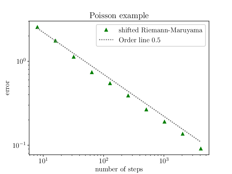
We close this section with a short numerical experiment. Hereby we applied the randomly shifted Riemann–Maruyama quadrature rule for the approximation of an Itô-integral whose integrand is a Poisson process. For the error plot displayed in Figure 2 we chose the final time $T=10$ and the intensity parameter $a=\frac{3}{4}$ . As step sizes we took $h\in\{T\,2^{-i}\,:\,i=3,\ldots,11\}$ . For the approximation of the error we compared the result of the quadrature rule with a given step size $h$ to a numerical reference solution with the smaller step size $\frac{h}{16}$ driven by the same stochastic trajectories. In addition, the $L^{2}(\Omega)$ -norm was approximated by a standard Monte Carlo simulation with $2000$ independent samples.

As one can see in Figure 2, the randomly shifted Riemann–Maruyama rule performed as expected with an experimental order of convergence close to $\frac{1}{2}$ , in agreement with the regularity of the Poisson process. Since we already knew from Section 5 that the higher order quadrature rule (8) does not yield an advantage if the integrand has jumps, it was not implemented in this example. In Table 2 we also show the numerical values of the computed errors and corresponding asymptotically valid $95\%$ -confidence intervals based on the central limit theorem. Apparently, already with just $2000$ Monte Carlo samples the variance of the error estimator is quite decent.

Acknowledgement

The authors wish to express their gratitude to Stefan Heinrich for many interesting discussions on this topic. This research was carried out in the framework of Matheon supported by Einstein Foundation Berlin. The second named author also gratefully acknowledges financial support by the German Research Foundation through the research unit FOR 2402 – Rough paths, stochastic partial differential equations and related topics – at TU Berlin.

References

[1] D. L. Burkholder. Martingale transforms. Ann. Math. Statist., 37:1494–1504, 1966.
[2] T. Daun and S. Heinrich. Complexity of Banach space valued and parametric stochastic Itô integration. J. Complexity, 40:100–122, 2017.
[3] F. Demengel and G. Demengel. Functional Spaces for the Theory of Elliptic Partial Differential Equations. Universitext. Springer, London; EDP Sciences, Les Ulis, 2012. Translated from the 2007 French original by Reinie Erné.
[4] E. Di Nezza, G. Palatucci, and E. Valdinoci. Hitchhiker’s guide to the fractional Sobolev spaces. Bull. Sci. Math., 136(5):521–573, 2012.
[5] C. Geiss and S. Geiss. On an approximation problem for stochastic integrals where random time nets do not help. Stochastic Process. Appl., 116(3):407–422, 2006.
[6] P. Glasserman. Monte Carlo Methods in Financial Engineering, volume 53 of Applications of Mathematics. Springer-Verlag, New York, 2004. Stochastic Modelling and Applied Probability.
[7] S. Heinrich. Lower complexity bounds for parametric stochastic Itô integration. Preprint, 2017.
[8] O. Kallenberg. Foundations of Modern Probability. Probability and its Applications. Springer-Verlag, New York, second edition, 2002.
[9] A. Klenke. Probability Theory. Universitext. Springer, London, second edition, 2014. A comprehensive course.
[10] P. E. Kloeden and E. Platen. Numerical Solution of Stochastic Differential Equations. Springer, Berlin, third edition, 1999.
[11] X. Mao. Stochastic Differential Equations and Applications. Horwood Publishing Limited, Chichester, second edition, 2008.
[12] G. N. Milstein and M. V. Tretyakov. Stochastic Numerics for Mathematical Physics. Scientific Computation. Springer-Verlag, Berlin, 2004.
[13] S. Peszat and J. Zabczyk. Stochastic Partial Differential Equations with Lévy Noise, volume 113 of Encyclopedia of Mathematics and its Applications. Cambridge University Press, Cambridge, 2007.
[14] P. Przybyłowicz. Linear information for approximation of the Itô integrals. Numer. Algorithms, 52(4):677–699, 2009.
[15] P. Przybyłowicz. Adaptive Itô-Taylor algorithm can optimally approximate the Itô integrals of singular functions. J. Comput. Appl. Math., 235(1):203–217, 2010.
[16] P. Przybyłowicz. Minimal asymptotic error for one-point approximation of SDEs with time-irregular coefficients. J. Comput. Appl. Math., 282:98–110, 2015.
[17] A. Rößler. Explicit order 1.5 schemes for the strong approximation of Itô stochastic differential equations. PAMM, 5(1):817–818, 2005.
[18] J. Simon. Sobolev, Besov and Nikolskiĭ fractional spaces: imbeddings and comparisons for vector valued spaces on an interval. Ann. Mat. Pura Appl. (4), 157:117–148, 1990.
[19] G. W. Wasilkowski and H. Woźniakowski. On the complexity of stochastic integration. Math. Comp., 70(234):685–698, 2001.

	$\displaystyle{\mathbb{E}}_{W}\Big[E^{n}_{\theta}\Big\|{\mathcal{F}}^{W}_{\theta_{m}}\Big]$	$\displaystyle={\mathbb{E}}_{W}\Big[\int_{0}^{\theta_{1}}G(t)\,\mathrm{d}W(t)+\sum_{j=1}^{n-1}\int_{\theta_{j}}^{\theta_{j+1}}\big(G(t)-G(\theta_{j})\big)\,\mathrm{d}W(t)\Big\|{\mathcal{F}}^{W}_{\theta_{m}}\Big]$
		$\displaystyle=\int_{0}^{\theta_{1}}G(t)\,\mathrm{d}W(t)+\sum_{j=1}^{m-1}\int_{\theta_{j}}^{\theta_{j+1}}\big(G(t)-G(\theta_{j})\big)\,\mathrm{d}W(t)$
		$\displaystyle\quad+{\mathbb{E}}_{W}\Big[\sum_{j=m}^{n-1}\int_{\theta_{j}}^{\theta_{j+1}}\big(G(t)-G(\theta_{j})\big)\,\mathrm{d}W(t)\Big\|{\mathcal{F}}^{W}_{\theta_{m}}\Big]=E^{m}_{\theta},$

		$\displaystyle\Big({\mathbb{E}}_{W}\Big[\big\|E^{N+1}_{\theta}\big\|^{p}\Big]\Big)^{\frac{1}{p}}$
		$\displaystyle\quad\leq C_{p}\Big({\mathbb{E}}_{W}\Big[\Big(\big\|E^{1}_{\theta}\big\|^{2}+\sum_{j=1}^{N}\big\|E^{j+1}_{\theta}-E^{j}_{\theta}\big\|^{2}\Big)^{\frac{p}{2}}\Big]\Big)^{\frac{1}{p}}$
		$\displaystyle\quad=C_{p}\Big(\Big\\|\big\|E^{1}_{\theta}\big\|^{2}+\sum_{j=1}^{N}\big\|E^{j+1}_{\theta}-E^{j}_{\theta}\big\|^{2}\Big\\|_{L^{\frac{p}{2}}(\Omega_{W})}\Big)^{\frac{1}{2}}$
		$\displaystyle\quad\leq C_{p}\Big(\big\\|E^{1}_{\theta}\big\\|^{2}_{L^{p}(\Omega_{W})}+\sum_{j=1}^{N}\big\\|E^{j+1}_{\theta}-E^{j}_{\theta}\big\\|^{2}_{L^{p}(\Omega_{W})}\Big)^{\frac{1}{2}}$
		$\displaystyle\quad\leq C_{p}\big\\|E^{1}_{\theta}\big\\|_{L^{p}(\Omega_{W})}+C_{p}\Big(\sum_{j=1}^{N}\big\\|E^{j+1}_{\theta}-E^{j}_{\theta}\big\\|^{2}_{L^{p}(\Omega_{W})}\Big)^{\frac{1}{2}}=:C_{p}\big(X_{1}+X_{2}\big),$

	$\displaystyle X_{2}^{2}$	$\displaystyle=\sum_{j=1}^{N}\big\\|E^{j+1}_{\theta}-E^{j}_{\theta}\big\\|^{2}_{L^{p}(\Omega_{W})}$
		$\displaystyle=\sum_{j=1}^{N}\Big\\|\int_{\theta_{j}}^{\theta_{j+1}}\big(G(t)-G(\theta_{j})\big)\,\mathrm{d}W(t)\Big\\|^{2}_{L^{p}(\Omega_{W})}$
		$\displaystyle\leq\frac{p(p-1)}{2}h^{\frac{p-2}{p}}\sum_{j=1}^{N}\Big(\int_{\theta_{j}}^{\theta_{j+1}}{\mathbb{E}}_{W}\big[\|G(t)-G(\theta_{j})\|^{p}\big]\,\mathrm{d}t\Big)^{\frac{2}{p}}.$

		$\displaystyle{\mathbb{E}}_{\Theta}\Big[\Big(\sum_{i=1}^{N}\Big(\int_{\Theta_{i}}^{\Theta_{i+1}}{\mathbb{E}}_{W}\big[\big\|G(t)-G(\Theta_{i})\big\|^{p}\big]\,\mathrm{d}t\Big)^{\frac{2}{p}}\Big)^{\frac{p}{2}}\Big]$
		$\displaystyle\quad\leq N^{\frac{p-2}{2}}\sum_{i=1}^{N}{\mathbb{E}}_{\Theta}\Big[\int_{\Theta_{i}}^{\Theta_{i+1}}{\mathbb{E}}_{W}\big[\big\|G(t)-G(\Theta_{i})\big\|^{p}\big]\,\mathrm{d}t\Big]$
		$\displaystyle\quad\leq N^{\frac{p-2}{2}}h^{1+p\sigma}\sum_{i=1}^{N}{\mathbb{E}}_{\Theta}\Big[\int_{\Theta_{i}}^{\Theta_{i+1}}\frac{{\mathbb{E}}_{W}\big[\big\|G(t)-G(\Theta_{i})\big\|^{p}\big]}{\|t-\Theta_{i}\|^{1+p\sigma}}\,\mathrm{d}t\Big]$
		$\displaystyle\quad\leq N^{\frac{p-2}{2}}h^{1+p\sigma}\sum_{i=1}^{N}\int_{0}^{T}{\mathbb{E}}_{\Theta}\Big[\frac{{\mathbb{E}}_{W}\big[\big\|G(t)-G(\Theta_{i})\big\|^{p}\big]}{\|t-\Theta_{i}\|^{1+p\sigma}}\Big]\,\mathrm{d}t$
		$\displaystyle\quad=N^{\frac{p-2}{2}}h^{1+p\sigma}\sum_{i=1}^{N}\int_{0}^{T}\frac{1}{h}\int_{t_{i-1}}^{t_{i}}\frac{{\mathbb{E}}_{W}\big[\big\|G(t)-G(s)\big\|^{p}\big]}{\|t-s\|^{1+p\sigma}}\,\mathrm{d}s\,\mathrm{d}t$
		$\displaystyle\quad\leq N^{\frac{p-2}{2}}h^{p\sigma}\\|G\\|_{L^{p}(\Omega_{W};W^{\sigma,p}(0,T))}^{p},$

		$\displaystyle\Big(\sum_{j=1}^{N}\Big\\|\int_{t_{j-1}}^{t_{j}}\int_{t_{j-1}}^{t_{j}}\int_{t_{j-\frac{1}{2}}}^{t}\big(\dot{g}(s)-\dot{g}(r)\big)\,\mathrm{d}s\,\mathrm{d}r\,\mathrm{d}W(t)\Big\\|_{L^{p}(\Omega_{W})}^{2}\Big)^{\frac{1}{2}}$
		$\displaystyle\quad\leq\Big(\frac{p(p-1)}{2}\Big)^{\frac{1}{2}}h^{\frac{p-2}{2p}}\Big(\sum_{j=1}^{N}\Big(\int_{t_{j-1}}^{t_{j}}\Big\|\int_{t_{j-1}}^{t_{j}}\int_{t_{j-\frac{1}{2}}}^{t}\big(\dot{g}(s)-\dot{g}(r)\big)\,\mathrm{d}s\,\mathrm{d}r\Big\|^{p}\,\mathrm{d}t\Big)^{\frac{2}{p}}\Big)^{\frac{1}{2}}$
		$\displaystyle\quad\leq\Big(\frac{p(p-1)}{2}\Big)^{\frac{1}{2}}h^{\frac{p-2}{2p}}N^{\frac{p-2}{2p}}\Big(\sum_{j=1}^{N}\int_{t_{j-1}}^{t_{j}}\Big\|\int_{t_{j-1}}^{t_{j}}\int_{t_{j-\frac{1}{2}}}^{t}\big(\dot{g}(s)-\dot{g}(r)\big)\,\mathrm{d}s\,\mathrm{d}r\Big\|^{p}\,\mathrm{d}t\Big)^{\frac{1}{p}}$
		$\displaystyle\quad\leq\Big(\frac{p(p-1)}{2}\Big)^{\frac{1}{2}}T^{\frac{p-2}{2p}}\Big(\sum_{j=1}^{N}h^{2(p-1)}\int_{t_{j-1}}^{t_{j}}\int_{t_{j-1}}^{t_{j}}\int_{t_{j-\frac{1}{2}}}^{t}\big\|\dot{g}(s)-\dot{g}(r)\big\|^{p}\,\mathrm{d}s\,\mathrm{d}r\,\mathrm{d}t\Big)^{\frac{1}{p}}$
		$\displaystyle\quad\leq\Big(\frac{p(p-1)}{2}\Big)^{\frac{1}{2}}T^{\frac{p-2}{2p}}\Big(\sum_{j=1}^{N}h^{2p+p\sigma}\int_{t_{j-1}}^{t_{j}}\int_{t_{j-1}}^{t_{j}}\frac{\big\|\dot{g}(s)-\dot{g}(r)\big\|^{p}}{\|s-r\|^{p\sigma+1}}\,\mathrm{d}s\,\mathrm{d}r\Big)^{\frac{1}{p}}$
		$\displaystyle\quad\leq\Big(\frac{p(p-1)}{2}\Big)^{\frac{1}{2}}T^{\frac{p-2}{2p}}h^{2+\sigma}\\|g\\|_{W^{1+\sigma,p}(0,T)},$