跳到论文正文
W Papers独立论文阅读器 arXiv:1712.07568 论文正文 计算阅读时间 · 0%
引用这篇论文根据当前论文元数据生成,正式投稿前建议核对。


License: arXiv.org perpetual non-exclusive license
arXiv:1712.07568v1 [math.PR] 20 Dec 2017

Mixing time of vertex-weighted exponential
random graphsThanks: Mei Yin’s research was partially supported by NSF grant DMS-1308333.

Ryan DeMuse and Terry Easlick and Mei Yin Address: Department of Mathematics, University of Denver, Denver, CO 80208, USA Email address: ryan.demuse@du.edu
terry.easlick@du.edu
mei.yin@du.edu
August 24, 2026
Abstract.

Exponential random graph models have become increasingly important in the study of modern networks ranging from social networks, economic networks, to biological networks. They seek to capture a wide variety of common network tendencies such as connectivity and reciprocity through local graph properties. Sampling from these exponential distributions is crucial for parameter estimation, hypothesis testing, as well as understanding the features of the network in question. We inspect the efficiency of a popular sampling technique, the Glauber dynamics, for vertex-weighted exponential random graphs. Letting nn be the number of vertices in the graph, we identify a region in the parameter space where the mixing time for the Glauber dynamics is Θ⁡(n​log⁡n)\Theta(n\log n) (the high temperature phase) and a complement region where the mixing time is exponentially slow on the order of eΩ⁡(n)e^{\Omega(n)} (the low temperature phase). Lastly, we give evidence that along a critical curve in the parameter space the mixing time is O⁡(n2/3)O(n^{2/3}).

Keywords Exponential random graphs ⋅\cdot Mixing time ⋅\cdot Glauber dynamics

Mathematics Subject Classification 05C80 ⋅\cdot 60J10 ⋅\cdot 90B15

1. Introduction

Exponential random graph models are powerful tools in the study of modern networks ranging from social networks, economic networks, to biological networks. By representing the complex global structure of a large network through tractable local properties, these models seek to capture a wide variety of common network tendencies. See for example Bollobás [4], Durrett [8], van der Hofstad [11], Newman [15], and references therein. Despite their flexibility, conventionally used exponential random graphs suffer from some deficiencies that may hamper their utility to researchers [7] [12]. Consider the dynamics of spreading events in a complex network. There are sensitive control points collectively known as “influential spreaders”, whose infection maximizes the overall fraction of infected vertices. For information diffusion over Twitter for example, the influential spreaders may be thought of as a celebrity or a news source. Vertices in the network thus carry with themselves some distinguishing features, a phenomenon that could not be directly modeled by standard exponential random graphs since their underlying probability space consists of simple graphs only. By placing weights on the vertices, the current work addresses this limitation of the exponential model.

Before proceeding further, we provide another reason why the vertex-weighted model may be of interest [2]. Let 𝒢n\mathcal{G}_{n} be the set of all vertex-weighted labeled graphs GnG_{n} on nn vertices. Assume that the vertex weights are iid real random variables subject to a common distribution ν\nu supported on [0,1][0,1], the edge weight between two vertices is a product of the vertex weights, and the triangle weight among three vertices is a product of the edge weights. Let UU be a random variable distributed according to ν\nu and denote its expectation with respect to ν\nu by 𝔼\mathbb{E}. Further denote the expected edge weight of Gn∈𝒢nG_{n}\in\mathcal{G}_{n} by ee and the expected triangle weight by tt. Then we have e=𝔼​(U)2e=\mathbb{E}(U)^{2} and t=(𝔼⁡(U2))3t=(\mathbb{E}(U^{2}))^{3}. Note that by suitably choosing ν\nu, the entire region between the upper boundary of the realizable edge-triangle densities and the Erdős-Rényi curve (e3≤t≤e3/2e^{3}\leq t\leq e^{3/2}) may be attained for vertex-weighted random graphs. See Figure 1. If we take UU to be Bernoulli, the upper boundary is reproduced:

𝔼⁡(U)≥𝔼⁡(U2)⟹e3/2≥t.\mathbb{E}(U)\geq\mathbb{E}(U^{2})\implies e^{3/2}\geq t. (1)

If we take UU to be a constant a.s., the Erdős-Rényi curve is recovered:

𝔼⁡(U2)≥𝔼​(U)2⟹t≥e3.\mathbb{E}(U^{2})\geq\mathbb{E}(U)^{2}\implies t\geq e^{3}. (2)

By contrast, since simple graphs may be interpreted as having iid Bernoulli(.5)(.5) weights on the edges, the underlying graph space of standard exponential random graphs lies at a single point (1/2,1/8)(1/2,1/8) on the Erdős-Rényi curve. Even without incorporating the exponential construction, assigning vertex weights alone adds intriguing characteristics to the model.

Refer to caption
Figure 1. The cyan region shows where the expected edge and triangle densities lie for a vertex-weighted random graph model.

1.1. The model

In this paper we will restrict our attention to vertex-weighted exponential random graph models where the vertex weights take values in 00 and 11 only. We include in the exponent a combination of edge and triangle densities, both with non-negative parameters. Even under this simplification, the vertex-weighted model depicts captivating behaviors in large-scale networks. Instead of Erdős-Rényi, it emphasizes the formation of cliques, and is particularly suited for the modeling of a broad range of social networks. Consider the Facebook friend graph for example, where we make the idealistic assumption that a person is either interested (vertex value 11) or not (vertex value 00) in building a friendship. Then having value 11 at three distinct vertices will force the formation of a triangle rather than a two-star, which is in analogy with the common conception that a friend of a friend is more likely to be a friend. An added benefit of this setting is that the model may be considered as an extension of the lattice gas (Ising) model on a graph, and the techniques of spin models may be employed in our investigation [9].

A graph Gn∈𝒢nG_{n}\in\mathcal{G}_{n} may be viewed as an element of X∈𝒳:={0,1}nX\in\mathcal{X}:=\{0,1\}^{n}, referred to as “configurations”, that attributes weights 00 or 11 to the ordered vertices of GnG_{n}. Denote by X⁡(i)X(i) the weight of vertex ii. Borrowing terminology from spin models, the vertex weight X⁡(i)X(i) will be called the “spin” at ii. By iid-ness, the spins at different vertices are independent, and subject to a common distribution ν\nu that assumes value 00 with probability 1−p1-p and 11 with probability pp for some p∈(0,1)p\in(0,1). Let H1H_{1} be the number of edges for the configuration XX and H2H_{2} be the number of triangles. They may be formulated explicitly in terms of lattice gas (Ising) spins:

H1​(X)=∑i≠jX⁡(i)​X​(j)​ and ​H2​(X)=∑i≠j≠kX⁡(i)​X​(j)​X​(k),H_{1}(X)=\sum_{i\neq j}X(i)X(j)\text{ and }H_{2}(X)=\sum_{i\neq j\neq k}X(i)X(j)X(k), (3)

where the inequality n1≠n2≠⋯≠nkn_{1}\neq n_{2}\neq\cdots\neq n_{k} means that ni≠njn_{i}\neq n_{j} for any i≠ji\neq j. We rescale the edge and triangle parameters in the exponent, H=(α1/n)​H1+(α2/n2)​H2H=(\alpha_{1}/n)H_{1}+(\alpha_{2}/n^{2})H_{2}, so that the total contribution of a single vertex to the weights is O⁡(1)O(1). We are now ready to introduce a Gibbs distribution to the set of spin configurations 𝒳\mathcal{X}. To avoid cumbersome notation, we suppress the nn-dependence in many of the quantities under discussion.

Definition 1.

Take α1≥0\alpha_{1}\geq 0, α2≥0\alpha_{2}\geq 0, and p∈(0,1)p\in(0,1). Let X∈𝒳X\in\mathcal{X} be a spin configuration. Denote by ω⁡(X)\omega(X) the number of vertices with spin 11 in XX. Assign a Gibbs probability measure on 𝒳\mathcal{X} as

π⁡(X)=Z−1​exp⁡(H⁡(X))​pω⁡(X)​(1−p)n−ω⁡(X),\pi(X)=Z^{-1}\exp(H(X))p^{\omega(X)}(1-p)^{n-\omega(X)}, (4)

where H=(α1/n)​H1+(α2/n2)​H2H=(\alpha_{1}/n)H_{1}+(\alpha_{2}/n^{2})H_{2} is the combination of edge and triangle weights and Z=Z⁡(n,p,α1,α2)Z=Z(n,p,\alpha_{1},\alpha_{2}) is the normalizing constant (partition function).

The configuration space 𝒳\mathcal{X} can be partially ordered in the sense that for X,Y∈𝒳X,Y\in\mathcal{X}, we say that X≤YX\leq Y if and only if X⁡(i)≤Y⁡(i)X(i)\leq Y(i) for every i∈{1,…,n}i\in\{1,\dots,n\}. To model the evolution of the network towards equilibrium, we will adopt (single-site) Glauber dynamics, which is a discrete-time irreducible and aperiodic Markov chain (Xt)t=0∞\left(X_{t}\right)_{t=0}^{\infty} on 𝒳\mathcal{X}. Under the Glauber dynamics, the random graph evolves by selecting a vertex ii at random and updating the spin X⁡(i)X(i) according to π\pi conditioned to agree with the spins at all vertices not equal to ii. By sampling from the exponential distribution using Glauber dynamics, we learn the global structure of the network as well as parameters describing the interactions. Explicitly, let X∈𝒳X\in\mathcal{X} be a configuration and set the initial state X0=XX_{0}=X. The next step of the Markov chain, X1X_{1}, is obtained as follows. Choose a vertex ii uniformly at random from {1,…,n}\{1,\dots,n\}. Let X1​(j)=X​(j)X_{1}(j)=X(j) for all j≠ij\neq i, X1​(i)=1X_{1}(i)=1 with probability P+P_{+} and X1​(i)=0X_{1}(i)=0 with probability P−P_{-}, where the update probabilities P+P_{+} and P−P_{-} are given by

P+​(X,i)=p​exp⁡(H′​(X,i))p​exp⁡(H′​(X,i))+(1−p)P_{+}(X,i)=\frac{p\exp(H^{\prime}(X,i))}{p\exp(H^{\prime}(X,i))+(1-p)} (5)

and

P−​(X,i)=1−pp​exp⁡(H′​(X,i))+(1−p).P_{-}(X,i)=\frac{1-p}{p\exp(H^{\prime}(X,i))+(1-p)}. (6)

Here H′=(α1/n)​S+(α2/n2)​TH^{\prime}=(\alpha_{1}/n)S+(\alpha_{2}/n^{2})T depends only on the spins at vertices other than ii, with

S⁡(X,i)=∑i≠jX⁡(j)​ and ​T​(X,i)=∑i≠j≠kX⁡(j)​X​(k)=S​(X,i)​(S​(X,i)−1)2.S(X,i)=\sum_{i\neq j}X(j)\text{ and }T(X,i)=\sum_{i\neq j\neq k}X(j)X(k)=\frac{S(X,i)(S(X,i)-1)}{2}. (7)

For X,Y∈𝒳X,Y\in\mathcal{X}, the transition matrix for the Glauber dynamics is then

P⁡(X,Y)=1n​∑if⁡(Y⁡(i))​exp⁡(Y⁡(i)​H′​(X,i))f⁡(Y⁡(i))​exp⁡(Y⁡(i)​H′​(X,i))+f⁡(1−Y⁡(i))​exp⁡((1−Y⁡(i))​H′​(X,i))​𝟏{Y⁡(j)=X⁡(j)j≠i},P(X,Y)=\frac{1}{n}\sum_{i}\frac{f(Y(i))\exp\left(Y(i)H^{\prime}(X,i)\right)}{f(Y(i))\exp\left(Y(i)H^{\prime}(X,i)\right)+f(1-Y(i))\exp\left((1-Y(i))H^{\prime}(X,i)\right)}\mathbf{1}_{\left\{\begin{subarray}{c}Y(j)=X(j)\\ j\neq i\end{subarray}\right\}}, (8)

where Y⁡(i)∈{0,1}Y(i)\in\{0,1\} and we define ff such that f⁡(0)=1−pf(0)=1-p and f⁡(1)=pf(1)=p to lighten the notation.

1.2. Mixing time

The Gibbs distribution π\pi is stationary and reversible for the Glauber dynamics chain. By the convergence theorem for ergodic Markov chains, the Glauber dynamics will converge to the stationary distribution and our goal is to obtain some estimates on the mixing time, since it greatly affects the efficiency of simulation studies and sampling algorithms [3] [6]. Given ε>0\varepsilon>0, the mixing time for this Markov chain is defined as

tmix​(ε):=min⁡{t:d⁡(t)≤ε},t_{\text{mix}}(\varepsilon):=\min\{t:d(t)\leq\varepsilon\}, (9)

where

d⁡(t)=maxX∈𝒳⁡‖Pt​(X,⋅)−π‖TVd(t)=\max_{X\in\mathcal{X}}\left\lVert P^{t}(X,{\cdot})-\pi\right\rVert_{\text{TV}} (10)

measures the total variation distance to stationarity of the Glauber dynamics chain after tt steps. As is standard, we take tmix:=tmix​(1/4)t_{\text{mix}}:=t_{\text{mix}}(1/4). The mixing time is thus defined to be the minimum number of discrete time steps such that, starting from an arbitrary configuration XX, the chain is within total variation distance 1/41/4 from the stationary distribution π\pi. For background on mixing times, see Aldous and Fill [1] and Levin et al. [14]. Our results will indicate that the mixing time can vary enormously depending on the choice of parameters.

1.3. Normalized magnetization

Given a spin configuration X∈𝒳X\in\mathcal{X}, the normalized magnetization cc of XX is defined as

c⁡(X)=1n​∑i=1nX⁡(i).c(X)=\frac{1}{n}\sum_{i=1}^{n}X(i). (11)

Adopting (single-site) Glauber dynamics on 𝒳\mathcal{X}, the normalized magnetization chain (ct)t=0∞\left(c_{t}\right)_{t=0}^{\infty} is a projection of the chain (Xt)t=0∞\left(X_{t}\right)_{t=0}^{\infty} and so is also aperiodic and irreducible. Set the initial state c0=cc_{0}=c. From the mechanism described in Section 1.1, after one Glauber update, c1c_{1} will take on one of three values: c−1/nc-1/n, cc, or c+1/nc+1/n. If a spin 00 vertex is chosen and updated to spin 11, cc changes to c+1/nc+1/n. Alternatively, if a spin 11 vertex is chosen and updated to spin 00, cc changes to c−1/nc-1/n. When no spins are updated, cc stays the same. By (5), the probability that we select a spin 00 vertex and update it to spin 11 is

Pu=n−c​nn​p​exp⁡(α1​c+α22​c​(c−1n))p​exp⁡(α1​c+α22​c​(c−1n))+(1−p).P_{u}=\frac{n-cn}{n}\frac{p\exp\left(\alpha_{1}c+\frac{\alpha_{2}}{2}c(c-\frac{1}{n})\right)}{p\exp\left(\alpha_{1}c+\frac{\alpha_{2}}{2}c(c-\frac{1}{n})\right)+(1-p)}. (12)

Similarly, by (6), the probability that we select a spin 11 vertex and update it to spin 00 is

Pd=c​nn​1−pp​exp⁡(α1​(c−1n)+α22​(c−2n)​(c−1n))+(1−p).P_{d}=\frac{cn}{n}\frac{1-p}{p\exp\left(\alpha_{1}(c-\frac{1}{n})+\frac{\alpha_{2}}{2}(c-\frac{2}{n})(c-\frac{1}{n})\right)+(1-p)}. (13)

Combining (12) and (13), the magnetization ctc_{t} moves up with probability PuP_{u}, down with probability PdP_{d}, and remains unchanged with probability 1−Pu−Pd1-P_{u}-P_{d}. For nn large enough, Pu≍(1−c)​λ​(c)P_{u}\asymp(1-c)\lambda(c) and Pd≍c⁡(1−λ⁡(c))P_{d}\asymp c(1-\lambda(c)), where

λ⁡(c)=p​exp⁡(α1​c+α22​c2)p​exp⁡(α1​c+α22​c2)+(1−p)\lambda(c)=\frac{p\exp\left(\alpha_{1}c+\frac{\alpha_{2}}{2}c^{2}\right)}{p\exp\left(\alpha_{1}c+\frac{\alpha_{2}}{2}c^{2}\right)+(1-p)} (14)

represents the asymptotic probability that a chosen vertex is updated to spin 11. This implies that the expected magnetization drift is asymptotically (λ⁡(c)−c)/n(\lambda(c)-c)/n, and a rigorous justification may be found in Lemma 2.
Refer to caption
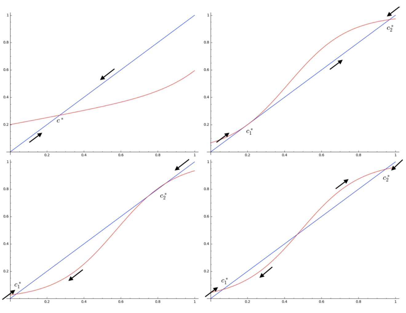
Figure 2. Behavior of the λ\lambda function in different regions of the parameter space with arrows indicating whether the fixed point is an attractor or a repellor.

1.4. Phase classification

The magnetization chain (ct)\left(c_{t}\right) is a deciding factor in the convergence of the Glauber dynamics chain (Xt)\left(X_{t}\right). Note that 0≤ct≤10\leq c_{t}\leq 1 and λ\lambda is a smooth and increasing function on [0,1][0,1]. Since λ⁡(0)>0\lambda(0)>0 and λ⁡(1)<1\lambda(1)<1, λ⁡(c)=c\lambda(c)=c admits at least one solution in (0,1)(0,1). If the solution cc is unique and not an inflection point, i.e. λ′​(c)<1\lambda^{\prime}(c)<1 (referred to as the “high temperature phase”), then independent of the initial position all configurations will be driven towards it, and the burn-in stage will cost O⁡(n)O(n) steps. See the upper left plot of Figure 2. Conversely, if there exist at least two solutions cc such that λ′​(c)<1\lambda^{\prime}(c)<1 (referred to as the “low temperature phase”), then the burn-in procedure will take the configurations to different attractor states depending on their initial positions. See the lower right plot of Figure 2. Once the configuration is close to an attractor, the Glauber dynamics allows an exponentially small flow of probability for it to leave. A detailed examination of the burn-in period will be provided in Section 2.

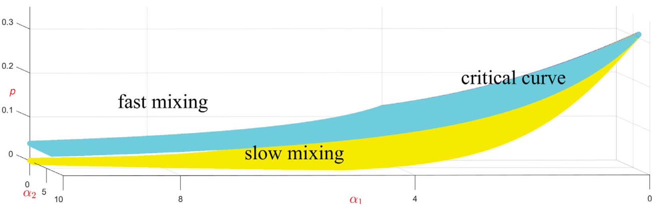
In Section 3, through estimating the average distance after one update between two coupled configurations that agree everywhere except at a single vertex, we show that the Glauber dynamics XtX_{t} mixes in O⁡(n​log⁡n)O(n\log n) steps in the high temperature phase. Relating to coupon collecting and employing spectral methods, the same asymptotic lower bound Ω⁡(n​log⁡n)\Omega(n\log n) is validated. While in Section 4, by a conductance argument using the Cheeger inequality, we establish exponentially slow mixing of the Glauber dynamics XtX_{t} in the low temperature phase. Finally, in Section 5, we give evidence that the burn-in will cost O⁡(n3/2)O(n^{3/2}) steps along the “critical curve”, and the Glauber dynamics XtX_{t} is thus expected to mix in O⁡(n3/2)O(n^{3/2}) steps. See Figure 3. The cyan and yellow surfaces separate the high and low temperature phases, with their intersection marked by the critical curve. Convergence of the Glauber dynamics XtX_{t} elsewhere on the two surfaces corresponds to the situation where λ⁡(c)=c\lambda(c)=c has at least two solutions and one solution cc satisfies λ′​(c)=1\lambda^{\prime}(c)=1. See the upper and right and lower left plots of Figure 2. The mixing time largely depends on the movement of the chain around the inflection point and is not addressed in this paper.
Refer to caption
Figure 3. Surfaces in the parameter space illustrating the region with fast vs. slow mixing and identifying the critical curve.

2. Burn-in period

We start by running the Glauber dynamics for an initial burn-in period. This will ensure that the associated magnetization chain is with high probability close to an attractor. Let X∈𝒳X\in\mathcal{X} be any spin configuration. Set the initial state X0=XX_{0}=X and let ctc_{t} be the normalized magnetization of XtX_{t} at time tt. We use ℙX\mathbb{P}_{X} and 𝔼X\mathbb{E}_{X} respectively to denote the underlying probability measure and associated expectation. To keep the notation light, we omit the explicit dependence on XX when it is clear from the context.

Lemma 2.

The expected drift in ctc_{t} after one step of the Glauber dynamics, starting from the configuration XX, is given by

𝔼⁡(ct+1−ct∣ct)=1n​(λ⁡(ct)−ct)+O⁡(1n2),\mathbb{E}(c_{t+1}-c_{t}\mid c_{t})=\frac{1}{n}\left(\lambda(c_{t})-c_{t}\right)+O\left(\frac{1}{n^{2}}\right), (15)

where λ\lambda is defined as in (14).

Proof.

From our discussion in Section 1.3, we compute

𝔼⁡(ct+1−ct∣ct)\displaystyle\mathbb{E}(c_{t+1}-c_{t}\mid c_{t}) =1n​(1−ct)​p​exp⁡(α1​ct+α22​ct​(ct−1n))p​exp⁡(α1​ct+α22​ct​(ct−1n))+(1−p)\displaystyle=\frac{1}{n}(1-c_{t})\frac{p\exp\left(\alpha_{1}c_{t}+\frac{\alpha_{2}}{2}c_{t}\left(c_{t}-\frac{1}{n}\right)\right)}{p\exp\left(\alpha_{1}c_{t}+\frac{\alpha_{2}}{2}c_{t}\left(c_{t}-\frac{1}{n}\right)\right)+(1-p)}
−1n​ct​1−pp​exp⁡(α1​(ct−1n)+α22​(ct−1n)​(ct−2n))+(1−p).\displaystyle\hskip 28.45274pt-\frac{1}{n}c_{t}\frac{1-p}{p\exp\left(\alpha_{1}\left(c_{t}-\frac{1}{n}\right)+\frac{\alpha_{2}}{2}\left(c_{t}-\frac{1}{n}\right)\left(c_{t}-\frac{2}{n}\right)\right)+(1-p)}. (16)

Note that lower order fluctuations may be extracted from the exponents:

exp⁡(α1​ct+α22​ct​(ct−1n))=exp⁡(−α22​n​ct)​exp⁡(α1​ct+α22​(ct)2),\exp\left(\alpha_{1}c_{t}+\frac{\alpha_{2}}{2}c_{t}\left(c_{t}-\frac{1}{n}\right)\right)=\exp\left(-\frac{\alpha_{2}}{2n}c_{t}\right)\exp\left(\alpha_{1}c_{t}+\frac{\alpha_{2}}{2}\left(c_{t}\right)^{2}\right), (17)
exp⁡(α1​(ct−1n)+α22​(ct−1n)​(ct−2n))=exp⁡(−α1n−3​α22​n​ct+α2n2)​exp⁡(α1​ct+α22​(ct)2),\exp\left(\alpha_{1}\left(c_{t}-\frac{1}{n}\right)+\frac{\alpha_{2}}{2}\left(c_{t}-\frac{1}{n}\right)\left(c_{t}-\frac{2}{n}\right)\right)\\ =\exp\left(-\frac{\alpha_{1}}{n}-\frac{3\alpha_{2}}{2n}c_{t}+\frac{\alpha_{2}}{n^{2}}\right)\exp\left(\alpha_{1}c_{t}+\frac{\alpha_{2}}{2}\left(c_{t}\right)^{2}\right), (18)

which gives

𝔼⁡(ct+1−ct∣ct)\displaystyle\mathbb{E}(c_{t+1}-c_{t}\mid c_{t}) =1n​(λ⁡(ct)−ct)\displaystyle=\frac{1}{n}\left(\lambda(c_{t})-c_{t}\right)
+λ⁡(ct)n​(1−ct)​exp⁡(−α22​n​ct)−11+(p1−p)​exp⁡(−α22​n​ct)​exp⁡(α1​ct+α22​(ct)2)\displaystyle+\frac{\lambda(c_{t})}{n}(1-c_{t})\frac{\exp\left(-\frac{\alpha_{2}}{2n}c_{t}\right)-1}{1+\left(\frac{p}{1-p}\right)\exp\left(-\frac{\alpha_{2}}{2n}c_{t}\right)\exp\left(\alpha_{1}c_{t}+\frac{\alpha_{2}}{2}\left(c_{t}\right)^{2}\right)}
+λ⁡(ct)n​ct​exp⁡(−α1n−3​α22​n​ct+α2n2)−11+(p1−p)​exp⁡(−α1n−3​α22​n​ct+α2n2)​exp⁡(α1​ct+α22​(ct)2).\displaystyle+\frac{\lambda(c_{t})}{n}c_{t}\frac{\exp\left(-\frac{\alpha_{1}}{n}-\frac{3\alpha_{2}}{2n}c_{t}+\frac{\alpha_{2}}{n^{2}}\right)-1}{1+\left(\frac{p}{1-p}\right)\exp\left(-\frac{\alpha_{1}}{n}-\frac{3\alpha_{2}}{2n}c_{t}+\frac{\alpha_{2}}{n^{2}}\right)\exp\left(\alpha_{1}c_{t}+\frac{\alpha_{2}}{2}\left(c_{t}\right)^{2}\right)}. (19)

Following standard analytical argument, the long fractional terms above are O⁡(1/n)O(1/n). The conclusion readily follows. ∎

Applying Lemma 2, the following Theorem 3 and Corollaries 4 and 5 show that if the associated magnetization c0c_{0} of the initial configuration is significantly different from an attractor c∗c^{*} but bounded away from any other solution of the fixed point equation λ⁡(c)=c\lambda(c)=c, then there is a drift of the Glauber dynamics towards a configuration whose normalized magnetization is closer to c∗c^{*} than the starting state, i.e. ct→c∗c_{t}\rightarrow c^{*}. Theorem 3 is proved when c0>c∗c_{0}>c^{*}, and an analogous result holds for c0<c∗c_{0}<c^{*} using a similar line of reasoning. See Figure 2 for an illustration of this burn-in procedure.

Theorem 3.

Suppose λ⁡(c∗)=c∗\lambda(c^{\ast})=c^{\ast} and λ′​(c∗)<1\lambda^{\prime}(c^{\ast})<1. Let c¯>c∗\overline{c}>c^{\ast} be the smallest value satisfying λ⁡(c¯)=c¯\lambda(\overline{c})=\overline{c}. (If no such c¯\overline{c} exists, take c¯=1\overline{c}=1.) Let the initial magnetization be c0c_{0} with c∗+μ<c0<c¯−μc^{\ast}+\mu<c_{0}<\overline{c}-\mu for some μ>0\mu>0. Then there exist η,d>0\eta,d>0 depending only on μ,p,α1,α2\mu,p,\alpha_{1},\alpha_{2} such that T=d​nT=dn and

ℙ⁡(cT≤c0−η)≥1−e−Ω⁡(n).\mathbb{P}\left(c_{T}\leq c_{0}-\eta\right)\geq 1-e^{-\Omega(\sqrt{n})}. (20)
Proof.

Since λ′​(c∗)<1\lambda^{\prime}(c^{\ast})<1, λ⁡(c)−c<0\lambda(c)-c<0 for c∈[c∗+μ,c¯−μ]c\in[c^{\ast}+\mu,\overline{c}-\mu]. By the extreme value theorem, the maximum of the smooth function λ⁡(c)−c\lambda(c)-c is attained for some value c¯\underline{c} in the compact interval [c∗+μ,c¯−μ][c^{\ast}+\mu,\overline{c}-\mu]. Define γ>0\gamma>0 as γ=−(λ(c¯)−c¯)/2\gamma=-(\lambda(\underline{c})-\underline{c})/2. Choose η>0\eta>0 so that [c0−2​η,c0+η]⊆[c∗+μ,c¯−μ][c_{0}-2\eta,c_{0}+\eta]\subseteq[c^{\ast}+\mu,\overline{c}-\mu]. Let

Dt​(η)={ct:c0−2​η≤ct≤c0+η}.D_{t}(\eta)=\left\{c_{t}:c_{0}-2\eta\leq c_{t}\leq c_{0}+\eta\right\}. (21)

By Lemma 2, for ct∈Dt​(η)c_{t}\in D_{t}(\eta) and nn sufficiently large, 𝔼(ct+1−ct∣ct)≤−γ/n\mathbb{E}(c_{t+1}-c_{t}\mid c_{t})\leq-\gamma/n. Utilizing the negative drift −γ/n-\gamma/n of the biased random walk ctc_{t} and employing a moment generating function method, we first show that “bad” magnetization, i.e. ct>c0+ηc_{t}>c_{0}+\eta for some 0≤t≤T0\leq t\leq T, occurs with exponentially small probability.

Define St1,t2S_{t_{1},t_{2}} as

St1,t2=∑t=t1+1t2(ct−ct−1+γ2​n)​𝟏Dt−1.S_{t_{1},t_{2}}=\sum_{t=t_{1}+1}^{t_{2}}\left(c_{t}-c_{t-1}+\frac{\gamma}{2n}\right)\mathbf{1}_{D_{t-1}}. (22)

The random variable St1,t2S_{t_{1},t_{2}} records the change in “good” magnetization ctc_{t} from t1t_{1} to t2t_{2}, shifted by γ/(2​n)\gamma/(2n) per time step. Let ℱt\mathcal{F}_{t} be the natural filtration. By the tower property of expectation,

𝔼⁡(eθ​St1,t2)=𝔼⁡(eθ​St1,t2−1​𝔼​(eθ⁡(ct2−ct2−1+γ2​n)​𝟏Dt2−1∣ℱt2−1)).\displaystyle\mathbb{E}\left(e^{\theta S_{t_{1},t_{2}}}\right)=\mathbb{E}\left(e^{\theta S_{t_{1},t_{2}-1}}\mathbb{E}\left(e^{\theta(c_{t_{2}}-c_{t_{2}-1}+\frac{\gamma}{2n})\mathbf{1}_{D_{t_{2}-1}}}\mid\mathcal{F}_{t_{2}-1}\right)\right). (23)

Using linearity of expectation, we write

𝔼⁡(eθ⁡(ct2−ct2−1+γ2​n)​𝟏Dt2−1∣ℱt2−1)\displaystyle\mathbb{E}\left(e^{\theta(c_{t_{2}}-c_{t_{2}-1}+\frac{\gamma}{2n})\mathbf{1}_{D_{t_{2}-1}}}\mid\mathcal{F}_{t_{2}-1}\right)
=∑k=0∞𝔼⁡(θk​(ct2−ct2−1+γ2​n)kk!​𝟏Dt2−1k∣ℱt2−1)\displaystyle=\sum_{k=0}^{\infty}\mathbb{E}\left(\frac{\theta^{k}(c_{t_{2}}-c_{t_{2}-1}+\frac{\gamma}{2n})^{k}}{k!}\mathbf{1}_{D_{t_{2}-1}}^{k}\mid\mathcal{F}_{t_{2}-1}\right)
=1+𝔼⁡(θ⁡(ct2−ct2−1+γ2​n)​𝟏Dt2−1∣ℱt2−1)+∑k=2∞𝔼⁡(θk​(ct2−ct2−1+γ2​n)kk!​𝟏Dt2−1k∣ℱt2−1).\displaystyle=1+\mathbb{E}\left(\theta(c_{t_{2}}-c_{t_{2}-1}+\frac{\gamma}{2n})\mathbf{1}_{D_{t_{2}-1}}\mid\mathcal{F}_{t_{2}-1}\right)+\sum_{k=2}^{\infty}\mathbb{E}\left(\frac{\theta^{k}(c_{t_{2}}-c_{t_{2}-1}+\frac{\gamma}{2n})^{k}}{k!}\mathbf{1}_{D_{t_{2}-1}}^{k}\mid\mathcal{F}_{t_{2}-1}\right). (24)

Recall that 𝔼(ct+1−ct∣ct)≤−γ/n\mathbb{E}(c_{t+1}-c_{t}\mid c_{t})\leq-\gamma/n for ct∈Dtc_{t}\in D_{t}, and so

𝔼⁡(eθ⁡(ct2−ct2−1+γ2​n)​𝟏Dt2−1∣ℱt2−1)\displaystyle\mathbb{E}\left(e^{\theta(c_{t_{2}}-c_{t_{2}-1}+\frac{\gamma}{2n})\mathbf{1}_{D_{t_{2}-1}}}\mid\mathcal{F}_{t_{2}-1}\right) ≤1−γ​θ2​n​𝟏Dt2−1+O⁡(θ2n2).\displaystyle\leq 1-\frac{\gamma\theta}{2n}\mathbf{1}_{D_{t_{2}-1}}+O\left(\frac{\theta^{2}}{n^{2}}\right). (25)

Taking θ=c​n\theta=c\sqrt{n} for a sufficiently small constant cc, the above conditional expectation is less than 11. Iterating this procedure gives

𝔼⁡(eθ​St1,t2)≤𝔼⁡(eθ​St1,t2−1)≤⋯≤𝔼⁡(eθ​St1,t1)=1.\mathbb{E}\left(e^{\theta S_{t_{1},t_{2}}}\right)\leq\mathbb{E}\left(e^{\theta S_{t_{1},t_{2}-1}}\right)\leq{\cdots}\leq\mathbb{E}\left(e^{\theta S_{t_{1},t_{1}}}\right)=1. (26)

By the Chernoff bound,

ℙ⁡(St1,t2≥η2)≤𝔼⁡(eθ​St1,t2)eθ​η2=e−Ω⁡(n).\mathbb{P}\left(S_{t_{1},t_{2}}\geq\frac{\eta}{2}\right)\leq\frac{\mathbb{E}\left(e^{\theta S_{t_{1},t_{2}}}\right)}{e^{\theta\frac{\eta}{2}}}=e^{-\Omega(\sqrt{n})}. (27)

Consider the set

Bt1,t2(η)=(⋂t1≤t<t2Dt(η))⋂{ct2−ct1>η2},B_{t_{1},t_{2}}(\eta)=\left(\bigcap_{t_{1}\leq t<t_{2}}D_{t}(\eta)\right)\bigcap\left\{c_{t_{2}}-c_{t_{1}}>\frac{\eta}{2}\right\}, (28)

consisting of all “good” magnetizations at time t1t_{1} up to time t2t_{2}, with an increase of at least η/2\eta/2 from t1t_{1} to t2t_{2}. Subject to ct∈Dtc_{t}\in D_{t} for t1≤t<t2t_{1}\leq t<t_{2} and ct2−ct1>η/2c_{t_{2}}-c_{t_{1}}>\eta/2,

St1,t2\displaystyle S_{t_{1},t_{2}} =∑t=t1+1t2(ct−ct−1+γ2​n)\displaystyle=\sum_{t=t_{1}+1}^{t_{2}}\left(c_{t}-c_{t-1}+\frac{\gamma}{2n}\right)
=ct2−ct1+γ2​n​(t2−t1)>η2,\displaystyle=c_{t_{2}}-c_{t_{1}}+\frac{\gamma}{2n}(t_{2}-t_{1})>\frac{\eta}{2}, (29)

from which the containment Bt1,t2(η)⊆{St1,t2≥η/2}B_{t_{1},t_{2}}(\eta)\subseteq\{S_{t_{1},t_{2}}\geq\eta/2\} follows. Hence

ℙ⁡(⋃0≤t1<t2≤TBt1,t2)≤n2​e−Ω⁡(n)=e−Ω⁡(n).\mathbb{P}\left(\bigcup_{0\leq t_{1}<t_{2}\leq T}B_{t_{1},t_{2}}\right)\leq n^{2}e^{-\Omega(\sqrt{n})}=e^{-\Omega(\sqrt{n})}. (30)

Take nn large enough. Suppose ct>c0+ηc_{t}>c_{0}+\eta for some 0≤t≤T0\leq t\leq T. Then there exists a t1t_{1} such that c0−2​η≤csc_{0}-2\eta\leq c_{s} for all t1≤s≤tt_{1}\leq s\leq t. Define t2t_{2} to be the least time greater than t1t_{1} with ct2>c0+ηc_{t_{2}}>c_{0}+\eta. Then ct∈Dtc_{t}\in D_{t} for all t1≤t<t2t_{1}\leq t<t_{2} and ct2−ct1>η/2c_{t_{2}}-c_{t_{1}}>\eta/2. This implies that

{ct:ct>c0+η​ for some ​0≤t≤T}⊆⋃0≤t1<t2≤TBt1,t2,\left\{c_{t}:c_{t}>c_{0}+\eta\text{ for some }0\leq t\leq T\right\}\subseteq\bigcup_{0\leq t_{1}<t_{2}\leq T}B_{t_{1},t_{2}}, (31)

and further implies that

ℙ⁡(ct>c0+η​ for some ​0≤t≤T)≤e−Ω⁡(n).\mathbb{P}\left(c_{t}>c_{0}+\eta\text{ for some }0\leq t\leq T\right)\leq e^{-\Omega(\sqrt{n})}. (32)

We have thus shown that the normalized magnetization ctc_{t} remains below c0+ηc_{0}+\eta for all 0≤t≤T0\leq t\leq T with exponentially high probability, provided that c0c_{0} is suitably bounded away from any other fixed point of λ\lambda. Next we show that cTc_{T} ends below c0−ηc_{0}-\eta with exponentially high probability. We prove this by showing that ctc_{t} actually reaches c0−2​ηc_{0}-2\eta with exponentially high probability, and then by the preceding argument will have exponentially small probability of increasing to c0−ηc_{0}-\eta. We have

ℙ⁡(ct≥c0−2​η​ for all ​0≤t≤T)≤ℙ⁡(⋂0≤t≤TDt​(η))+ℙ⁡(ct>c0+η​ for some ​0≤t≤T).\mathbb{P}\left(c_{t}\geq c_{0}-2\eta\text{ for all }0\leq t\leq T\right)\leq\mathbb{P}\left(\bigcap_{0\leq t\leq T}D_{t}(\eta)\right)+\mathbb{P}\left(c_{t}>c_{0}+\eta\text{ for some }0\leq t\leq T\right). (33)

Subject to ct∈Dt​(η)c_{t}\in D_{t}(\eta) for 0≤t≤T0\leq t\leq T and noticing that at worst c0=1c_{0}=1 and cT=0c_{T}=0,

S0,T\displaystyle S_{0,T} =∑t=1T(ct−ct−1+γ2​n)​𝟏Dt−1\displaystyle=\sum_{t=1}^{T}\left(c_{t}-c_{t-1}+\frac{\gamma}{2n}\right)\mathbf{1}_{D_{t-1}}
=cT−c0+γ2​n​T≥−1+γ2​n​T.\displaystyle=c_{T}-c_{0}+\frac{\gamma}{2n}T\geq-1+\frac{\gamma}{2n}T. (34)

Using the Chernoff bound on S0,TS_{0,T} and assume that d>2/γd>2/\gamma,

ℙ⁡(ct≥c0−2​η​ for all ​0≤t≤T)≤ℙ⁡(S0,T≥−1+γ2​n​T)+e−Ω⁡(n)≤𝔼⁡(eθ​S0,T)eθ⁡(−1+γ2​n​T)+e−Ω⁡(n)=e−Ω⁡(n).\mathbb{P}\left(c_{t}\geq c_{0}-2\eta\text{ for all }0\leq t\leq T\right)\leq\mathbb{P}\left(S_{0,T}\geq-1+\frac{\gamma}{2n}T\right)+e^{-\Omega(\sqrt{n})}\\ \leq\frac{\mathbb{E}\left(e^{\theta S_{0,T}}\right)}{e^{\theta\left(-1+\frac{\gamma}{2n}T\right)}}+e^{-\Omega(\sqrt{n})}=e^{-\Omega(\sqrt{n})}. (35)

Finally,

ℙ⁡(cT≥c0−η)\displaystyle\mathbb{P}\left(c_{T}\geq c_{0}-\eta\right) ≤ℙ⁡(cT≥c0−η​ and ​ct<c0−2​η​ for some ​0≤t≤T)\displaystyle\leq\mathbb{P}\left(c_{T}\geq c_{0}-\eta\text{ and }c_{t}<c_{0}-2\eta\text{ for some }0\leq t\leq T\right)
+ℙ({ct≥c0−2η for all 0≤t≤T})≤e−Ω⁡(n),\displaystyle+\mathbb{P}\left(\left\{c_{t}\geq c_{0}-2\eta\text{ for all }0\leq t\leq T\right\}\right)\leq e^{-\Omega(\sqrt{n})}, (36)

where to bound the first probability on the right, we apply the bound on “bad” magnetization (32) with minor adaptation: initial magnetization ctc_{t} (for some 0≤t≤T0\leq t\leq T) in place of c0c_{0}, time interval under consideration [t,T][t,T] in place of [0,T][0,T], and the increase in magnetization c0−2​η→c0−ηc_{0}-2\eta\rightarrow c_{0}-\eta in place of c0→c0+ηc_{0}\rightarrow c_{0}+\eta. ∎

Repeated application of Theorem 3 shows that after a burn-in period on the order of O⁡(n)O(n), any suitably chosen configuration ends up close to an attractor c∗c^{\ast} with exponentially high probability. Recall the definition of high temperature phase and low temperature phase from Section 1.4. The following corollaries are immediate.

Corollary 4.

In the high temperature phase, suppose that c∗c^{\ast} is the unique solution to λ⁡(c)=c\lambda(c)=c and λ′​(c∗)<1\lambda^{\prime}(c^{\ast})<1. For any ε>0\varepsilon>0, there exists α>0\alpha>0 such that for any initial configuration with associated magnetization c0c_{0}, when t≥α​nt\geq\alpha n we have

ℙ⁡(ct≥c∗+ε)≤e−Ω⁡(n)\mathbb{P}\left(c_{t}\geq c^{\ast}+\varepsilon\right)\leq e^{-\Omega(\sqrt{n})} (37)

and

ℙ⁡(ct≤c∗−ε)≤e−Ω⁡(n).\mathbb{P}\left(c_{t}\leq c^{\ast}-\varepsilon\right)\leq e^{-\Omega(\sqrt{n})}. (38)
Corollary 5.

In the low temperature phase, suppose that c∗c^{\ast} is a solution to λ⁡(c)=c\lambda(c)=c and λ′​(c∗)<1\lambda^{\prime}(c^{\ast})<1. Take ε>0\varepsilon>0. If the associated magnetization c0c_{0} for some initial configuration satisfies c∗−ε≤c0≤c∗+εc^{\ast}-\varepsilon\leq c_{0}\leq c^{\ast}+\varepsilon, then there exists β>0\beta>0,

ℙ⁡(sup0<t<eβ​nct≥c∗+2​ε)≤e−Ω⁡(n)\mathbb{P}\left(\sup_{0<t<e^{\beta\sqrt{n}}}c_{t}\geq c^{\ast}+2\varepsilon\right)\leq e^{-\Omega(\sqrt{n})} (39)

and

ℙ⁡(inf0<t<eβ​nct≤c∗−2​ε)≤e−Ω⁡(n).\mathbb{P}\left(\inf_{0<t<e^{\beta\sqrt{n}}}c_{t}\leq c^{\ast}-2\varepsilon\right)\leq e^{-\Omega(\sqrt{n})}. (40)

3. Fast mixing at high temperature

In this section we study the mixing time of the Glauber dynamics in the high temperature phase. We first establish an upper bound O⁡(n​log⁡n)O(n\log n) using path coupling techniques of Bubley and Dyer [5]. Consider two arbitrary spin configurations X,Y∈𝒳X,Y\in\mathcal{X}. Taking “attractive” parameters αi≥0\alpha_{i}\geq 0 ensures that we may apply a monotone coupling on the chain (Xt,Yt)(X_{t},Y_{t}): XtX_{t} is a version of the Glauber dynamics with starting state XX and YtY_{t} is a version of the Glauber dynamics with starting state YY, if X0≤Y0X_{0}\leq Y_{0} then Xt≤YtX_{t}\leq Y_{t} for all tt. We write ℙX,Y\mathbb{P}_{X,Y} and 𝔼X,Y\mathbb{E}_{X,Y} for the underlying probability measure and associated expectation. To keep the notation light, we omit the explicit dependence on XX and YY when it is clear from the context. To understand how far apart XtX_{t} and YtY_{t} are, we introduce Hamming distance, which records the number of vertices where the two configurations disagree. Define ρ:𝒳×𝒳→{0,…,n}\rho:\mathcal{X}\times\mathcal{X}\to\{0,\dots,n\} by

ρ⁡(X,Y)=∑i=1n|X⁡(i)−Y⁡(i)|.\rho(X,Y)=\sum_{i=1}^{n}\left|X(i)-Y(i)\right|. (41)

Following standard contraction argument, it suffices to estimate the average distance after one Glauber update between two coupled configurations XX and YY with Hamming distance ρ⁡(X,Y)=1\rho(X,Y)=1.

Lemma 6.

Assume that sup0≤c≤1λ′​(c)<1\sup_{0\leq c\leq 1}\lambda^{\prime}(c)<1. Let X,Y∈𝒳X,Y\in\mathcal{X} be two spin configurations satisfying X≤YX\leq Y and ρ⁡(X,Y)=1\rho(X,Y)=1. Set the initial state X0=XX_{0}=X and Y0=YY_{0}=Y. Then there exists δ>0\delta>0 depending only on p,α1,α2p,\alpha_{1},\alpha_{2} such that a single step of the Glauber dynamics can be coupled when nn is sufficiently large:

𝔼(ρ(X1,Y1))≤e−δ/n.\mathbb{E}\left(\rho(X_{1},Y_{1})\right)\leq e^{-\delta/n}. (42)
Proof.

Let X,Y∈𝒳X,Y\in\mathcal{X} be two configurations such that X≤YX\leq Y and there exists a single vertex ii such that X⁡(i)=0X(i)=0 and Y⁡(i)=1Y(i)=1. Let UU be a uniform random variable on [0,1][0,1]. We apply the standard monotone coupling, where UU is used as the common source of noise to update both chains so that they agree as often as possible. From the mechanism described in Section 1.1, the chain evolves by selecting a vertex jj uniformly at random and updating the spin at jj. Set

X1​(j)={1U≤p+​(X,j),0U>p+​(X,j),Y1​(j)={1U≤p+​(Y,j),0U>p+​(Y,j),X_{1}(j)=\left\{\begin{array}[]{ll}1&U\leq p_{+}(X,j),\\ 0&U>p_{+}(X,j),\end{array}\right.\hskip 28.45274ptY_{1}(j)=\left\{\begin{array}[]{ll}1&U\leq p_{+}(Y,j),\\ 0&U>p_{+}(Y,j),\end{array}\right. (43)

and X1​(k)=X​(k)X_{1}(k)=X(k) and Y1​(k)=Y​(k)Y_{1}(k)=Y(k) for all k≠jk\neq j. Define the function f⁡(S)f(S) as

f⁡(S)=p​exp⁡(α1n​S+α22​n2​S​(S−1))p​exp⁡(α1n​S+α22​n2​S​(S−1))+(1−p).f(S)=\frac{p\exp\left(\frac{\alpha_{1}}{n}S+\frac{\alpha_{2}}{2n^{2}}S(S-1)\right)}{p\exp\left(\frac{\alpha_{1}}{n}S+\frac{\alpha_{2}}{2n^{2}}S(S-1)\right)+(1-p)}. (44)

If j=ij=i, then p+​(X,j)=f⁡(S⁡(X,j))=p+​(Y,j)p_{+}(X,j)=f\left(S(X,j)\right)=p_{+}(Y,j) and so ρ⁡(X1,Y1)=0\rho(X_{1},Y_{1})=0. For j≠ij\neq i, we have p+​(X,j)=f⁡(S⁡(X,j))p_{+}(X,j)=f\left(S(X,j)\right) while p+​(Y,j)=f⁡(S⁡(X,j)+1)p_{+}(Y,j)=f\left(S(X,j)+1\right), where 0≤S⁡(X,j)≤n−20\leq S(X,j)\leq n-2. Since ff is a smooth and increasing function, this shows that p+​(X,j)≤p+​(Y,j)p_{+}(X,j)\leq p_{+}(Y,j). Hence ρ⁡(X1,Y1)=2\rho(X_{1},Y_{1})=2 if p+​(X,j)<U≤p+​(Y,j)p_{+}(X,j)<U\leq p_{+}(Y,j) and ρ⁡(X1,Y1)=1\rho(X_{1},Y_{1})=1 otherwise.

We wish to find an upper bound for

𝔼⁡(ρ⁡(X1,Y1))=1−1n+1n​∑j≠i(p+​(Y,j)−p+​(X,j)).\mathbb{E}\left(\rho(X_{1},Y_{1})\right)=1-\frac{1}{n}+\frac{1}{n}\sum_{j\neq i}\left(p_{+}(Y,j)-p_{+}(X,j)\right). (45)

To that end, we compute, by the mean value theorem

p+​(Y,j)−p+​(X,j)=f⁡(S⁡(X,j)+1)−f⁡(S⁡(X,j))=g′​(c¯)n,p_{+}(Y,j)-p_{+}(X,j)=f\left(S(X,j)+1\right)-f\left(S(X,j)\right)=\frac{g^{\prime}(\overline{c})}{n}, (46)

where 0≤c¯≤10\leq\overline{c}\leq 1 and g′​(c)g^{\prime}(c) is defined as

g′​(c)=p⁡(1−p)​exp⁡(α1​c+α22​c​(c−1n))p​exp⁡(α1​c+α22​c​(c−1n))+(1−p)​(α1+α2​c−α22​n).g^{\prime}(c)=\frac{p(1-p)\exp\left(\alpha_{1}c+\frac{\alpha_{2}}{2}c\left(c-\frac{1}{n}\right)\right)}{p\exp\left(\alpha_{1}c+\frac{\alpha_{2}}{2}c\left(c-\frac{1}{n}\right)\right)+\left(1-p\right)}\left(\alpha_{1}+\alpha_{2}c-\frac{\alpha_{2}}{2n}\right). (47)

Compare g′​(c)g^{\prime}(c) against λ′​(c)\lambda^{\prime}(c), where λ⁡(c)\lambda(c) is defined as in (14),

λ′​(c)=p⁡(1−p)​exp⁡(α1​c+α22​c2)p​exp⁡(α1​c+α22​c2)+(1−p)​(α1+α2​c).\lambda^{\prime}(c)=\frac{p(1-p)\exp\left(\alpha_{1}c+\frac{\alpha_{2}}{2}c^{2}\right)}{p\exp\left(\alpha_{1}c+\frac{\alpha_{2}}{2}c^{2}\right)+\left(1-p\right)}\left(\alpha_{1}+\alpha_{2}c\right). (48)

Via standard analytical argument as in the proof of Lemma 2, the difference g′​(c)−λ′​(c)=O⁡(1/n)g^{\prime}(c)-\lambda^{\prime}(c)=O(1/n). Therefore

𝔼⁡(ρ⁡(X1,Y1))\displaystyle\mathbb{E}\left(\rho(X_{1},Y_{1})\right) ≤1−1n+1n​∑j≠i(1n​sup0≤c≤1λ′​(c)+O⁡(1n2))\displaystyle\leq 1-\frac{1}{n}+\frac{1}{n}\sum_{j\neq i}\left(\frac{1}{n}\sup_{0\leq c\leq 1}\lambda^{\prime}(c)+O\left(\frac{1}{n^{2}}\right)\right)
≤1−1n+n−1n2​sup0≤c≤1λ′​(c)+O⁡(1n2)\displaystyle\leq 1-\frac{1}{n}+\frac{n-1}{n^{2}}\sup_{0\leq c\leq 1}\lambda^{\prime}(c)+O\left(\frac{1}{n^{2}}\right)
≤1−1−sup0≤c≤1λ′​(c)n+O⁡(1n2).\displaystyle\leq 1-\frac{1-\sup_{0\leq c\leq 1}\lambda^{\prime}(c)}{n}+O\left(\frac{1}{n^{2}}\right). (49)

Define δ>0\delta>0 as δ=(1−sup0≤c≤1λ′​(c))/2\delta=\left(1-\sup_{0\leq c\leq 1}\lambda^{\prime}(c)\right)/2. Then for nn sufficiently large, we obtain

𝔼(ρ(X1,Y1))≤1−δn≤e−δ/n.\mathbb{E}\left(\rho(X_{1},Y_{1})\right)\leq 1-\frac{\delta}{n}\leq e^{-\delta/n}. (50)

∎

The requirement sup0≤c≤1λ′​(c)<1\sup_{0\leq c\leq 1}\lambda^{\prime}(c)<1 in Lemma 6 may be weakened. By Corollary 4, in the high temperature phase, with exponentially high probability, after O⁡(n)O(n) time steps the associated magnetization of all configurations are within an ε\varepsilon-neighborhood of the unique solution c∗c^{*} of λ\lambda with λ′​(c∗)<1\lambda^{\prime}(c^{*})<1. The supremum referenced in (49) thus need not be taken over the entire interval [0,1][0,1] but just [c∗−ε,c∗+ε][c^{*}-\varepsilon,c^{*}+\varepsilon], and is guaranteed to be less than 11 using smoothness of λ\lambda. Now take any two configurations X,Y∈𝒳X,Y\in\mathcal{X} with ρ⁡(X,Y)=k\rho(X,Y)=k, where 1≤k≤n1\leq k\leq n. (At worst X⁡(i)=0X(i)=0 and Y⁡(i)=1Y(i)=1 for all i∈{1,…,n}i\in\{1,\ldots,n\}.) There is a sequence of states X0,…,XkX_{0},\ldots,X_{k} such that X0=XX_{0}=X, Xk=YX_{k}=Y, and each neighboring pair Xi,Xi+1X_{i},X_{i+1} are unit Hamming distance apart. Applying Lemma 6 for configurations at unit distance, we have 𝔼(ρ(X1,Y1))≤ne−δ/n\mathbb{E}\left(\rho(X_{1},Y_{1})\right)\leq ne^{-\delta/n}. Iterating gives

𝔼(ρ(Xt,Yt))≤ne−δt/n.\mathbb{E}\left(\rho(X_{t},Y_{t})\right)\leq ne^{-\delta t/n}. (51)
Theorem 7.

In the high temperature phase, the mixing time for the Glauber dynamics is O⁡(n​log⁡n)O(n\log n).

Proof.

By Theorem 14.6 and Corollary 14.7 of [14], (51) implies

tmix​(ε)≤⌈n⁡(log⁡n−log⁡ε)δ⌉.t_{\text{mix}}(\varepsilon)\leq\left\lceil\frac{n\left(\log n-\log\varepsilon\right)}{\delta}\right\rceil. (52)

Setting ε=1/4\varepsilon=1/4,

tmix≤⌈n⁡(log⁡n+log⁡4)δ⌉.t_{\text{mix}}\leq\left\lceil\frac{n\left(\log n+\log 4\right)}{\delta}\right\rceil. (53)

∎

Next in Theorem 8, by checking the total variance distance from the stationary distribution at time t∗:=(n​log⁡n)/4t^{*}:=(n\log n)/4, we establish a matching lower bound Ω⁡(n​log⁡n)\Omega(n\log n) for the Glauber dynamics in the high temperature phase. Together with Theorem 7, the correct order for the mixing time, Θ⁡(n​log⁡n)\Theta(n\log n), is validated.

Theorem 8.

In the high temperature phase, the mixing time for the Glauber dynamics is Ω⁡(n​log⁡n)\Omega(n\log n).

Proof.

Let f⁡(X)f(X) count the number of vertices with spin 11 in a configuration X∈𝒳X\in\mathcal{X}. Denote by γ\gamma the spectral gap associated with the Glauber dynamics. By Lemma 13.12 and Remark 13.13 of [14],

γ≤ε⁡(f)𝕍​a​rπ​(f),\gamma\leq\frac{\mathbb{\varepsilon}(f)}{\mathbb{V}ar_{\pi}(f)}, (54)

where the Dirichlet form

ε⁡(f)=12​∑X,Y∈𝒳(f⁡(X)−f⁡(Y))2​π​(X)​P​(X,Y),\mathbb{\varepsilon}(f)=\frac{1}{2}\sum_{X,Y\in\mathcal{X}}\left(f(X)-f(Y)\right)^{2}\pi(X)P(X,Y), (55)

and the variance under stationary distribution

𝕍​a​rπ​(f)=∑X∈𝒳(f⁡(X))2​π​(X)−(∑X∈𝒳f⁡(X)​π​(X))2.\mathbb{V}ar_{\pi}(f)=\sum_{X\in\mathcal{X}}\left(f(X)\right)^{2}\pi(X)-\left(\sum_{X\in\mathcal{X}}f(X)\pi(X)\right)^{2}. (56)

From the mechanism described in Section 1.1, for configurations X,Y∈𝒳X,Y\in\mathcal{X}, P⁡(X,Y)P(X,Y) (8) is zero unless XX and YY differ at at most one vertex. This implies that

ε⁡(f)≤12​∑X,Y∈𝒳π⁡(X)​P​(X,Y)=12​∑X∈𝒳π⁡(X)=12,\mathbb{\varepsilon}(f)\leq\frac{1}{2}\sum_{X,Y\in\mathcal{X}}\pi(X)P(X,Y)=\frac{1}{2}\sum_{X\in\mathcal{X}}\pi(X)=\frac{1}{2}, (57)

and when applied to (54), further implies that 2​𝕍​a​rπ​(f)≤1/γ2\mathbb{V}ar_{\pi}(f)\leq 1/\gamma. Hence

log⁡2​(2​𝕍​a​rπ​(f)−1)≤log⁡2​(1γ−1)≤tmix,\log 2\left(2\mathbb{V}ar_{\pi}(f)-1\right)\leq\log 2\left(\frac{1}{\gamma}-1\right)\leq t_{\text{mix}}, (58)

where the second inequality uses spectral representation techniques (for details, see for example Theorem 12.4 of [14]). By Theorem 7, tmix=O⁡(n​log⁡n)t_{\text{mix}}=O(n\log n), which then gives 𝕍​a​rπ​(f)=O⁡(n​log⁡n)\mathbb{V}ar_{\pi}(f)=O(n\log n). Let configuration XX be chosen according to the stationary distribution π\pi. By Chebyshev’s inequality,

π(|f(X)−𝔼π(f(X))|>n2/3)≤𝕍​a​rπ​(f⁡(X))n4/3=O(n−1/3logn).\pi\left(\left|f(X)-\mathbb{E}_{\pi}(f(X))\right|>n^{2/3}\right)\leq\frac{\mathbb{V}ar_{\pi}(f(X))}{n^{4/3}}=O(n^{-1/3}\log n). (59)

Therefore asymptotically

π⁡(|f⁡(X)−𝔼π​(f⁡(X))|≤n2/3)→1.\pi\left(\left|f(X)-\mathbb{E}_{\pi}(f(X))\right|\leq n^{2/3}\right)\rightarrow 1. (60)

Let X+,X−∈𝒳X^{+},X^{-}\in\mathcal{X} be configurations such that X+​(i)=1X^{+}(i)=1 and X−​(i)=0X^{-}(i)=0 for every i∈{1,…,n}i\in\{1,\ldots,n\}. Assume that X+X^{+} and X−X^{-} are coupled using the standard monotone coupling as described in the proof of Lemma 6. So Xt+≥Xt−X^{+}_{t}\geq X^{-}_{t} for all tt. Let Rt∗R_{t^{\ast}} denote the number of vertices not yet selected by the Glauber Dynamics by time t∗t^{\ast}. By a coupon collecting argument,

𝔼⁡(Rt∗)≍n3/4​ and ​𝕍​a​r​(Rt∗)≤𝔼⁡(Rt∗).\mathbb{E}(R_{t^{*}})\asymp n^{3/4}\text{ and }\mathbb{V}ar(R_{t^{*}})\leq\mathbb{E}(R_{t^{*}}). (61)

(For details, see for example Lemma 7.12 of [14].) Let ε>0\varepsilon>0. By Chebyshev’s inequality, asymptotically

ℙ(|Rt∗−𝔼(Rt∗)|>(1−ε)𝔼(Rt∗))≤𝕍​a​r​(Rt∗)(1−ε)2​(𝔼⁡(Rt∗))2≤O(n−3/4),\mathbb{P}\left(\left|R_{t^{\ast}}-\mathbb{E}\left(R_{t^{\ast}}\right)\right|>(1-\varepsilon)\mathbb{E}\left(R_{t^{\ast}}\right)\right)\leq\frac{\mathbb{V}ar\left(R_{t^{\ast}}\right)}{(1-\varepsilon)^{2}\left(\mathbb{E}\left(R_{t^{\ast}}\right)\right)^{2}}\leq O(n^{-3/4}), (62)

which using set containment implies that

ℙ(Rt∗<ε𝔼(Rt∗))≤ℙ(|Rt∗−𝔼(Rt∗)|>(1−ε)𝔼(Rt∗))≤O(n−3/4).\mathbb{P}\left(R_{t^{\ast}}<\varepsilon\mathbb{E}\left(R_{t^{\ast}}\right)\right)\leq\mathbb{P}\left(\left|R_{t^{\ast}}-\mathbb{E}\left(R_{t^{\ast}}\right)\right|>(1-\varepsilon)\mathbb{E}\left(R_{t^{\ast}}\right)\right)\leq O(n^{-3/4}). (63)

It follows that Rt∗=Ω⁡(n3/4)R_{t^{\ast}}=\Omega(n^{3/4}) with probability tending to 11 asymptotically. Since f⁡(Xt∗+)−f⁡(Xt∗−)≥Rt∗f(X^{+}_{t^{\ast}})-f(X^{-}_{t^{\ast}})\geq R_{t^{*}}, we conclude that f⁡(Xt∗+)−f⁡(Xt∗−)=Ω⁡(n3/4)f(X^{+}_{t^{\ast}})-f(X^{-}_{t^{\ast}})=\Omega(n^{3/4}) with probability tending to 11 asymptotically.

Define sets AA and BB respectively as

A:={|f(Xt∗+)−𝔼π(f(X))|≤n2/3}A:=\left\{\left|f(X^{+}_{t^{\ast}})-\mathbb{E}_{\pi}(f(X))\right|\leq n^{2/3}\right\} (64)

and

B:={|f(Xt∗−)−𝔼π(f(X))|≤n2/3}.B:=\left\{\left|f(X^{-}_{t^{\ast}})-\mathbb{E}_{\pi}(f(X))\right|\leq n^{2/3}\right\}. (65)

Then by the triangle inequality, their intersection A∩BA\cap B, if nonempty, satisfies f⁡(Xt∗+)−f⁡(Xt∗−)=O⁡(n2/3)f(X^{+}_{t^{\ast}})-f(X^{-}_{t^{\ast}})=O(n^{2/3}). Since n3/4>n2/3n^{3/4}>n^{2/3}, this contradicts with what was established in the previous paragraph. Therefore the sets AA and BB are asymptotically disjoint and so one of them has probability bounded above by 1/2−o⁡(1)1/2-o(1). Without loss of generality, say

ℙ⁡(|f⁡(Xt∗+)−𝔼π​(f⁡(X))|≤n2/3)≤12−o⁡(1).\mathbb{P}\left(\left|f(X^{+}_{t^{\ast}})-\mathbb{E}_{\pi}(f(X))\right|\leq n^{2/3}\right)\leq\frac{1}{2}-o(1). (66)

By definition of the total variation distance and the bounds (60) (66),

‖Pt∗​(X+,⋅)−π‖TV≥|Pt∗​(X+,A)−π⁡(A)|≥1−12+o⁡(1).\left\lVert P^{t^{\ast}}(X^{+},{\cdot})-\pi\right\rVert_{\text{TV}}\geq\left|P^{t^{\ast}}(X^{+},A)-\pi(A)\right|\geq 1-\frac{1}{2}+o(1). (67)

Since at tmixt_{\text{mix}}, the default for tmix​(ε)t_{\text{mix}}(\varepsilon), the distance must be less than or equal to 1/41/4, this shows that the mixing time is asymptotically bigger than t∗=(n​log⁡n)/4t^{\ast}=(n\log n)/4 proving the lower bound. ∎

4. Slow mixing at low temperature

In this section we study the mixing time of the Glauber dynamics in the low temperature phase. Rather than analyzing the spin update probability λ\lambda (14) directly, we find asymptotic expressions for components of the partition function ZZ (see Definition 1). For k∈{0,…,n}k\in\{0,\ldots,n\}, define Ak={X:|{i:X⁡(i)=1}|=k}A_{k}=\{X:\left|\{i:X(i)=1\}\right|=k\}. That is, the set AkA_{k} consists of spin configurations X∈𝒳X\in\mathcal{X} whose number of vertices with spin 11 is kk and number of vertices with spin 00 is n−kn-k. Then

π⁡(Ak)=1Z​(nk)​exp⁡(α1n​(k2)+α2n2​(k3))​pk​(1−p)n−k.\pi(A_{k})=\frac{1}{Z}{n\choose k}\exp\left(\frac{\alpha_{1}}{n}{k\choose 2}+\frac{\alpha_{2}}{n^{2}}{k\choose 3}\right)p^{k}(1-p)^{n-k}. (68)

Let aka_{k} be such that ak=Z​π​(Ak)a_{k}=Z\pi(A_{k}). Notice that ∑k=0nak=Z\sum_{k=0}^{n}a_{k}=Z.

Lemma 9.

Let c∈[0,1]c\in[0,1] and aka_{k} be defined as above, we have

log⁡(a⌊c​n⌋)=n⁡(φp,α1,α2​(c)+o⁡(1)),\log(a_{\lfloor cn\rfloor})=n(\varphi_{p,\alpha_{1},\alpha_{2}}(c)+o(1)), (69)

where

φ⁡(c)=α12​c2+α26​c3−c​log⁡cp−(1−c)​log⁡1−c1−p.\varphi(c)=\frac{\alpha_{1}}{2}c^{2}+\frac{\alpha_{2}}{6}c^{3}-c\log\frac{c}{p}-(1-c)\log\frac{1-c}{1-p}. (70)
Proof.

Stirling’s formula states that

n!≍2​π​e−n​nn​n.n!\asymp\sqrt{2\pi}e^{-n}n^{n}\sqrt{n}. (71)

Setting k=⌊c​n⌋k=\lfloor cn\rfloor, the binomial coefficient admits an asymptotic formula:

(nk)≍12​π​cc​n​c​(1−c)(1−c)​n​1−c​n.{n\choose k}\asymp\frac{1}{\sqrt{2\pi}c^{cn}\sqrt{c}(1-c)^{(1-c)n}\sqrt{1-c}\sqrt{n}}. (72)

Hence

log⁡(a⌊c​n⌋)\displaystyle\log(a_{\lfloor cn\rfloor}) ≍n⁡(α12​c2+α26​c3+c​log⁡p+(1−c)​log⁡(1−p)−c​log⁡c−(1−c)​log⁡(1−c))\displaystyle\asymp n\left(\frac{\alpha_{1}}{2}c^{2}+\frac{\alpha_{2}}{6}c^{3}+c\log{p}+(1-c)\log(1-p)-c\log{c}-(1-c)\log(1-c)\right)
 −log⁡(2​π​c​(1−c)​n)\displaystyle\text{\hskip 28.45274pt}-\log{\left(\sqrt{2\pi c(1-c)n}\right)}
=n⁡(φ⁡(c)+o⁡(1)).\displaystyle=n(\varphi(c)+o(1)). (73)

∎

Next in Lemmas 10 and 11, we reveal a deep relationship between φ\varphi (whose derivative is commonly referred to as the “free energy density”) and the spin update probability λ\lambda. As we will see, local maximizers for φ\varphi correspond to fixed points of λ\lambda, and concavity of φ\varphi at the local maximizer (indicating whether it is a local maximum or minimum) translates to the attractor/repellor characterization on the fixed point of λ\lambda previously described in Section 1.4.

Lemma 10.

Let λ\lambda and φ\varphi be respectively defined as in (14) and (70). Then λ⁡(c)=c⇔φ′​(c)=0\lambda(c)=c\iff\varphi^{\prime}(c)=0.

Proof.

We have the following string of equivalences

λ⁡(c)=c\displaystyle\lambda(c)=c ⇔(p1−p)​exp⁡(α1​c+α22​c2)=c1−c\displaystyle\iff\left(\frac{p}{1-p}\right)\exp\left(\alpha_{1}c+\frac{\alpha_{2}}{2}c^{2}\right)=\frac{c}{1-c}
⇔α1​c+α22​c2+log⁡p1−p−log⁡c1−c=0\displaystyle\iff\alpha_{1}c+\frac{\alpha_{2}}{2}c^{2}+\log\frac{p}{1-p}-\log\frac{c}{1-c}=0
⇔φ′​(c)=0.\displaystyle\iff\varphi^{\prime}(c)=0. (74)

∎

Lemma 11.

Let λ\lambda and φ\varphi be respectively defined as in (14) and (70). Suppose φ′​(c)=0\varphi^{\prime}(c)=0. Then φ′′​(c)>0⇔λ′​(c)>1\varphi^{\prime\prime}(c)>0\iff\lambda^{\prime}(c)>1, φ′′​(c)<0⇔λ′​(c)<1\varphi^{\prime\prime}(c)<0\iff\lambda^{\prime}(c)<1, and φ′′​(c)=0⇔λ′​(c)=1\varphi^{\prime\prime}(c)=0\iff\lambda^{\prime}(c)=1.

Proof.

Suppose φ′​(c)=0\varphi^{\prime}(c)=0. From Lemma 10, λ⁡(c)=c\lambda(c)=c. Therefore

λ′​(c)=c⁡(1−c)​(α1+α2​c).\lambda^{\prime}(c)=c(1-c)\left(\alpha_{1}+\alpha_{2}c\right). (75)

The claim readily follows since

φ′′​(c)=α1+α2​c−1c⁡(1−c).\varphi^{\prime\prime}(c)=\alpha_{1}+\alpha_{2}c-\frac{1}{c(1-c)}. (76)

∎

Using a conductance argument whose idea goes back at least to Griffiths et al. [10], we now show that in the region where φ⁡(c)\varphi(c) has at least two local maximizers, the mixing time for the Glauber dynamics is at least exponential. In the language of λ\lambda, this establishes exponentially slow mixing of the Glauber dynamics when λ⁡(c)=c\lambda(c)=c has at least two solutions cc satisfying λ′​(c)<1\lambda^{\prime}(c)<1. Define the bottleneck ratio (Cheeger constant) of a Markov chain with stationary distribution π\pi as

Φ∗=minS:π⁡(S)≤1/2Q⁡(S,Sc)π⁡(S),\Phi_{\ast}=\min_{S:\pi(S)\leq 1/2}\frac{Q(S,S^{c})}{\pi(S)}, (77)

where SS is a set in the configuration space and QQ is the edge measure given by

Q⁡(X,Y)=π⁡(X)​P​(X,Y)​ and ​Q​(A,B)=∑X∈A,Y∈BQ⁡(X,Y).Q(X,Y)=\pi(X)P(X,Y)\text{ and }Q(A,B)=\sum_{X\in A,Y\in B}Q(X,Y). (78)

Recall that P⁡(X,Y)P(X,Y) (8) is the transition probability from configuration XX to configuration YY, and so Q⁡(A,B)Q(A,B) is the probability of moving from set AA to set BB in one step of the chain when starting from the stationary distribution.

Theorem 12.

In the low temperature phase, the mixing time for the Glauber dynamics is eΩ⁡(n)e^{\Omega(n)}.

Proof.

Notice that φ′​(c)→∞\varphi^{\prime}(c)\rightarrow\infty as c→0c\rightarrow 0 and φ′​(c)→−∞\varphi^{\prime}(c)\rightarrow-\infty as c→1c\rightarrow 1, so the local maximizers of φ\varphi are contained in (0,1)(0,1). Let c1c_{1} be the smallest and c2c_{2} be the largest local maximizer of φ\varphi. We have c1≠c2c_{1}\neq c_{2}. There exists ε>0\varepsilon>0 such that for all c<c1c<c_{1} and c1<c≤c1+εc_{1}<c\leq c_{1}+\varepsilon, φ⁡(c)<φ⁡(c1)\varphi(c)<\varphi(c_{1}), while for all c2−ε≤c<c2c_{2}-\varepsilon\leq c<c_{2} and c>c2c>c_{2}, φ⁡(c)<φ⁡(c2)\varphi(c)<\varphi(c_{2}), with c1+ε<c2−εc_{1}+\varepsilon<c_{2}-\varepsilon. Define the following two sets

S1={A0,…,A⌊(c1+ε)​n⌋}S_{1}=\{A_{0},\dots,A_{\lfloor(c_{1}+\varepsilon)n\rfloor}\} (79)

and

S2={A⌊(c2−ε)​n⌋,…,An}.S_{2}=\{A_{\lfloor(c_{2}-\varepsilon)n\rfloor},\dots,A_{n}\}. (80)

For nn large enough, S1∩S2=∅S_{1}\cap S_{2}=\varnothing, A⌊(c1+ε)​n⌋≠A⌊c1​n⌋A_{\lfloor(c_{1}+\varepsilon)n\rfloor}\neq A_{\lfloor c_{1}n\rfloor}, and A⌊(c2−ε)​n⌋≠A⌊c2​n⌋A_{\lfloor(c_{2}-\varepsilon)n\rfloor}\neq A_{\lfloor c_{2}n\rfloor}. Since S1S_{1} and S2S_{2} are disjoint, at least one of them has probability bounded above by 1/21/2. Without loss of generality, suppose S1S_{1} is such that π⁡(S1)≤12\pi(S_{1})\leq\frac{1}{2}. Then

Φ∗≤Q⁡(S1,S1c)π⁡(S1)=1π⁡(S1)​∑i=0⌊(c1+ε)​n⌋∑X∈Aiπ⁡(X)​∑j=⌊(c1+ε)​n⌋+1n∑Y∈AjP⁡(X,Y).\Phi_{*}\leq\frac{Q(S_{1},S_{1}^{c})}{\pi(S_{1})}=\frac{1}{\pi(S_{1})}{\sum_{i=0}^{\lfloor(c_{1}+\varepsilon)n\rfloor}\sum_{X\in A_{i}}\pi(X)\sum_{j=\lfloor(c_{1}+\varepsilon)n\rfloor+1}^{n}\sum_{Y\in A_{j}}P(X,Y)}. (81)

Since a single step of the Glauber dynamics only changes the value of the normalized magnetization by at most 1/n1/n, the only non-zero transition probability in (81) is the transition from A⌊(c1+ε)​n⌋A_{\lfloor(c_{1}+\varepsilon)n\rfloor} to A⌊(c1+ε)​n⌋+1A_{\lfloor(c_{1}+\varepsilon)n\rfloor}+1. It follows that

Φ∗\displaystyle\Phi_{*} ≤1π⁡(S1)​∑i=0⌊(c1+ε)​n⌋∑X∈Aiπ⁡(X)≤π⁡(A⌊(c1+ε)​n⌋)π⁡(A⌊c1​n⌋)\displaystyle\leq\frac{1}{\pi(S_{1})}{\sum_{i=0}^{\lfloor(c_{1}+\varepsilon)n\rfloor}\sum_{X\in A_{i}}\pi(X)}\leq\frac{\pi(A_{\lfloor(c_{1}+\varepsilon)n\rfloor})}{\pi(A_{\lfloor c_{1}n\rfloor})}
=a⌊(c1+ε)​n⌋a⌊c1​n⌋≍en​φ​(c1+ε)en​φ​(c1)=en⁡(φ⁡(c1+ε)−φ⁡(c1)),\displaystyle=\frac{a_{\lfloor(c_{1}+\varepsilon)n\rfloor}}{a_{\lfloor c_{1}n\rfloor}}\asymp\frac{e^{n\varphi(c_{1}+\varepsilon)}}{e^{n\varphi(c_{1})}}=e^{n(\varphi(c_{1}+\varepsilon)-\varphi(c_{1}))}, (82)

where the asymptotics are derived in Lemma 9. Define δ>0\delta>0 as δ=(φ⁡(c1)−φ⁡(c1+ε))/2\delta=\left(\varphi(c_{1})-\varphi(c_{1}+\varepsilon)\right)/2. Then the bottleneck ratio satisfies Φ⁡(S1)≤e−δ​n\Phi(S_{1})\leq e^{-\delta n}. Using Theorem 7.3 of [14],

tmix≥14​Φ∗≥eδ​n4=eΩ⁡(n).t_{\text{mix}}\geq\frac{1}{4\Phi_{\ast}}\geq\frac{e^{\delta n}}{4}=e^{\Omega(n)}. (83)

∎

Call a Markov chain local if at most o⁡(n)o(n) vertices are selected in each step. The argument used in the proof of Theorem 12 actually shows that in the low temperature phase, the mixing is exponentially slow for any local Markov chain, with the (single-site) Glauber dynamics being one such instance. We remark that there is a difference in the qualitative nature of the phase transition investigated in this paper as compared with that in the standard statistical physics literature. While the asymptotic phase transitions in the rigorous statistical physics sense occur at parameter values giving non-unique global maximizers of the free energy density, the asymptotic transition from high temperature phase to low temperature phase arises as a consequence of the non-uniqueness of local maximizers for the free energy density. This discrepancy may not come as a surprise, since in simulations it is often hard to distinguish between a local maximizer and a global maximizer and the algorithm may become trapped at a local maximizer; one solution might be to add controlled moves based on network geometry.

5. Slower burn-in along critical curve

In this section we study the mixing time of the Glauber dynamics along the critical curve, corresponding to parameters for which λ⁡(c)=c\lambda(c)=c admits a unique solution cc with λ′​(c)=1\lambda^{\prime}(c)=1. We first identify explicitly the high temperature vs. low temperature phase. As explained in Section 4, the two phases may be alternatively determined by whether there is a unique local maximizer for φ\varphi (70). The phase identification thus reduces to a 33-dimensional intricate calculus problem. Though straight-forward as it sounds, various tricks are needed to solve it analytically. The crucial idea is to minimize the effect of the parameters p,α1,α2p,\alpha_{1},\alpha_{2} on the free energy density φ\varphi one by one. (See [16] for more details of the calculation in a related model.) Denote by l⁡(c):=φ⁡(c)−log⁡(1−p)l(c):=\varphi(c)-\log(1-p).

Proposition 13.

Fix α2\alpha_{2}. Consider the maximization problem for

lα2​(c,p,α1)=(log⁡p1−p)​c+α12​c2+α26​c3−c​log⁡c−(1−c)​log⁡(1−c)l_{\alpha_{2}}(c;p,\alpha_{1})=\left(\log\frac{p}{1-p}\right)c+\frac{\alpha_{1}}{2}c^{2}+\frac{\alpha_{2}}{6}c^{3}-c\log c-(1-c)\log(1-c) (84)

on the interval [0,1][0,1], where 0<p<10<p<1 and −∞<α1<∞-\infty<\alpha_{1}<\infty are parameters. Then there is a V-shaped region in the (p,α1)(p,\alpha_{1})-plane with corner point (pc,α1c)(p^{c},\alpha_{1}^{c}),

pc=c¯​exp⁡(4​c¯−32​(1−c¯)2)c¯​exp⁡(4​c¯−32​(1−c¯)2)+(1−c¯),p^{c}=\frac{\bar{c}\exp\bigg(\frac{4\bar{c}-3}{2(1-\bar{c})^{2}}\bigg)}{\bar{c}\exp\bigg(\frac{4\bar{c}-3}{2(1-\bar{c})^{2}}\bigg)+(1-\bar{c})}, (85)
α1c=2−3​c¯c¯​(1−c¯)2,\alpha_{1}^{c}=\frac{2-3\bar{c}}{\bar{c}(1-\bar{c})^{2}}, (86)

where c¯\bar{c} is uniquely determined by

α2=2​c¯−1c¯2​(1−c¯)2.\alpha_{2}=\frac{2\bar{c}-1}{\bar{c}^{2}(1-\bar{c})^{2}}. (87)

Outside this region, lα2​(c)l_{\alpha_{2}}(c) has only one local maximizer c∗c^{*}. Inside this region, lα2​(c)l_{\alpha_{2}}(c) has exactly two local maximizers c1∗c_{1}^{*} and c2∗c_{2}^{*}.

Proof.

The location of maximizers of lα2​(c)l_{\alpha_{2}}(c) on the interval [0,1][0,1] is closely related to the properties of its derivatives:

lα2′​(c)=log⁡p1−p+α1​c+α22​c2−log⁡c1−c,l_{\alpha_{2}}^{\prime}(c)=\log\frac{p}{1-p}+\alpha_{1}c+\frac{\alpha_{2}}{2}c^{2}-\log\frac{c}{1-c},
lα2′′​(c)=α1+α2​c−1c⁡(1−c),l_{\alpha_{2}}^{\prime\prime}(c)=\alpha_{1}+\alpha_{2}c-\frac{1}{c(1-c)},
lα2′′′​(c)=α2+1−2​cc2​(1−c)2.l_{\alpha_{2}}^{\prime\prime\prime}(c)=\alpha_{2}+\frac{1-2c}{c^{2}(1-c)^{2}}. (88)

We check that lα2′′′​(c)l_{\alpha_{2}}^{\prime\prime\prime}(c) is monotonically decreasing on [0,1][0,1], lα2′′′​(0)=∞l^{\prime\prime\prime}_{\alpha_{2}}(0)=\infty, and lα2′′′​(1)=−∞l^{\prime\prime\prime}_{\alpha_{2}}(1)=-\infty. Thus there is a unique c¯\bar{c} in (0,1)(0,1) such that lα2′′′​(c¯)=0l_{\alpha_{2}}^{\prime\prime\prime}(\bar{c})=0, with lα2′′′​(c)>0l_{\alpha_{2}}^{\prime\prime\prime}(c)>0 for c<c¯c<\bar{c} and lα2′′′​(c)<0l_{\alpha_{2}}^{\prime\prime\prime}(c)<0 for c>c¯c>\bar{c}. Since the correspondence between α2\alpha_{2} and c¯\bar{c} is one-to-one, we may describe α2\alpha_{2} by (87).

This implies that lα2′′​(c)l^{\prime\prime}_{\alpha_{2}}(c) is increasing from 00 to c¯\bar{c}, and decreasing from c¯\bar{c} to 11, with the global maximum achieved at c¯\bar{c}, where

lα2′′​(c¯)=α1+3​c¯−2c¯​(1−c¯)2.l_{\alpha_{2}}^{\prime\prime}(\bar{c})=\alpha_{1}+\frac{3\bar{c}-2}{\bar{c}(1-\bar{c})^{2}}. (89)

Let α1c\alpha_{1}^{c} be defined as in (86) so that lα2′′​(c¯,α1c)=0l_{\alpha_{2}}^{\prime\prime}(\bar{c};\alpha_{1}^{c})=0. It follows that for α1≤α1c\alpha_{1}\leq\alpha_{1}^{c}, lα2′′​(c)≤0l_{\alpha_{2}}^{\prime\prime}(c)\leq 0 on the entire interval [0,1][0,1]; whereas for α1>α1c,lα2′′​(c)\alpha_{1}>\alpha_{1}^{c},l_{\alpha_{2}}^{\prime\prime}(c) takes on both positive and negative values, and we denote the transition points by c1c_{1} and c2c_{2} (c1<c¯<c2c_{1}<\bar{c}<c_{2}). For fixed α2\alpha_{2}, c1c_{1} and c2c_{2} are solely determined by α1\alpha_{1}, and vice versa. Let m⁡(c)=α1−lα2′′​(c)m(c)=\alpha_{1}-l_{\alpha_{2}}^{\prime\prime}(c) so that α1=m⁡(c1)=m⁡(c2)\alpha_{1}=m(c_{1})=m(c_{2}). We have m⁡(0)=m⁡(1)=∞,m⁡(c)m(0)=m(1)=\infty,m(c) is decreasing from 00 to c¯\bar{c}, and increasing from c¯\bar{c} to 11.

We proceed to analyze properties of lα2′​(c)l_{\alpha_{2}}^{\prime}(c) and lα2​(c)l_{\alpha_{2}}(c) on the interval [0,1][0,1]. For α1≤α1c,lα2′​(c)\alpha_{1}\leq\alpha_{1}^{c},l_{\alpha_{2}}^{\prime}(c) is monotonically decreasing. For α1>α1c,lα2′​(c)\alpha_{1}>\alpha_{1}^{c},l_{\alpha_{2}}^{\prime}(c) is decreasing from 00 to c1c_{1}, increasing from c1c_{1} to c2c_{2}, then decreasing again from c2c_{2} to 11. We write down the explicit expressions of lα2′​(c1)l_{\alpha_{2}}^{\prime}(c_{1}) and lα2′​(c2)l_{\alpha_{2}}^{\prime}(c_{2}):

lα2′​(c1)=log⁡p1−p+11−c1−log⁡c11−c1+1−2​c¯2​c¯2​(1−c¯)2​c12,l_{\alpha_{2}}^{\prime}(c_{1})=\log\frac{p}{1-p}+\frac{1}{1-c_{1}}-\log\frac{c_{1}}{1-c_{1}}+\frac{1-2\bar{c}}{2\bar{c}^{2}(1-\bar{c})^{2}}c_{1}^{2},
lα2′​(c2)=log⁡p1−p+11−c2−log⁡c21−c2+1−2​c¯2​c¯2​(1−c¯)2​c22.l_{\alpha_{2}}^{\prime}(c_{2})=\log\frac{p}{1-p}+\frac{1}{1-c_{2}}-\log\frac{c_{2}}{1-c_{2}}+\frac{1-2\bar{c}}{2\bar{c}^{2}(1-\bar{c})^{2}}c_{2}^{2}. (90)

Notice that lα2​(c)l_{\alpha_{2}}(c) is a bounded continuous function, lα2′​(0)=∞l_{\alpha_{2}}^{\prime}(0)=\infty, and lα2′​(1)=−∞l_{\alpha_{2}}^{\prime}(1)=-\infty, so lα2​(c)l_{\alpha_{2}}(c) cannot be maximized at 00 or 11. For α1≤α1c,lα2′​(c)\alpha_{1}\leq\alpha_{1}^{c},l_{\alpha_{2}}^{\prime}(c) crosses the c-axis only once, going from positive to negative. Thus lα2​(c)l_{\alpha_{2}}(c) has a unique local maximizer c∗=c¯c^{*}=\bar{c}. For α1>α1c\alpha_{1}>\alpha_{1}^{c}, the situation is more complicated. If lα2′​(c1)≥0l_{\alpha_{2}}^{\prime}(c_{1})\geq 0 (resp. lα2′​(c2)≤0l_{\alpha_{2}}^{\prime}(c_{2})\leq 0), lα2​(c)l_{\alpha_{2}}(c) has a unique local maximizer at a point c∗>c2c^{*}>c_{2} (resp. OPENc∗<c1)c^{*}<c_{1}). If lα2′​(c1)<0<lα1′​(c2)l_{\alpha_{2}}^{\prime}(c_{1})<0<l_{\alpha_{1}}^{\prime}(c_{2}), then lα2​(c)l_{\alpha_{2}}(c) has two local maximizers c1∗c_{1}^{*} and c2∗c_{2}^{*}, with c1∗<c1<c¯<c2<c2∗c_{1}^{*}<c_{1}<\bar{c}<c_{2}<c_{2}^{*}.

Let

n⁡(c)=11−c−log⁡c1−c+1−2​c¯2​c¯2​(1−c¯)2​c2n(c)=\frac{1}{1-c}-\log\frac{c}{1-c}+\frac{1-2\bar{c}}{2\bar{c}^{2}(1-\bar{c})^{2}}c^{2} (91)

so that lα2′​(c1)=log⁡(p/(1−p))+n⁡(c1)l_{\alpha_{2}}^{\prime}(c_{1})=\log(p/(1-p))+n(c_{1}) and lα2′​(c2)=log⁡(p/(1−p))+n⁡(c2)l_{\alpha_{2}}^{\prime}(c_{2})=\log(p/(1-p))+n(c_{2}). We have n⁡(0)=∞n(0)=\infty, n⁡(1)=∞n(1)=\infty, with derivative n′​(c)n^{\prime}(c) given by

n′​(c)=c⁡(1−2​c¯c¯2​(1−c¯)2−1−2​cc2​(1−c)2)=c⁡(lα2′′′​(c¯)−lα2′′′​(c)).n^{\prime}(c)=c\bigg(\frac{1-2\bar{c}}{\bar{c}^{2}(1-\bar{c})^{2}}-\frac{1-2c}{c^{2}(1-c)^{2}}\bigg)=c\left(l_{\alpha_{2}}^{\prime\prime\prime}(\bar{c})-l_{\alpha_{2}}^{\prime\prime\prime}(c)\right). (92)

As lα2′′′​(c)l_{\alpha_{2}}^{\prime\prime\prime}(c) is monotonically decreasing on [0,1][0,1], n⁡(c)n(c) is decreasing from 00 to c¯\bar{c}, and increasing from c¯\bar{c} to 11, with the global minimum achieved at c¯\bar{c},

n⁡(c¯)=11−c¯−log⁡c¯1−c¯+1−2​c¯2​(1−c¯)2.n(\bar{c})=\frac{1}{1-\bar{c}}-\log\frac{\bar{c}}{1-\bar{c}}+\frac{1-2\bar{c}}{2(1-\bar{c})^{2}}. (93)

This implies that lα2′​(c1,p,α1c)≥0l_{\alpha_{2}}^{\prime}(c_{1};p,\alpha_{1}^{c})\geq 0 for p≥pcp\geq p^{c} (85). The only possible region in the (p,α1)(p,\alpha_{1})-plane where lα2′​(c1)<0<lα1′​(c2)l_{\alpha_{2}}^{\prime}(c_{1})<0<l_{\alpha_{1}}^{\prime}(c_{2}) is thus bounded by p<pcp<p^{c} and α1>α1c\alpha_{1}>\alpha_{1}^{c}.

Finally, we analyze the behavior of lα1′​(c1)l_{\alpha_{1}}^{\prime}(c_{1}) and lα1′​(c2)l_{\alpha_{1}}^{\prime}(c_{2}) more closely when pp and α1\alpha_{1} are chosen from this region. Recall that c1<c¯<c2c_{1}<\bar{c}<c_{2}. By monotonicity of n⁡(c)n(c) on the intervals (0,c¯)(0,\bar{c}) and (c¯,1)(\bar{c},1), there exist continuous functions a⁡(p)a(p) and b⁡(p)b(p) of pp, such that lα2′​(c1)<0l_{\alpha_{2}}^{\prime}(c_{1})<0 for c1>a⁡(p)c_{1}>a(p) and lα2′​(c2)>0l_{\alpha_{2}}^{\prime}(c_{2})>0 for c2>b⁡(p)c_{2}>b(p). As p→0p\to 0, a⁡(p)→0a(p)\to 0 and b⁡(p)→1b(p)\to 1. a⁡(p)a(p) is an increasing function of pp, whereas b⁡(p)b(p) is a decreasing function, and they satisfy n⁡(a⁡(p))=n⁡(b⁡(p))=−pn(a(p))=n(b(p))=-p. The restrictions on c1c_{1} and c2c_{2} yield restrictions on α1\alpha_{1}, and we have lα2′​(c1)<0l_{\alpha_{2}}^{\prime}(c_{1})<0 for α1<m⁡(a⁡(p))\alpha_{1}<m(a(p)) and lα2′​(c2)>0l_{\alpha_{2}}^{\prime}(c_{2})>0 for α1>m⁡(b⁡(p))\alpha_{1}>m(b(p)). As p→0,m⁡(a⁡(p))→∞p\to 0,m(a(p))\to\infty and m⁡(b⁡(p))→∞m(b(p))\to\infty. m⁡(a⁡(p))m(a(p)) and m⁡(b⁡(p))m(b(p)) are both decreasing functions of pp and they satisfy lα2′​(c1;p,m⁡(a⁡(p))=lα2′​(c2;p,m⁡(b⁡(p))=0CLOSECLOSEl_{\alpha_{2}}^{\prime}(c_{1};p,m(a(p))=l_{\alpha_{2}}^{\prime}(c_{2};p,m(b(p))=0. As lα2′​(c2,p,α1)>lα2′​(c1,p,α1)l_{\alpha_{2}}^{\prime}(c_{2};p,\alpha_{1})>l_{\alpha_{2}}^{\prime}(c_{1};p,\alpha_{1}) for every (p,α1)(p,\alpha_{1}), the curve m⁡(b⁡(p))m(b(p)) must lie below the curve m⁡(a⁡(p))m(a(p)), and together they generate the bounding curves for the V-shaped region in the (p,α1)(p,\alpha_{1})-plane with corner point (pc,α1c)(p^{c},\alpha_{1}^{c}) where two local maximizers exist for lα2​(c)l_{\alpha_{2}}(c). ∎

From Proposition 13, the critical curve is traced out by (pc,α1c,α2)(p^{c},\alpha_{1}^{c},\alpha_{2}) (85) (86) (87), where we take 1/2≤c¯=c∗≤2/31/2\leq\bar{c}=c^{*}\leq 2/3 to meet the non-negativity constraints on α1c\alpha_{1}^{c} and α2\alpha_{2}. See Figure 3. We delve deeper into the behavior of the function λ\lambda (14) along the critical curve. To lighten the notation, we denote the associated parameters by (p,α1,α2)(p,\alpha_{1},\alpha_{2}), and the unique local maximizer by c∗c^{*} with 1/2≤c∗≤2/31/2\leq c^{*}\leq 2/3.

Lemma 14.

Along the critical curve, we have

(1) λ⁡(c∗)=c∗\lambda(c^{*})=c^{*}, λ′​(c∗)=1\lambda^{\prime}(c^{*})=1, λ′′​(c∗)=0\lambda^{\prime\prime}(c^{*})=0, and λ′′′​(c∗)≤−8\lambda^{\prime\prime\prime}(c^{*})\leq-8.

(2) λ′′​(c)≤0\lambda^{\prime\prime}(c)\leq 0 for c≥c∗c\geq c^{*}, and λ′′​(c)≥0\lambda^{\prime\prime}(c)\geq 0 for c≤c∗c\leq c^{*}.

Proof.

The first claim follows from direct computation. We spell out some details. It is clear that λ⁡(c∗)=c∗\lambda(c^{*})=c^{*}. Letting A=p​exp⁡(α1​c+α22​c2)/(1−p)A=p\exp(\alpha_{1}c+\frac{\alpha_{2}}{2}c^{2})/(1-p), we write λ\lambda’s first few derivatives as

λ′​(c)=α1+α2​c1+A​λ​(c),\lambda^{\prime}(c)=\frac{\alpha_{1}+\alpha_{2}c}{1+A}\lambda(c),
λ′′​(c)=λ⁡(c)​α21+A+(1−A)​λ′​(c)2λ⁡(c),\lambda^{\prime\prime}(c)=\lambda(c)\frac{\alpha_{2}}{1+A}+(1-A)\frac{\lambda^{\prime}(c)^{2}}{\lambda(c)},
λ′′′​(c)=λ′​(c)​α21+A−α2​λ​(c)​λ′​(c)+2​(1−A)​λ′​(c)​λ′′​(c)λ⁡(c)−(1−A)​λ′​(c)3λ​(c)2−(α1+α2​c)​A​λ′​(c)2λ⁡(c).\lambda^{\prime\prime\prime}(c)=\lambda^{\prime}(c)\frac{\alpha_{2}}{1+A}-\alpha_{2}\lambda(c)\lambda^{\prime}(c)+2(1-A)\frac{\lambda^{\prime}(c)\lambda^{\prime\prime}(c)}{\lambda(c)}-(1-A)\frac{\lambda^{\prime}(c)^{3}}{\lambda(c)^{2}}-(\alpha_{1}+\alpha_{2}c)A\frac{\lambda^{\prime}(c)^{2}}{\lambda(c)}. (94)

Substituting the parameter values (85) (86) (87) yields λ′​(c∗)=1\lambda^{\prime}(c^{*})=1, λ′′​(c∗)=0\lambda^{\prime\prime}(c^{*})=0, and

λ′′′​(c∗)=−6​(c∗)2+6​(c∗)−2(c∗)2​(1−c∗)2≤−8.\lambda^{\prime\prime\prime}(c^{*})=\frac{-6(c^{*})^{2}+6(c^{*})-2}{(c^{*})^{2}(1-c^{*})^{2}}\leq-8. (95)

For the second claim, we show that for c≥c∗c\geq c^{\ast}, λ′′​(c)≤0\lambda^{\prime\prime}(c)\leq 0. The parallel claim may be verified using a similar line of reasoning. As derived previously,

λ′′​(c)=A(1+A)3​((1+A)​α2+(1−A)​(α1+α2​c)2).\lambda^{\prime\prime}(c)=\frac{A}{(1+A)^{3}}\left((1+A)\alpha_{2}+(1-A)(\alpha_{1}+\alpha_{2}c)^{2}\right). (96)

Notice that λ′′​(c)≤0\lambda^{\prime\prime}(c)\leq 0 precisely when

α2+(α1+α2​c)2(α1+α2​c)2−α2≤A,\frac{\alpha_{2}+(\alpha_{1}+\alpha_{2}c)^{2}}{(\alpha_{1}+\alpha_{2}c)^{2}-\alpha_{2}}\leq A, (97)

where equality holds when c=c∗c=c^{\ast}. For cc increasing from c∗c^{\ast}, AA is increasing whereas the left hand of the above inequality is decreasing. Our claim thus follows. ∎

By Lemma 14, the expected magnetization drift (λ⁡(c∗)−c∗)/n(\lambda(c^{*})-c^{*})/n (15) drops from first order to third order along the critical curve as compared with other parameter regions. As a result, we anticipate that the burn-in will be slower. The following Theorem 15 establishes an upper bound. Utilizing coupling techniques from Levin et al. [13] with minor adaptation, an O⁡(n2/3)O(n^{2/3}) mixing of the Glauber dynamics is further expected. For details, see Lemma 2.9 and Theorem 4.1 of [13].

Theorem 15.

Along the critical curve, the burn-in time for the Glauber dynamics is O⁡(n3/2)O(n^{3/2}).

Proof.

From Lemma 2,

𝔼⁡(ct+1−c∗∣ct−c∗)=1n​(λ⁡(ct)−λ⁡(c∗))+(1−1n)​(ct−c∗)+O⁡(1n2).\mathbb{E}(c_{t+1}-c^{\ast}\mid c_{t}-c^{\ast})=\frac{1}{n}\left(\lambda(c_{t})-\lambda(c^{\ast})\right)+\left(1-\frac{1}{n}\right)(c_{t}-c^{\ast})+O\left(\frac{1}{n^{2}}\right). (98)

Let et=ct−c∗e_{t}=c_{t}-c^{\ast} and define g⁡(et)=λ⁡(et+c∗)−λ⁡(c∗)g(e_{t})=\lambda(e_{t}+c^{\ast})-\lambda(c^{\ast}). Then

𝔼⁡(|et+1|∣et)=1n​g​(|et|)+(1−1n)​|et|+O⁡(1n2)​ for ​et≥0,\mathbb{E}(|e_{t+1}|\mid e_{t})=\frac{1}{n}g(|e_{t}|)+\left(1-\frac{1}{n}\right)|e_{t}|+O\left(\frac{1}{n^{2}}\right)\text{ for }e_{t}\geq 0,
𝔼⁡(|et+1|∣et)=−1n​g​(−|et|)+(1−1n)​|et|+O⁡(1n2)​ for ​et<0.\mathbb{E}(|e_{t+1}|\mid e_{t})=-\frac{1}{n}g(-|e_{t}|)+\left(1-\frac{1}{n}\right)|e_{t}|+O\left(\frac{1}{n^{2}}\right)\text{ for }e_{t}<0. (99)

Define τ0=min⁡{t≥0:|et|≤1/n}\tau_{0}=\min\{t\geq 0:|e_{t}|\leq 1/n\}. Note that ete_{t} does not change sign when t<τ0t<\tau_{0}. Multiplying both sides of (99) by the indicator function 𝟏{τ0>t}\mathbf{1}_{\{\tau_{0}>t\}} and using that g⁡(0)=0g(0)=0 and 𝟏{τ0>t+1}≤𝟏{τ0>t}\mathbf{1}_{\{\tau_{0}>t+1\}}\leq\mathbf{1}_{\{\tau_{0}>t\}}, we have

𝔼(|et+1|𝟏{τ0>t+1}∣et)≤1ng(|et|𝟏{τ0>t})+(1−1n)|et|𝟏{τ0>t}+O(1n2),\mathbb{E}\left(|e_{t+1}|\mathbf{1}_{\{\tau_{0}>t+1\}}\mid e_{t}\right)\leq\frac{1}{n}g\left(|e_{t}|\mathbf{1}_{\{\tau_{0}>t\}}\right)+\left(1-\frac{1}{n}\right)|e_{t}|\mathbf{1}_{\{\tau_{0}>t\}}+O(\frac{1}{n^{2}}),
𝔼(|et+1|𝟏{τ0>t+1}∣et)≤−1ng(−|et|𝟏{τ0>t})+(1−1n)|et|𝟏{τ0>t}+O(1n2).\mathbb{E}(|e_{t+1}|\mathbf{1}_{\{\tau_{0}>t+1\}}\mid e_{t})\leq-\frac{1}{n}g(-|e_{t}|\mathbf{1}_{\{\tau_{0}>t\}})+\left(1-\frac{1}{n}\right)|e_{t}|\mathbf{1}_{\{\tau_{0}>t\}}+O\left(\frac{1}{n^{2}}\right). (100)

Let θt+=𝔼(|et|𝟏{τ0>t})\theta_{t}^{+}=\mathbb{E}\left(|e_{t}|\mathbf{1}_{\{\tau_{0}>t\}}\right). By Lemma 14, g⁡(e)≤0g(e)\leq 0 for e≥0e\geq 0 and g⁡(e)≥0g(e)\geq 0 for e≤0e\leq 0, gg is concave down on the non-negative axis and concave up on the negative axis. Taking expectation of both sides of (100) and applying Jensen’s inequality on gg,

θt+1+−θt+≤−1n​(θt+−g⁡(θt+))+O⁡(1n2),\theta_{t+1}^{+}-\theta_{t}^{+}\leq-\frac{1}{n}\left(\theta_{t}^{+}-g(\theta_{t}^{+})\right)+O(\frac{1}{n^{2}}),
θt+1+−θt+≤−1n​(g⁡(−θt+)−(−θt+))+O⁡(1n2).\theta_{t+1}^{+}-\theta_{t}^{+}\leq-\frac{1}{n}\left(g(-\theta_{t}^{+})-\left(-\theta_{t}^{+}\right)\right)+O(\frac{1}{n^{2}}). (101)

Let μ>0\mu>0 and suppose that θt+≥μ\theta_{t}^{+}\geq\mu. As in the proof of Theorem 3, by the extreme value theorem, there exists γ⁡(μ)>0\gamma(\mu)>0 such that

θt+1+−θt+≤−γ⁡(μ)n.\theta_{t+1}^{+}-\theta_{t}^{+}\leq-\frac{\gamma(\mu)}{n}. (102)

Utilizing the negative drift −γ(μ)/n-\gamma(\mu)/n, there exists a time t∗=O⁡(n)t^{*}=O(n) so that θt+≤1/4\theta_{t}^{+}\leq 1/4 for all t≥t∗t\geq t^{*}. Consider the Taylor series expansion of g⁡(θt+)g(\theta_{t}^{+}) and g⁡(−θt+)g(-\theta_{t}^{+}) and using Lemma 14:

g⁡(θt+)=λ′​(c∗)​θt++λ′′​(c∗)2​(θt+)2+λ′′′​(d1)6​(θt+)3≤θt+−43​(θt+)3,g(\theta_{t}^{+})=\lambda^{\prime}(c^{\ast})\theta_{t}^{+}+\frac{\lambda^{\prime\prime}(c^{\ast})}{2}(\theta_{t}^{+})^{2}+\frac{\lambda^{\prime\prime\prime}(d_{1})}{6}(\theta_{t}^{+})^{3}\leq\theta_{t}^{+}-\frac{4}{3}(\theta_{t}^{+})^{3},
g⁡(−θt+)=−λ′​(c∗)​θt++λ′′​(c∗)2​(θt+)2−λ′′′​(d2)6​(θt+)3≥−θt++43​(θt+)3,g(-\theta_{t}^{+})=-\lambda^{\prime}(c^{\ast})\theta_{t}^{+}+\frac{\lambda^{\prime\prime}(c^{\ast})}{2}(\theta_{t}^{+})^{2}-\frac{\lambda^{\prime\prime\prime}(d_{2})}{6}(\theta_{t}^{+})^{3}\geq-\theta_{t}^{+}+\frac{4}{3}(\theta_{t}^{+})^{3}, (103)

where d1∈[c∗,c∗+θt+]d_{1}\in[c^{\ast},c^{*}+\theta_{t}^{+}] and d2∈[c∗−θt+,c∗]d_{2}\in[c^{*}-\theta_{t}^{+},c^{*}]. Then it follows that

θt+1+≤θt+−43​n​(θt+)3+O⁡(1n2)\theta_{t+1}^{+}\leq\theta_{t}^{+}-\frac{4}{3n}(\theta_{t}^{+})^{3}+O(\frac{1}{n^{2}}) (104)

for t≥t∗t\geq t^{*}. The remainder of the proof follows analogously as in the proof of Theorem 4.1 in [13]. For some cc,

limc→∞ℙ⁡(τ0>c​n3/2)=0\lim_{c\to\infty}\mathbb{P}\left(\tau_{0}>cn^{3/2}\right)=0 (105)

uniformly in nn, which implies that the Glauber dynamics may be coupled so that the magnetizations agree in O⁡(n3/2)O(n^{3/2}) time steps. ∎

6. Generalizations and future work

Numerous extensions can be made about these vertex-weighted exponential models. We started the discussion with the edge-triangle lattice gas (Ising) model, but clearly more complicated subgraph densities can be considered. Denote by KkK_{k} a complete graph on kk vertices so that an edge is K2K_{2} and a triangle is K3K_{3}. For consistency, denote by C0=1C_{0}=1, C1=S⁡(X,i)C_{1}=S(X,i), and C2=T⁡(X,i)C_{2}=T(X,i). As in (7), the crucial quantity

Cm(X,i)=∑i≠i1≠i2≠⋯≠imXi1Xi2⋯XimC_{m}(X,i)=\sum_{i\neq i_{1}\neq i_{2}\neq\dots\neq i_{m}}X_{i_{1}}X_{i_{2}}\cdots X_{i_{m}} (106)

satisfies Cm=(C1m)C_{m}={C_{1}\choose m}, which may be justified by noting that a term in the sum defining CmC_{m} has value 11 if and only if every vertex in the product has spin 11. Moving on, we have employed a discrete-time update of the network, but the network may be updated on a continuous-time basis, and this may be realized by posing iid Poisson clocks and examining the corresponding heat kernel. More significantly, rather than the simplifying assumption that a person is either interested or not in building a friendship, in reality a person probably has different levels of interest in forming a connection, and an edge is placed between two people when the joint interest exceeds a certain threshold value. Also, in social networks people have diverse attributes; only people with the same attribute or those with more than a specified number of attributes will establish a tie, which will fall within the regime of the random cluster model and multilayer networks. All these extensions are quite challenging both theoretically and computationally, especially when network geometry comes into play, but we hope to address at least some of them in future work.

After we gain an understanding of the small-world observed structure of big network data using Markov chain dynamics, we may use this knowledge for the prediction and control of general spreading processes on large-scale networks. These processes include the social influence of opinions, users’ decisions to adopt products, and epidemic intervention strategies, etc. To illustrate, we return to information diffusion over Twitter mentioned at the beginning of this paper. Updating the weight of a vertex corresponding to a celebrity or a news source will definitely have more impact than that for ordinary people. So instead of running the Glauber dynamics that chooses a vertex at random, we choose the “hubs” of the network to update. This selective procedure decreases the mixing time and drives the spreading dynamics more efficiently towards equilibrium. Other properties of the chains may be studied simultaneously. For example, the cover time of the network may be interpreted as a realization of a “web crawl”, and the hitting time may be interpreted as the necessary local queries to determine the global connectivity.

Acknowledgements

Mei Yin thanks Richard Kenyon for helpful conversations.

References

  • [1] Aldous, D., Fill, J.: Reversible Markov Chains and Random Walks on Graphs.
    http://www.stat.berkeley.edu/∼\scriptstyle\mathtt{\sim}aldous/RWG/book.html (2009)
  • [2] Barbour, A.D., Röllin, A.: Central limit theorems in the configuration model. arXiv: 1710.02644 (2017)
  • [3] Bhamidi, S., Bresler, G., Sly A.: Mixing time of exponential random graphs. Ann. Appl. Probab. 21, 2146-2170 (2011)
  • [4] Bollobás, B.: Random Graphs. Academic Press, New York (1985)
  • [5] Bubley, R., Dyer, M.: Path coupling: A technique for proving rapid mixing in Markov chains. FOCS. 223-231 (1997)
  • [6] Chatterjee, S., Diaconis, P.: Estimating and understanding exponential random graph models. Ann. Statist. 41, 2428-2461 (2013)
  • [7] Cranmer, S.J., Desmarais, B.A.: Inferential network analysis with exponential random graph models. Pol. Anal. 19, 66-86 (2011)
  • [8] Durrett, R.: Random Graph Dynamics. Cambridge University Press, New York (2007)
  • [9] van Enter, A.C.D., Fernández, R., den Hollander, F., Redig, F.: Possible loss and recovery of Gibbsianness during the stochastic evolution of Gibbs measures. Commun. Math. Phys. 226, 101-130 (2002)
  • [10] Griffiths, R.B., Weng, C.-Y., Langer, J.S.: Relaxation times for metastable states in the mean-field model of a ferromagnet. Phys. Rev. 149, 301-305 (1966)
  • [11] van der Hofstad, R.: Random Graphs and Complex Networks.
    http://www.win.tue.nl/∼\scriptstyle\mathtt{\sim}rhofstad/NotesRGCN.pdf (2014)
  • [12] Krioukov, D.: Clustering implies geometry in networks. Phys. Rev. Lett. 116, 208302 (2016)
  • [13] Levin, D.A., Luczak, M.J., Peres, Y.: Glauber dynamics for the mean-field Ising model: Cut-off, critical power law, and metastability. Probab. Theory Relat. Fields 146, 223-265 (2010)
  • [14] Levin, D.A., Peres, Y., Wilmer, E.L.: Markov Chains and Mixing Times. American Mathematical Society, Providence (2008)
  • [15] Newman, M.: Networks: An Introduction. Oxford University Press, New York (2010)
  • [16] Yin, M.: Critical phenomena in exponential random graphs. J. Stat. Phys. 153, 1008-1021 (2013)