Scheduling Algorithms for Minimizing Age of Information in Wireless Broadcast Networks with Random Arrivals: The No-Buffer Case
Abstract
Age of information is a new network performance metric that captures the freshness of information at end-users. This paper studies the age of information from a scheduling perspective. To that end, we consider a wireless broadcast network where a base-station (BS) is updating many users on random information arrivals under a transmission capacity constraint. For the offline case when the arrival statistics are known to the BS, we develop a structural MDP scheduling algorithm and an index scheduling algorithm, leveraging Markov decision process (MDP) techniques and the Whittle’s methodology for restless bandits. By exploring optimal structural results, we not only reduce the computational complexity of the MDP-based algorithm, but also simplify deriving a closed form of the Whittle index. Moreover, for the online case, we develop an MDP-based online scheduling algorithm and an index-based online scheduling algorithm. Both the structural MDP scheduling algorithm and the MDP-based online scheduling algorithm asymptotically minimize the average age, while the index scheduling algorithm minimizes the average age when the information arrival rates for all users are the same. Finally, the algorithms are validated via extensive numerical studies.
Index Terms:
Age of information, scheduling algorithms, Markov decision processes.I Introduction
In recent years there has been a growing research interest in an age of information [3]. The age of information is motivated by a variety of network applications requiring timely information. Examples range from information updates for network users, e.g., live traffic, transportation, air quality, and weather, to status updates for smart systems, e.g., smart home systems, smart transportation systems, and smart grid systems.
Fig. 1 shows an example network, where network users are running applications that need some timely information (e.g., user needs both traffic and transportation information for planning the best route), while at some epochs, snapshots of the information are generated at the sources and sent to the users in the form of packets over wired or wireless networks. The users are being updated and keep the latest information only. Since the information at the end-users is expected to be as timely as possible, the age of information is therefore proposed to capture the freshness of the information at the end-users; more precisely, it measures the elapsed time since the generation of the information. In addition to the timely information for the network users, the smart systems also need timely status (e.g., locations and velocities in smart transportation systems) to accomplish some tasks (e.g., collision-free smart transportation systems). As such, the age of information is a good metric to evaluate these networks supporting age-sensitive applications.

Next, we characterize the age-sensitive networks in two aspects. First, while packet delay is usually referred to as the elapsed time from the generation to its delivery, the age of information includes not only the packet delay but also the inter-delivery time, because the age of information keeps increasing until the information at the end-users is updated. We hence need to jointly consider the two parameters so as to design an age-optimal network. Moreover, while traditional relays (i.e., intermediate nodes) need buffers to keep all packets that are not served yet, the relays in the network of Fig. 1 for timely information at most store the latest information and discard out-of-date packets. The buffers for minimizing the age here are no longer as useful as those in traditional relay networks.
In this paper, we consider a wireless broadcast network, where a base-station (BS) is updating many network users on timely information. The new information is randomly generated at its source. We assume that the BS can serve at most one user for each transmission opportunity. Under the transmission constraint, a transmission scheduling algorithm manages how the channel resources are allocated for each time, depending on the packet arrivals at the BS and the ages of the information at the end-users. The scheduling design is a critical issue to optimize network performance. In this paper we hence develop scheduling algorithms for minimizing the long-run average age.
I-A Contributions
We study the age-optimal scheduling problem in the wireless broadcast network without the buffers at the BS. Our main contributions lie at designing novel scheduling algorithms and analyzing their age-optimality. For the case when the arrival statistics are available at the BS as prior information, we develop two offline scheduling algorithms, leveraging a Markov decision process (MDP) and the Whittle index. However, the MDP and the Whittle index in our problem will be difficult to analyze as they involve long-run average cost optimization problems with infinite state spaces and unbounded immediate costs [4]. Moreover, it is in general very challenging to obtain the Whittle index in closed form. By investigating some structural results, we not only successfully resolve the issues but also simplify the calculation of the Whittle index. It turns out that our index scheduling algorithm is very simple. When the arrival statistics are unknown, we develop online versions of the two offline algorithms. We show that both offline and online MDP-based scheduling algorithms are asymptotically age-optimal, and the index scheduling algorithm is age-optimal when the information arrival rates for all users are the same. Finally, we compare these algorithms via extensive computer simulations, and further investigate the impact of the buffers storing the latest information.
I-B Related works
The general idea of age was proposed in [5] to study how to refresh a local copy of an autonomous information source to maintain the local copy up-to-date. The age defined in [5] is associated with discrete events at the information source, where the age is zero until the source is updated. Differently, the age of information in [3] measures the age of a sample of continuous events; therefore, the sample immediately becomes old after generated. Many previous works, e.g., [3, 6, 7, 8, 9, 10], studied the age of information for a single link. The papers [3, 6] considered buffers to store all unserved packets (i.e., out-of-date packets are also stored) and analyzed the long-run average age, based on various queueing models. They showed that neither the throughput-optimal sampling rate nor the delay-optimal sampling rate can minimize the average age. The paper [7] considered a smart update and showed that the always update scheme might not minimize the average age. Moreover, [8, 9] developed power-efficient updating algorithms for minimizing the average age. The model in [10] considered no buffer or a buffer to store the latest information.
Of the most relevant works on scheduling multiple users are [11, 12, 13, 14, 15]. The works [11, 12, 13] considered buffers at a BS to store all out-of-date packets. The paper [14] considered a buffer to store the latest information with periodic arrivals, while information updates in [15] can be generated at will. In contrast, our work is the first to develop both offline and online scheduling algorithms for random information arrivals, with the purpose of minimizing the long-run average age.
II System overview

II-A Network model
We consider a wireless broadcast network in Fig. 2 consisting of a base-station (BS) and wireless users . Each user is interested in timely information generated by a source , while the information is transmitted through the BS in the form of packets. We consider a discrete-time system with slot . Packets from the sources (if any) arrive at the BS at the beginning of each slot. The packet arrivals at the BS for different users are independent of each other and also independent and identically distributed (i.i.d.) over slots, following a Bernoulli distribution. Precisely, by , we indicate if a packet from source arrives at the BS in slot , where if there is a packet; otherwise, . We denote the probability by .
Suppose that the BS can successfully transmit at most one packet during each slot, i.e., the BS can update at most one user in each slot. By we denote a decision of the BS in slot , where if the BS does not transmit any packet and for if user is scheduled to be updated in slot .
In this paper we fosus on the scenario without depolying any buffer at the BS, where an arriving packet is discarded if it is not transmitted in the arriving slot. The no-buffer network is not only simple to implement for practical systems, but also was shown to achieve good performance in a single link (see [10]). In Section VI, we will numerically study networks with buffers in general.
II-B Age of information model
We initialize the ages of all arriving packets at the BS to be zero. The age of information at a user becomes one on receiving a new packet, due to one slot of the transmission time. Let be the age of information at user in slot before the BS makes a scheduling decision. Suppose that the age of information at a user increases linearly with slots if the user is not updated. Then, the dynamics of the age of information for user is
where the age of information in the next slot is one if the user gets updated on the new information; otherwise, the age increases by one. Let be the age vector in slot .
Let be the set consisting of all age vectors where the ages satisfy for all and for all . Since the BS can update at most one user in each slot, if an initial age vector is outside , then eventually age vector will enter and stay in onwards; otherwise, someone is never updated and its age approaches infinity. In other words, the age vector outside is transient. Without loss of generality, we assume that initial age vector is within . Later, in the proof of Lemma 6, we will show that any transmission decision before the age vector enters will not affect the minimum average age (defined in the next section).
II-C Problem formulation
A scheduling algorithm specifies a transmission decision for each slot. We define the average age under scheduling algorithm by
where represents the conditional expectation, given that scheduling algorithm is employed. We remark that this paper focuses on the total age of users for delivering clean results; whereas our design and analysis can work perfectly for the weighted sum of the ages. Our goal is to develop age-optimal scheduling algorithms, defined below.
Definition 1.
A scheduling algorithm is age-optimal if it minimizes the average age.
In this paper, we will develop two offline scheduling algorithms and two online scheduling algorithms. Leveraging Markov decision process (MDP) techniques and Whittle’s methodology, we develop two offline scheduling algorithms in Sections III and IV, respectively, when the arrival statistics are available to the BS; later, two online versions of the offline algorithms are proposed in Section V for the case when the arrival statistics are oblivious to the BS.
III A structural MDP scheduling algorithm
Our first scheduling algorithm is driven by the MDP techniques. To that end, we formulate our problem as an MDP with the components [16] below.
- •
States: We define the state of the MDP in slot by . Let be the state space consisting of all states where
- –
or for all ;
- –
for all .
The state space includes some transient age vectors. That is used to fit truncated states in Section III-B. We will show later in Lemma 6 that adding these transient states will not change the minimum average age. Note that is a countable infinite set because the ages are possibly unbounded.
- –
- •
Actions: We define the action of the MDP in slot to be . Note that the action space is finite.
- •
Transition probabilities: By we denote the transition probability of the MDP from state to state under action . According to the age dynamics in Eq. (II-B) and the i.i.d. assumption of the arrivals, we can describe the non-zero as
if for all , where is the indicator function.
- •
Cost: Let be the immediate cost of the MDP if action is taken in slot under state , representing the resulting total age in the next slot:
where we define and for all (for the no update case ), while the last term indicates that user is updated in slot .
The objective of the MDP is to find a policy (with the same definition as the scheduling algorithm) that minimizes the average cost defined by
Definition 2.
A policy of the MDP is -optimal if it minimizes the average cost .
Then, a -optimal policy is an age-optimal scheduling algorithm. Moreover, policies of the MDP can be classified as follows. A policy of the MDP is history dependent if depends on and . A policy is stationary if when for any . A randomized policy specifies a probability distribution on the set of decisions, while a deterministic policy makes a decision with certainty. A policy in general belongs to one of the following sets [16]:
- •
: a set of randomized history dependent policies;
- •
: a set of randomized stationary policies;
- •
: a set of deterministic stationary policies.
Note that [16], while the complexity of searching a -optimal policy increases from left to right. According to [16], there may exist neither nor policy that is -optimal. Hence, we target at exploring a regime under which a -optimal policy lies in a smaller policy set , and investigating its structures.
III-A Characterization of the -optimality
To characterize the -optimality, we start with introducing an infinite horizon -discounted cost, where is a discount factor. We subsequently connect the discounted cost case to the average cost case, because structures of a -optimal policy usually depend on its discounted cost case.
Given initial state , the expected total -discounted cost under scheduling algorithm (that can be history dependent) is
Definition 3.
A policy of the MDP is -optimal if it minimizes the expected total -discounted cost . In particular, we define
Moreover, by we define the relative cost function, which is the difference of the minimum discounted costs between state and a reference state . We can arbitrarily choose the reference state, e.g., in this paper. We then introduce the discounted cost optimality equation of below.
Proposition 4.
The minimum expected total -discounted cost , for initial state , satisfies the following discounted cost optimality equation:
| (3) |
where the expectation is taken over all possible next state reachable from the state , i.e., . A deterministic stationary policy that realizes the minimum of the right-hand-side (RHS) of the discounted cost optimality equation in Eq. (3) is a -optimal policy. Moreover, we can define a value iteration by and for any ,
| (4) |
Then, as , for every and .
Proof.
Please see Appendix A. ∎
The value iteration in Eq. (4) is helpful for characterizing , e.g., showing that is a non-decreasing function in the following.
Proposition 5.
is a non-decreasing function in , for given and .
Proof.
Please see Appendix B. ∎
Using Propositions 4 and 5 for the discounted cost case, we show that the MDP has a deterministic stationary -optimal policy, as follows.
Lemma 6.
There exists a deterministic stationary policy that is -optimal. Moreover, there exists a finite constant for every state such that the minimum average cost is , independent of initial state .
Proof.
Please see Appendix C. ∎
We want to further elaborate on Lemma 6.
- •
First, note that there is no condition for the existence of a deterministic stationary policy that is -optimal. In general, we need some conditions to ensure that the reduced Markov chain by a deterministic stationary policy is positive recurrent. Intuitively, we can think of the age of our problem as an age-queuing system, consisting of an age-queue, input to the queue, and a server. The input rate is one per slot since the age increases by one for each slot, while the server can serve an infinite number of age-packets for each service opportunity. As such, we always can find a scheduling algorithm such that the average arrival rate is less than the service rate and thus the reduced Markov chain is positive recurrent. Please see the proof in Appendix C for details.
- •
Second, since our MDP involves a long-run average cost optimization with a countably infinite state space and unbounded immediate cost, a -optimal policy of such an MDP might not satisfy the average cost optimaility equation like Eq. (3) (see [17] for a counter-example), even though the optimality of a deterministic stationary policy is established in Lemma 6.
In addition to the optimality of deterministic stationary policies, we show that a -optimal policy has a nice structure. To investigate such structural results not only facilitates the scheduling algorithm design in Section III, but also simplifies the calculation of the Whittle index in Section IV.
Definition 7.
A switch-type policy is a special deterministic stationary policy of the MDP : for given and , if the action of the policy for state is , then the action for state is as well.
In general, showing that a -optimal policy satisfies a structure relies on an optimality equation; however, as discussed, the average cost optimality equation for the MDP might not be available. To resolve this issue, we first investigate the discounted cost case by the well-established value iteration in Eq. (4), and then extend to the average cost case.
Theorem 8.
There exists a switch-type policy of the MDP that is -optimal.
Proof.
First, we start with the discounted cost case, and show that a -optimal scheduling algorithm is switch-type. Let . Then, . Without loss of generality, we suppose that a -optimal action at state is to update the user with . Then, according to the optimality of ,
for all .
Let be the vector with all entries being one. Let be the zero vector except for the -th entry being replaced by . To demonstrate the switch-type structure, we consider the following two cases:
- 1.
For any other user with : Since is a non-decreasing function in (see Proposition 5), we have
where is the next arrival vector.
- 2.
For any other user with : Similarly, we have
Considering the two cases, a -optimal action for state is still to update , yielding the switch-type structure.
Then, we preceed to establish the optimality for the average cost case. Let be a sequence of the discount factors. According to [18], if the both conditions in Appendix C hold, then there exists a subsequence such that a -optimal algorithm is the limit point of the -optimal policies. By induction on again, we obtain that a -optimal is switch-type as well. ∎
III-B Finite-state MDP approximations
The classical method for solving an MDP is to apply a value iteration method [16]. However, as mentioned, the average cost optimality equation might not exist. Even though average cost value iteration holds like Eq. (4), the value iteration cannot work in practice, as we need to update an infinite number of states for each iteration. To address the issue, we propose a sequence of finite-state approximate MDPs. In general, a sequence of approximate MDPs might not converge to the original MDP according to [19]. Thus, we will rigorously show the convergence of the proposed sequence.
Let be a virtual age of information for user in slot , with the dynamic being
where we define the notation by if and if , i.e., we truncate the real age by . This is different from Eq. (II-B). While the real age can go beyond , the virtual age is at most . Here, we reasonably choose the truncation to be greater than the number of users, i.e., . Later, in Appendix D (see Remark 23), we will discuss some mathematical reasons for the choice.
By we define a sequence of approximate MDPs for , where each MDP is the same as the original MDP except:
- •
States: The state in slot is . Let be the state space.
- •
Transition probabilities: Under action , the transition probability of the MDP from state to state is
if for all .
Remember that the state space of the MDP includes some transient age vectors, e.g., . That is because, if not, the truncated state space would not be a subset of original state space .
Next, we show that the proposed sequence of approximate MDPs converges to the -optimum.
Theorem 9.
Let be the minimum average cost for the MDP . Then, as .
Proof.
Please see Appendix D. ∎
III-C Structural MDP scheduling algorithm
Now, for a given truncation , we are ready to propose a practical algorithm to solve the MDP . The traditional relative value iteration algorithm (RVIA), as follows, can be applied to obtain an optimal deterministic stationary policy for :
| (5) |
for all where the initial value function is . For each iteration, we need to update actions for all virtual states by minimizing the RHS of Eq. (5) as well as update for all . As the size of the state space is , the computational complexity of updating all virtual states in each iteration of Eq. (5) is more than . The complexity primarily results from the truncation of the MDP and the number of users. In this section, we focus on dealing with large values of for the case of fewer users. In next section we will solve the case of more users.
To develop a low-complexity scheduling algorithm for fewer users, we propose structural RVIA in Alg. 1, which is an improved RVIA by leveraging the switch-type structure. In Alg. 1, we seek an optimal action for each virtual state by iteration. For each iteration, we update both the optimal action and for all virtual states. If the switch property holds11 1 The optimal policy for the truncated MDPs is switch-type as well, according to the same proof as Theorem 8., we can determine an optimal action immediately in Line 1; otherwise we find an optimal action according to Line 1. By in Line 1 we temporarily keep the updated value, which will replace in Line 1. Using the switch structure to prevent from the minimum operations on all virtual states in the conventional RVIA, we can reduce the computational complexity resulting from the size . Next, we establish the optimality of the structural RVIA for the approximate MDP .
Theorem 10.
Proof.
Based on the structural RVIA in Alg. 1, we propose the structural MDP scheduling algorithm: Given the actions for all state from Alg. 1, for each slot the scheduling algorithm makes a decision according to the virtual age for all , instead of the real age . Then, combining Theorems 9 and 10 yields that the proposed algorithm is asymptotically -optimal as approaches infinity.
IV An index scheduling algorithm
By mean of the MDP techniques, we have developed the structural MDP scheduling algorithm. The scheduling algorithm not only reduces the complexity from the traditional RVIA, but also was shown to be asymptotically age-optimal. However, the scheduling algorithm might not be feasible for many users; thus, a low-complexity scheduling algorithm for many users is still needed. To fill this gap, we investigate the scheduling problem from the perspective of restless bandits [20]. A restless bandit generalizes a classic bandit by allowing the bandit to keep evolving under a passive action, but in a distinct way from its continuation under an active action.
The restless bandits problem, in general, is PSPACE-hard [20]. Whittle hence investigated a relaxed version, where a constraint on the number of active bandits for each slot is replaced by the expected number. With this relaxation, Whittle then applied a Lagrangian approach to decouple the multi-armed bandit problem into multiple sub-problems, while proposing an index policy and a concept of indexability. The index policy is optimal for the relaxed problem; moreover, in many practical systems, the low-complexity index policy performs remarkably well, e.g., see [21].
With the success of the Whittle index policy to solve the restless bandit problem, we apply the Whittle’s approach to develop a low-complexity scheduling algorithm. However, to obtain the Whittle index in closed form and to establish the indexability can be very challenging [20]. To address the issues, we simplify the derivation of the Whittle index by investigating structural results like Section. III.
IV-A Decoupled sub-problem
We note that each user in our scheduling problem can be viewed as a restless bandit. Then, applying the Whittle’s approach, we can decouple our problem into sub-problems. Each sub-problem consists of a single user and adheres to the network model in Section II with , except for an additional cost for updating the user. In fact, the cost is a scalar Lagrange multiplier in the Lagrangian approach. In each decoupled sub-problem, we aim at determining whether or not the BS updates the user in each slot, for striking a balance between the updating cost and the cost incurred by age. Since each sub-problem consists of a single user only, hereafter in this section we omit the index for simplicity.
Similarly, we cast the sub-problem into an MDP , which is the same as the MDP in Section III with a single user except:
- •
Actions: Let be an action of the MDP in slot indicating the BS’s decision, where if the BS decides to update the user and if the BS decides to idle. Note that the action is different from the scheduling decision . The action is used for the decoupled sub-problem. In Section. IV-D, we will use the MDP to decide .
- •
Cost: Let be an immediate cost if action is taken in slot under state , with the definition as follows.
(6) where the first part is the resulting age in the next slot and the second part is the incurred cost for updating the user.
A policy of the MDP specifies an action for each slot . The average cost under policy is defined by
Again, the objective of the MDP is to find an -optimal policy defined as follows.
Definition 11.
A policy of the MDP is -optimal if it minimizes the average cost .
Traditionally, the Whittle index might be obtained by solving the optimality equation of , e.g. [20, 22]. However, as discussed, the average cost optimality equation for the MDP might not exit, and even if it exists, solving an optimality equation might be tedious. To look for a simpler way for obtaining the Whittle index, we investigate structures of an -optimal policy instead, by looking at its discounted case again. It turns out that our structural results will further simplify the derivation of the Whittle index.
IV-B Characterization of the -optimality
First, we show that an -optimal policy is stationary deterministic as follows.
Theorem 12.
There exists a deterministic stationary policy that is -optimal, independent of the initial state.
Proof.
Please see Appendix F. ∎
Next, we show that an -optimal policy is a special type of deterministic stationary policies.
Definition 13.
A threshold-type policy is a special deterministic stationary policy of the MDP . The action for state is to idle, for all . Moreover, if the action for state is to update, then the action for state is to update as well. In other words, there exists a threshold such that the action is to update if there is an arrival and the age is greater than or equal to ; otherwise, the action is to idle.
Theorem 14.
If the update cost , then there exists a threshold-type policy that is -optimal.
Proof.
It is obvious that an optimal action for state is to idle if . To establish the optimality of the threshold structure for state , we need the discounted cost optimality equation for , similar to Proposition 4:
Similar to the proof of Theorem 8, we can focus on the discounted cost case and show that an -optimal policy is the threshold type. Let . Then, . Moreover, an -optimal action for state is . Suppose that an -optimal action for state is to update, i.e.,
Then, an -optimal action for state is still to update since
where (a) results from the non-decreasing function of in given (similar to Proposition 5). Hence, an -optimal policy is threshold-type. ∎
Thus far, we have successfully identify the threshold structure of an -optimal policy. The MDP then can be reduced to a two-dimensional discrete-time Markov chain (DTMC) by applying a threshold-type policy. To find an optimal threshold for minimizing the average cost, in the next lemma we explicitly derive the average cost for a threshold-type policy.

Lemma 15.
Given the threshold-type policy with the threshold , then the average cost , denoted by , under the policy is
| (7) |
Proof.
Let be the age after an action in slot ; precisely, if and , then . Note that , called post-action age (similar to the post-decsion state [23, 24]), is different from the pre-action age . Then, the post-action age by the threshold-type policy forms an one-dimensional DTMC in Fig. 3, with the transition probabilities being
To calculate the average cost of the policy, we associate each state in the DTMC with a cost. The DTMC incurs the cost of in slot when the post-action age in slot is . That is because the post-action age implies that the BS updates the user. In addition, the DTMC incurs the age cost of in slot when the post-action age is .
The steady-state distribution of the DTMC can be solved as
Therefore, the average cost of the DTMC is
∎
We remark that the post-action age introduced in the above proof are beneficial in many aspects:
- •
The post-action age can form an one-dimensional DTMC, instead of the original two-dimensional state .
- •
We cannot associate each pre-action age with a fixed cost, since the cost in Eq. (6) depends on not only state but also action. Instead, the cost for each post-action age is determined by its age only.
- •
The post-action age will facilitate the online algorithm design in Section V.
IV-C Derivation of the Whittle index
Now, we are ready to define and derive the Whittle index as follows.
Definition 16.
We define the Whittle index by the cost that makes both actions, to update and to idle, for state equally desirable.
In the next theorem, we will obtain a very simple expression for the Whittle index by combining Theorem 14 and Lemma 15.
Theorem 17.
The Whittle index of the sub-problem for state is
Proof.
It is obvious that the Whittle index for state is as both actions result in the same immediate cost and the same age of next slot if .
Let in Eq. (7) for the domain of . Note that is strictly convex in the domain. Let be the minimizer of . Then, an optimal threshold for minimizing the average cost is either or : the optimal threshold is if and if . If there is a tie, both choices are optimal, i.e, equally desirable.
Hence, both actions for state are equally desirable if and only if the age satisfies
| (10) |
i.e., and both thresholds of and are optimal. By solving Eq. (10), we obtain the cost, as stated in the theorem, to make both actions equally desirable. ∎
According to Theorem 17, both actions might have a tie. If there is a tie, we break the tie in favor of idling. Then, we can explicitly express the optimal threshold in the next theorem.
Lemma 18.
The optimal threshold for minimizing the average cost is if the cost satisfies , for all .
Proof.
Please see Appendix G. ∎
Next, according to [25], we have to demonstrate the indexability such that the Whittle index is feasible.
Definition 19.
For a given cost , let be the set of states such that the optimal actions for the states are to idle. The sub-problem is indexable if the set monotonically increases from the empty set to the entire state space, as increases from to .
Theorem 20.
The sub-problem is indexable.
Proof.
If , the optimal action for every state is to update; as such, . If , then is composed of the set and a set of for some ’s. According to Lemma 18, the optimal threshold monotonically increases to infinity as increases, and hence the set monotonically increases to the entire state space. ∎
IV-D Index scheduling algorithm
Now, we are ready to propose a low-complexity index scheduling algorithm based on the Whittle index. For each slot , the BS observes age and arrival indicator for every user ; then, updates user with the highest value of the Whittle index , i.e., . We can think of the index as a value of updating user . The intuition of the index scheduling algorithm is that the BS intends to send the most valuable packet.
The optimality of the index scheduling algorithm for the relaxed version is known [20]. Next, we show that the proposed index scheduling algorithm is age-optimal for the original problem (without relaxation), when the packet arrivals for all users are stochastically identical.
Lemma 21.
If the arrival rates of all information sources are the same, i.e., for all , then the index scheduling algorithm is age-optimal.
Proof.
Note that, for this case, the index scheduling algorithm send an arriving packet with the largest age of information, i.e., for each slot . Then, in Appendix H we show that the policy is -optimal. ∎
In Section VI we will further validate the index scheduling algorithm for stochastically non-identical arrivals by simulations.
V Online scheduling algorithm design
Thus far, we have developed two scheduling algorithms in Sections III and IV. Both algorithms are offline, as the structural MDP scheduling algorithm and the index scheduling algorithm need the arrival statistics as prior information to pre-compute an optimal action for each virtual state and the Whittle index, respectively. To solve the more challenging case when the arrival statistics are unavailable, in this section we develop online versions for both offline algorithms.
V-A An MDP-based online scheduling algorithm
We first develop an online version of the MDP scheduling algorithm by leveraging stochastic approximation techniques [26]. The intuition is that, instead of updating for all virtual states in each iteration of Eq. (5), we update by following a sample path, which is a set of outcomes of the arrivals over slots. It turns out that the sample-path updates will converge to the -optimal solution. To that end, we need a stochastic version of the RVIA. However, the RVIA in Eq. (5) is not suitable because the expectation is inside the minimization (see [23] for details). While minimizing the RHS of Eq. (5) for a given current state, we would need the transition probabilities to calculate the expectation. To tackle this, we design post-action states for our problem, similar to the proof of Lemma 15.
We define post-action state as the ages and the arrivals after an action. The state we used before is referred to as the pre-action state. If is a virtual state of the MDP , then the virtual post-action state after action is with
and for all .
Let be the value function based on the post-action states defined by
where the expectation is taken over all possible the pre-action states reachable from the post-action state. We can then write down the post-action average cost optimality equation [23] for the virtual post-action state :
where is the next arrival vector; denotes the zero vector except for the -th entry being replaced by ; denotes the zero vector except for the -th entry being replaced by ; the vector is the unit vector. From the above optimality equation, the RVIA is as follows:
| (11) |
Subsequently, we propose the MDP-based online scheduling algorithm in Alg. 2 based on the stochastic version of the RVIA. In Lines 2-2, we initialize of all virtual post-action states and start from the reference point. Moreover, by we record of the current virtual post-action state. By observing the current arrivals and plugging in Eq. (11), the expectation in Eq. (11) can be removed; as such, in Line 2 we optimally update a user by minimizing Eq. (12). Then, we update of the current virtual post-action state in Line 2, where is a stochastic step-size in slot to strike a balance between the previous and the updated value . Finally, the next virtual post-action state is updated in Lines 2 and 2
| (12) |
Next, we show the optimality of the MDP-based online scheduling algorithm as slot approaches infinity.
Theorem 22.
If and , then Alg. 2 converges to -optimum.
Proof.
In the above theorem, implies that Alg. 2 needs an infinite number of iterations to learn the -optimal solution, while the offline Alg. 1 converges to the optimal solution in a finite number of iterations. Moreover, means that the noise from measuring can be controlled. Finally, we want to emphasize that the proposed Alg. 2 is asymptotically -optimal, i.e., it converges to the -optimal solution when both the truncation and the slot go to infinity. In Section VI, we will also numerically investigate the algorithm over finite slots.
V-B An index-based online scheduling algorithm
Next, we note that the simple Whittle index in Eq. (17) depends on its arrival probability only. Thus, if the arrival probability is unknown, for each slot we revise the index by
where
is the running average arrival rate. Then, we propose the index-based online scheduling algorithm as follows. For each slot , the BS observes age and arrival indicator for every user ; then, calculate and update user with the highest value of the revised Whittle index .
VI Simulation results
In this section we conduct extensive computer simulations for the proposed four scheduling algorithms. We demonstrate the switch-type structure of Alg. 1 in Section VI-A. In Section VI-B we compare the proposed scheduling algorithms, especially to validate the performance of the online algorithms over finite slots. Finally, we study the wireless broadcast network with buffers at the BS in Section VI-C.
VI-A Switch-type structure of Alg. 1

Figs. 4-(a) and 4-(b) show the switch-type structure of Alg. 1 for two users, when the BS has packets for both users. The experiment setting is as follows. We run Alg. 1 with the boundary over 100,000 slots to search an optimal action for each virtual state. Moreover, we consider two arrival rate vectors, with being and in Figs. 4-(a) and 4-(b), respectively, where the dots represent and the stars mean when the BS has both arrivals in the same slot. We observe the switch structure in the figures, while Fig. 4-(a) is consistent with the index scheduling algorithm in Section IV by simply comparing the ages of the two users. Moreover, by fixing the arrival rate for the first user, the BS will give a higher priority to the second user as decreases in Fig. 4-(b). That is because the second user takes more time to wait for the next arrival and becomes a bottleneck.
VI-B Numerical studies of the proposed scheduling algorithms


In this section, we examine the proposed four algorithms from various perspectives. First, we show the average age of two users for different in Figs. 5 and 6 with fixed and , respectively. Here, we set the boundary for the structural MDP scheduling algorithm. For the MDP-based online scheduling algorithms, we set the boundary ; moreover, we consider different step sizes in both figures, i.e., , , and . All the results are averaged over 100,000 slots. How to choose the best step size with provably performance guarantee is interesting, but is out of scope of this paper. By simulation, we observe that works perfectly for our problem to achieve the minimum average age. Moreover, comparing with the structural MDP scheduling algorithm, the low-complexity index algorithm almost achieves the minimum average age, with invisible performance loss. Even without the knowledge of the arrival statistics, the MDP-based online scheduling algorithm with and the index-based online scheduling algorithm are both close to the minimum average age.
Second, we show the average age of more than two users with , respectively, in Fig. 7, where we consider . According to Lemma 21, the index scheduling algorithm is age-optimal; thus, we find that both online scheduling algorithms are almost age-optimal again, where we use only.
Third, we show that the average age of many users in Fig. 8. In this setting, the two MDP-based scheduling algorithms may be unfeasible because the resulting huge state space; thus, we consider the two index-based scheduling algorithms only. We find that the low-complexity index-based online scheduling algorithm again achieves the minimum average age.
By these numerical studies, we would suggest implementing the index-based online scheduling algorithm. It is not only simple to implement practically, but also has good performance.
VI-C Networks with buffers
Thus far, we consider the no-buffer network only. Finally, we study the buffers at the BS to store the latest information for each user. Similar to Section III we can find an age-optimal scheduling by an MDP. However, we need to redefine the states of the MDP . In addition to the age of information at user , by we define the initial age of the information at the buffer for user ; precisely,
Then, we redefine the state by . Moreover, the immediate cost is redefined as
where we define for all . Then, similar to Section III, we can show that
- •
there exists a deterministic stationary policy that is age-optimal;
- •
the similar sequence of approximate MDPs converges;
- •
an age-optimal scheduling algorithm is switch-type: for every user , if a -optimal action at state is , then , where is the vector of all initial ages.
We then modify Alg. 1 for the network with the buffers, as an age-optimal scheduling algorithm.
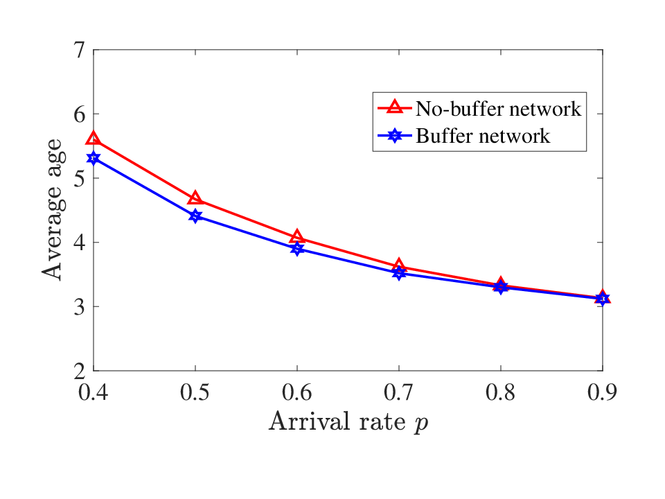
To study the effect of the buffers, we consider the truncated MDP with the boundary and generate arrivals with . After averaging the age over 100,000 slots, we obtain the average age in Fig. 9 for various , where the red curve with the triangle markers indicates the no-buffer networks (by employing Alg. 1) and the blue curve with the star markers indicates the network with the buffers.
In this setting, we see mild improvement of the average age by exploiting the buffers. The buffers reduce the average age by only around when , and even lower when is higher. Let us discuss the following three cases when both users have arrivals in some slot:
- •
When both and are high: That means the user who is not updated currently has a new arrival in the next slot with a high probability; as such, the old packet in the buffer seems not that effective.
- •
When both and are low: Then, the possibility of the two arrivals in the same slot is very low. Hence, this would be a trivial case.
- •
When one of and are high and the other is low: In this case, the BS will give the user with the lower arrival rate a higher update priority, as a packet for the other user will arrive shortly.
According to the above discussions, we observe that the buffers might not be that effective as expected. The no-buffer network is not only simple for practical implementation but also works well.
VII Concluding remarks
In this paper, we treated a wireless broadcast network, where many users are interested in different information that should be delivered by a base-station. We studied the age of information by designing and analyzing four scheduling algorithms, i.e., the structural MDP scheduling algorithm, the index scheduling algorithm, the MPD-based online scheduling algorithm, and the index-based online scheduling algorithm. We not only theoretically investigated the optimality of the proposed algorithms, but also validate their performance via the computer simulations. It turns out that the low-complexity index scheduling algorithm and both online scheduling algorithms almost achieve the minimum average age.
Some possible future works are discussed as follows. We focused on the no-buffer network in this paper. It is an issue to study provable effectiveness of the buffers and to characterize the regime under which the no-buffer network works with marginal performance loss. Moreover, it is interesting to investigate structural results like ours for simplifying the calculation of the Whittle index for networks with buffers. Finally, the paper treated a single-hop network only. It is interesting to extend our results to multi-hop networks.
Acknowledgments
The work of Yu-Pin Hsu is supported by Ministry of Science and Technology, Taiwan (Project No. 107-2221-E-305-007-MY3).
References
- [1] Y.-P. Hsu, E. Modiano, and L. Duan, “Age of Information: Design and Analysis of Optimal Scheduling Algorithms,” Proc. of IEEE ISIT, pp. 561–565, 2017.
- [2] Y.-P. Hsu, “Age of Information: Whittle Index for Scheduling Stochastic Arrivals,” Proc. of IEEE ISIT, 2017.
- [3] S. Kaul, R. D. Yates, and M. Gruteser, “Real-Time Status: How Often Should One Update?” Proc of IEEE INFOCOM, pp. 2731–2735, 2012.
- [4] D. P. Bertsekas, Dynamic Programming and Optimal Control Vol. I and II. Athena Scientific, 2012.
- [5] J. Cho and H. Garcia-Molina, “Synchronizing a Database to Improve Freshness,” Proc. of ACM SIGMOD, vol. 29, no. 2, pp. 117–128, 2000.
- [6] C. Kam, S. Kompella, G. D. Nguyen, and A. Ephremides, “Effect of Message Transmission Path Diversity on Status Age,” IEEE Trans. Inf. Theory, vol. 62, no. 3, pp. 1360–1374, 2016.
- [7] Y. Sun, E. Uysal-Biyikoglu, R. D. Yates, C. E. Koksal, and N. B. Shroff, “Update or Wait: How to Keep Your Data Fresh,” Proc. of IEEE INFOCOM, pp. 1–9, 2016.
- [8] R. D. Yates, “Lazy is Timely: Status Updates by an Energy Harvesting Source,” Proc. of IEEE ISIT, pp. 3008–3012, 2015.
- [9] B. T. Bacinoglu, E. T. Ceran, and E. Uysal-Biyikoglu, “Age of Information under Energy Replenishment Constraints,” Proc. of ITA, pp. 25–31, 2015.
- [10] M. Costa, M. Codreanu, and A. Ephremides, “On the Age of Information in Status Update Systems with Packet Management,” IEEE Trans. Inf. Theory, vol. 62, no. 4, pp. 1897–1910, 2016.
- [11] Q. He, D. Yuan, and A. Ephremides, “Optimal Link Scheduling for Age Minimization in Wireless Systems,” accepted to IEEE Trans. Inf. Theory, 2017.
- [12] C. Joo and A. Eryilmaz, “Wireless Scheduling for Information Freshness and Synchrony: Drift-based Design and Heavy-Traffic Analysis,” Proc. of IEEE WIOPT, pp. 1–8, 2017.
- [13] Y. Sun, E. Uysal-Biyikoglu, and S. Kompella, “Age-Optimal Updates of Multiple Information Flows,” Proc. of IEEE INFOCOM Workshops-AoI Workshop, 2018.
- [14] I. Kadota, E. Uysal-Biyikoglu, R. Singh, and E. Modiano, “Minimizing Age of Information in Broadcast Wireless Networks,” Proc. of Allerton, 2016.
- [15] R. D. Yates, P. Ciblat, A. Yener, and M. Wigger, “Age-Optimal Constrained Cache Updating,” Proc. of IEEE ISIT, pp. 141–145, 2017.
- [16] M. L. Puterman, Markov Decision Processes: Discrete Stochastic Dynamic Programming. The MIT Press, 1994.
- [17] R. Cavazos-Cadena, “A Counterexample on the Optimality Equation in Markov Decision Chains with the Average Cost Criterion,” Systems & control letters, vol. 16, no. 5, pp. 387–392, 1991.
- [18] L. I. Sennott, “Average Cost Optimal Stationary Policies in Infinite State Markov Decision Processes with Unbounded Costs,” Operations Research, vol. 37, pp. 626–633, 1989.
- [19] ——, Stochastic Dynamic Programming and the Control of Queueing Systems. John Wiley & Sons, 1998.
- [20] J. Gittins, K. Glazebrook, and R. Weber, Multi-Armed Bandit Allocation Indices. John Wiley & Sons, 2011.
- [21] M. Larranaga, U. Ayesta, and I. M. Verloop, “Stochastic and Fluid Index Policies for Resource Allocation Problems,” Proc. of IEEE INFOCOM, pp. 1230–1238, 2015.
- [22] I. Kadota, A. Sinha, and E. Modiano, “Optimizing Age of Information in Wireless Networks with Throughput Constraints,” to be appeared in Proc. of IEEE INFOCOM, 2018.
- [23] W. B. Powell, Approximate Dynamic Programming: Solving the Curses of Dimensionality. John Wiley & Sons, 2011.
- [24] N. Salodkar, A. Bhorkar, A. Karandikar, and V. S. Borkar, “An On-Line Learning Algorithm for Energy Efficient Delay Constrained Scheduling over a Fading Channel,” IEEE J. Sel. Areas Commun., vol. 26, no. 4, pp. 732–742, 2008.
- [25] P. Whittle, “Restless Bandits: Activity Allocation in a Changing World,” Journal of applied probability, pp. 287–298, 1988.
- [26] V. S. Borkar, Stochastic Approximation: A Dynamical Systems Viewpoint. Cambridge University Press, 2008.
- [27] V. S. Borkar and S. P. Meyn, “The ODE Method for Convergence of Stochastic Approximation and Reinforcement Learning,” SIAM Journal on Control and Optimization, vol. 38, no. 2, pp. 447–469, 2000.
- [28] J. Abounadi, D. Bertsekas, and V. Borkar, “Learning Algorithms for Markov Decision Processes with Average Cost,” SIAM Journal on Control and Optimization, vol. 40, no. 3, pp. 681–698, 2001.
- [29] L. Georgiadis, M. J. Neely, and L. Tassiulas, Resource Allocation and Cross-Layer Control in Wireless Networks. Now Publishers Inc, 2006.
- [30] L. I. Sennott, “On Computing Average Cost Optimal Policies with Application to Routing to Parallel Queues,” Mathematical Methods of Operations Research, vol. 45, pp. 45–62, 1997.
- [31] R. G. Gallager, Discrete Stochastic Processes. Springer Science & Business Media, 2012, vol. 321.
Appendix A Proof of Proposition 4
According to [18], it suffices to show that for every initial state and discount factor . Let be the deterministic stationary policy of the MDP that chooses for all . Note that, for initial state , we have
By definition of the optimality, we conclude since .
Appendix B Proof of Proposition 5
The proof is based on induction on of the value iteration in Eq (4). The result clearly holds for . Suppose that is non-decreasing in . First, note that the immediate cost is a non-decreasing function in . Second, is also a non-decreasing function in according to the induction hypothesis. Since the minimum operator (in Eq. (4)) holds the non-decreasing property, we conclude that is a non-decreasing function as well.
Appendix C Proof of Lemma 6
We divide state space into two disjoint sets and , where the age vectors in the set belongs to . Then, set is a transient set for any scheduling algorithm that will update each user for at lease once. We consider two cases as follow.
First, we focus on the MDP with the restricted state space , and show the lemma holds. According to [18], we need to verify that the following two conditions are satisfied.
- 1.
There exists a deterministic stationary policy of the MDP such that the resulting discrete-time Markov chain (DTMC) by the policy is irreducible, aperiodic, and the average cost is finite: We consider the deterministic stationary policy as the one that updates a user with an arrival and the largest age. It is obvious that the resulting DTMC is irreducible and aperiodic. Next, we transform the age of information into an age-queueing network in Fig. 10 consisting of age-queues , age-packet arrivals to each queue, and a server. In each slot an age-packet arrives at the system, since the age increases by one for each slot. In each slot a channel associated with queue is ON with probability . For each slot the server can serve a queue with an infinite number of age-packets if its channel is ON. Then, the long-run average total age-queue size is the average cost. Note that the arrival rate is interior of the capacity region [29] of the age-queueing network. Moreover, the policy is the maximum weight scheduling algorithm [29] that is shown to be throughput-optimal; as such, the average age-queue size is finite. Thus, the average cost is finite as well.

Fig. 10: Age-queueing network. - 2.
There exists a nonnegative such that the relative cost function for all and : Let be the expected cost of the first passage from state to state under policy . Then, using the deterministic stationary policy in the first condition, we have (see [18, Proposition 4]) and (see [18, proof of Proposition 5]). Moreover, as is a non-decreasing function in (see our Proposition 5), only state with for all can probably result in a lower value of than . We hence can choose .
Thus, according to [18], there exists a deterministic stationary policy that is -optimal and minimum average cost is the constant , independent of the initial state.
Second, we note that, if the initial state belongs to , then a -optimal policy will update each user for at least once (e.g, using the above deterministic scheduling algorithm ); otherwise, the average cost is infinite. In other words, state will enter in finite time, and always stay in the set onwards. Thus, the average cost until the state enters approaches zero as slots go to infinity, and the minimum average cost is still the constant as in the first case. Moreover, there exists a deterministic stationary policy that is -optimal, e.g., following the deterministic stationary policy before entering and then following the -optimal deterministic stationary policy in the first case.
Appendix D Proof of Theorem 9
Let and be the minimum expected total -discounted cost and the relative cost function for the MDP , respectively. According to [30], we need to prove the following two conditions are satisfied.
- 1.
There exists a nonnegative , a nonnegative finite function on such that for all , where and : We consider a randomized stationary algorithm that updates each user (with packet arrival) with equal probability for each slot. Similar to Appendix C, let and be the expected cost from state to the reference state by applying the algorithm to and , respectively. Then, and similar to Appendix C. In the following, we will show that and then we can choose the function .
To that end, we first express as
for some (or no) excess probabilities [30] on some state , depending on next state . Since the scheduling algorithm is independent of the age, given arrival vector we have for age vector . Then, we obtain
(13) Using the above inequality, we then conclude because
On the other hand, we can choose , since (see Appendix C) and similar to above.
- 2.
The value is bounded by , i.e., : We claim that for all , and then the condition holds as
Remark 23.
Here, we want to emphasize that we have chosen . If not, the state space of the MDP would have to include more transient states such that all ages are no more than , e.g., the age vector of . These additional states are not reachable from state . Thus, we cannot choose the as in the proof, since is infinite if the age vector in state is .
Appendix E Proof of Theorem 10
According to [16, Theorem 8.6.6], the RVIA in Eq. (5) converges to the optimal solution in finite iterations if the truncated MDP is unichain, i.e., the Markov chain corresponding to every deterministic stationary policy consists of a single recurrent class plus a possibly empty set of transient states. Note that for every truncated MDP, there is only one recurrent class by [31], since the state is reachable (e.g., there is no arrival in the next slots) from all other states (where remember that is the boundary of the truncated MDP). Hence, the truncated MDPs are unichain and the theorem follows immediately.
Appendix F Proof of Theorem 12
Given initial state , we define the expected total -discounted cost under policy by
Let be the minimum expected total -discounted cost. A policy that minimizes is called -optimal policy. Again, we check the two conditions in Appendix C.
- 1.
Let be the deterministic stationary policy of always choosing action for each slot if there is an arrival. It is obvious that the resulting DTMC by the policy is irreducible and aperiodic. To calculate the average cost, we note that age by the policy is also a DTMC in Fig. 11. The steady-state distribution of the DTMC is
Hence, the average age is
On the other hand, the average updating cost is as the arrival probability is . Hence, the average cost under the policy is the average age (i.e., ) plus the average updating cost (i.e., ), which is finite.

Fig. 11: The age under the policy forms a DTMC. - 2.
Similar to Proposition 5, we can show that is a non-decreasing function in age for a given arrival indicator ; moreover, is a non-increasing function in for a given age . Thus, we can choose .
By verifying the two conditions, the theorem immediately follows from [18].
Appendix G Proof of Lemma 18
Since is the updating cost to make both actions for state equally desirable and we break a tie in favor of idling, the optimal threshold is if the cost is , for all . We claim that the optimal threshold monotonically increases with cost , and then the theorem follows.
To verify the claim, we can focus on the discounted cost case according to the proof of Theorem 8. Suppose that an -optimal action, associated with a cost , for state is to idle, i.e.,
Then, an -optimal action, associated with a cost , for state is to idle as well since
Then, the monotonicity is established.
Appendix H Proof of Lemma 21
Similar to the proof of Theorem 8, we can focus on the discounted cost case. Without loss of generality, we assume that age .
Let be the zero vector except for the -the entry being replaced by . By the symmetry of the users, swap of the initial ages of any two users results in the same expected total -discounted cost, i.e.,
for all . Similar to the proof of Theorem 8, here we focus on the case when and . The result follows from the non-decreasing function of and for all :