First results from the LIFE project: discovery of two magnetic hot evolved starsThanks: Based on observations obtained at the Canada-France-Hawaii Telescope (CFHT) operated by the National Research Council of Canada, the Institut National des Sciences de l’Univers of the CNRS of France, and the University of Hawaii.
Abstract
We present the initial results of the Large Impact of magnetic Fields on the
Evolution of hot stars (LIFE) project. The focus of this project is the search for
magnetic fields in evolved OBA giants and supergiants with
visual magnitudes between 4 and 8, with the aim to investigate how
the magnetic fields observed in upper main sequence (MS) stars evolve from the MS until the late post-MS stages. In this paper, we present spectropolarimetric
observations of 15 stars observed using the ESPaDOnS instrument of the CFHT.
For each star, we have determined the fundamental parameters and
have used stellar evolution models to calculate their mass, age and radius.
Using the LSD technique, we have produced averaged line profiles for each star. From these profiles,
we have measured
the longitudinal magnetic field strength and have calculated the detection probability.
We report the detection of magnetic fields in two stars of our sample:
a weak field of G is detected in the post-MS A5 star 19 Aur and a stronger field of
G is detected in the MS/post-MS B8/9 star HR 3042.
Keywords:
stars: magnetic fields – stars: early-type – stars: supergiants – stars:evolution – techniques: spectroscopic – techniques: polarimetric
1 Introduction
The last decade has seen a remarkable increase in our knowledge of the properties of magnetic fields in main sequence (MS) OB type stars. As a result of a number of surveys (Fossati et al., 2015b; Fossati et al., 2015a; Wade et al., 2016; Grunhut et al., 2017, e.g.,), convincing evidence indicates that 10% of MS OB stars are magnetic. This is consistent with the findings for MS A stars (Power et al., 2008; Aurière et al., 2007). MS OB stars host roughly dipolar, often oblique fossil magnetic fields (Neiner et al., 2015; Grunhut & Neiner, 2015). There is currently no known mechanism to generate and sustain an efficient dynamo field in a radiative envelope, which would affect the global fossil field during the MS phase of OB type stars (Zahn et al., 2007; Rüdiger et al., 2012; Neiner et al., 2015). The observed fossil fields likely formed in the pre-MS phases: during its formation the star could ensnare the weak field present in the interstellar medium (ISM) and dynamo fields generated during pre-MS stages can enhance this seed field (Mestel, 1999; Alecian et al., 2008). The field then relaxes to a stable configuration, which is mainly dipolar at the surface (Braithwaite & Spruit, 2004; Duez & Mathis, 2010).
Since no dynamo field is observed in MS OB stars, there is nothing to replenish the field over time. It has been shown by Bagnulo et al. (2006); Landstreet et al. (2007); Landstreet et al. (2008) and Fossati et al. (2016), that the magnetic fields at the surface of stars decrease with stellar age on the MS. This decrease in strength likely occurs in part as a result of flux conservation in response to the increase in stellar radius, possibly altered by Ohmic decay or other currently unknown effects.
Furthermore, it is likely that the stellar magnetic field has a strong influence on the evolution of the host star (Moss, 1984; Langer, 2012; Maeder & Meynet, 2014; Keszthelyi et al., 2017; Georgy et al., 2017). The effects of the field can be separated into those operating at the surface of the star and those in the interior. Theoretical models predict that interactions between the magnetic field and the stellar wind can reduce the surface mass-loss and stellar rotation rate (ud-Doula & Owocki, 2002; ud-Doula et al., 2008; ud-Doula et al., 2009; Meynet et al., 2011; Bard & Townsend, 2016). Indeed, studies of massive stars show that the stellar wind can become trapped in a magnetosphere rigidly coupled to the star’s magnetic field (Landstreet & Borra, 1978; Oksala et al., 2015). Conservation of angular momentum then leads to a decrease in the rotation rate of the star (Townsend et al., 2010; Mikulášek et al., 2007, e.g.,). In the stellar interior, the magnetic field has the potential to affect the mixing and diffusion of chemical elements, the internal rotational profile and angular momentum (Mestel, 1999; Mathis & Zahn, 2005; Briquet et al., 2012; Sundqvist et al., 2013; Maeder & Meynet, 2014; Stift & Alecian, 2016).
In general, however, magnetic fields have not been taken into account in evolutionary models, except for Taylor-Spruit dynamo fields (Maeder & Meynet, 2003; Heger et al., 2005, e.g.,), which are themselves inconsistent with those observed in MS OBA type stars. In particular, the observed fields are not correlated with rotation as would be expected for an dynamo like that proposed by Spruit (2002). It is therefore important to study these stars in detail to provide observational constraints to stellar evolution models. However, the structural changes which occur in a star during the MS are, in general, not sufficient to allow us to understand how magnetic fields change as stars evolve and how stars respond to the presence of a magnetic field.
One potential pathway towards exploring the evolution of magnetic fields in massive stars lies in the study of evolved OBA stars. We already have convincing evidence that 10% of MS OB stars have magnetic fields (Grunhut & Neiner, 2015; Fossati et al., 2015b; Grunhut et al., 2017), and the same appears to be true for PMS stars (Alecian et al., 2013). It is reasonable to suspect that the same may well be true for evolved descendants. These stars not only provide the possibility to study the evolution of magnetic fields over a longer evolutionary time-frame, but also to investigate the evolution of the magnetic field in response to the significant changes in stellar structure occurring during the star’s transition through the post-MS.
As the star moves through the post-MS, its radius vastly increases (Ekström et al., 2012; Georgy et al., 2013; Sanyal et al., 2015, e.g.,). Initially, the fossil field structure should remain unchanged, since the radiative envelope still exists and there is no mechanism to allow for the formation of a dynamo. However, as the star continues to evolve, convective zones form in the upper regions of the stellar envelope (Neiner et al., 2017, e.g.,). These regions have the potential to generate dynamo magnetic fields. These new dynamo fields might have a significant impact on the fossil field already present in the star (Featherstone et al., 2009; Aurière et al., 2008). Indeed the studies of FGK type giants and supergiants show magnetic fields powered by dynamos (Grunhut et al., 2010; Aurière et al., 2015, e.g.,). These stars are the evolutionary descendants of OBA type MS stars and so it is possible that a star originally with a fossil magnetic field on the MS experiences a period with both a fossil field and dynamo field, and finally evolves to a state in which only the dynamo field signature can be observed. In fact, the intermediate mass red giant star EK Eri shows tantalising evidence that it hosts both a dynamo field and the remnant of an Ap fossil field (Aurière et al., 2011).
Until very recently, no post-MS magnetic OBA stars had been unambiguously identified, despite high-precision studies having been conducted (Verdugo et al., 2005; Shultz et al., 2014, e.g.,). The O9.5 supergiant Ori A was found to have a magnetic field (Bouret et al., 2008; Blazère et al., 2015), however, this star was shown to likely be still on the MS (Fossati et al., 2015a), despite its supergiant classification. A magnetic field was also detected in the B1.5 star CMa by Fossati et al. (2015a); Neiner et al. (2017) showed however, that this star is also located at the end of its MS phase. As part of the BRIght Target Explorer spectropolarimetric survey (Neiner et al., 2016, BRITEpol;), Neiner et al. (2017) identified two magnetic A7 supergiants: Car and HR 3890. Luminosity measurements and the fundamental parameters associated with these stars indicate that they are well into the post-MS phase of evolution. The detected longitudinal magnetic field strengths were found to be roughly 10 and 1 G for Car and HR 3890, respectively. As a result, we infer that any survey would need to be able to detect magnetic fields to a precision of better than 1 G, in order to determine the incidence rate of magnetic fields in evolved OBA type stars.
To this end, we have started the Large Impact of magnetic Fields on the Evolution of hot stars (LIFE) project. We are observing the circularly polarised spectrum and measuring the longitudinal magnetic field strength () of OBA type stars between V = 4 mag and V = 8 mag with luminosity classes I-III. In this paper, we present the analysis of the first 15 stars observed for this study. Section 2 gives details of the LIFE project, the observations and data reduction. The fundamental parameters we infer for each star are given in Section 3 along with the evolutionary status of each star. In Section 4 we give details of the magnetic field detections and finally in Sections 5 and 6 we discuss our findings and conclude the paper.
2 The LIFE project
| Star | HD No. | Visual | Date | Exp. Seq. | mid-HJD | Average | LSD | LSD | Lines |
|---|---|---|---|---|---|---|---|---|---|
| Magnitude | (UT) | (s) | -2450000 | S/N | S/N | S/N | in LSD | ||
| 13 Mon | 46300 | 4.47 | Feb 18, 2016 | 2x4x138 | 7437.8113 | 758 | 3536 | 13603 | 1394 |
| 15 Sgr | 167264 | 5.29 | May 14, 2016 | 2x4x344 | 7524.1189 | 911 | 1610 | 6816 | 69 |
| May 17, 2016 | 4x4x344 | 7526.9869 | 863 | 2229 | 9234 | 69 | |||
| May 18, 2016 | 2x4x344 | 7528.0034 | 921 | 1552 | 6885 | 69 | |||
| 19 Aur | 34578 | 5.05 | Sep 18, 2016 | 5x4x254 | 7651.0154 | 1034 | 4031 | 55620 | 4298 |
| Oct 20, 2016 | 5x4x254 | 7683.0600 | 1067 | 3808 | 56872 | 4297 | |||
| 24 CMa | 53138 | 3.02 | Feb 28, 2016 | 23x4x40 | 7447.8037 | 983 | 4466 | 48600 | 538 |
| Leo | 87737 | 3.48 | Feb 21, 2016 | 5x4x50 | 7440.8394 | 535 | 3735 | 17673 | 1781 |
| CMa | 53244 | 4.11 | Dec 20, 2016 | 12x4x143 | 7744.0163 | 1111 | 14049 | 60259 | 1293 |
| HD 10362 | 10362 | 6.33 | Sep 17, 2016 | 1x4x991 | 7649.9784 | 1187 | 2270 | 13094 | 476 |
| Sep 19, 2016 | 1x4x991 | 7651.8850 | 1238 | 2326 | 13619 | 476 | |||
| HD 42035 | 42035 | 6.55 | Sep 21, 2016 | 1x4x1313 | 7654.0594 | 1316 | 4327 | 22097 | 2649 |
| HD 186660 | 186660 | 6.47 | Oct 13, 2016 | 1x4x1122 | 7675.7705 | 1112 | 1850 | 7975 | 327 |
| HD 188209 | 188209 | 5.6 | Jun 19, 2016 | 8x4x443 | 7560.0473 | 1017 | 1669 | 19678 | 227 |
| HD 209419 | 209419 | 5.79 | Oct 12, 2016 | 1x4x666 | 7674.8808 | 1035 | 4305 | 13777 | 600 |
| HIP 38584 | 64827 | 6.85 | Mar 13, 2017 | 1x4x1049 | 7826.8619 | 728 | 4861 | 13323 | 864 |
| HR 3042 | 63655 | 6.23 | Dec 14, 2016 | 3x4x981 | 7738.0787 | 1233 | 5628 | 21271 | 201 |
| PT Pup | 61068 | 5.69 | Dec 20, 2016 | 1x4x559 | 7743.9491 | 1105 | 1330 | 13114 | 304 |
| V399 Lac | 210221 | 6.17 | Jun 14, 2016 | 4x4x604 | 7555.0612 | 846 | 2447 | 29738 | 1631 |
Through the LIFE project, we aim to measure the distribution of magnetic field strengths in evolved stars and compare our findings with the results for MS OB stars. Any detected field will be fully characterised and the results will be compared with those of MS stars to determine how the magnetic fields of stars change as stars evolve. From this project we aim to provide important observational constraints on theories of how magnetic fields and stellar evolution affect and interact with each other.
Choosing the appropriate exposure time for each star is critically important to give us the best possible chance of detecting magnetic fields for our sample of stars. As a result of the MiMeS (Wade et al., 2016), BinaMIcS (Alecian et al., 2015) and BRITEpol (Neiner et al., 2016) surveys we have an accurate exposure time relationship (Wade et al., 2016) which predicts the spectral signal-to-noise ratio (S/N) required to detect magnetic fields to a certain precision, given the spectral type and rotational velocity of a star11 1 To plan the observations, we considered the rotational velocities found through Vizier. If none were present for a given star, we assumed a value of 50 km s-1.. It is then straightforward to obtain the necessary exposure time required for each star.
However, we cannot know a priori the current dipole magnetic field strength () of the stars; therefore it is necessary to adopt a plausible distribution for the magnetic field. We calculate this by comparing the current radius of the star () with its radius at the zero-age main sequence () assuming that the magnetic flux is conserved. We calculate the expected current surface magnetic field strength to be
| (1) |
where is the magnetic field strength at the ZAMS. The choice of is important, because we are limited by total exposure time. For this work, we assume that kG or if this would lead to an exposure time longer than one night, then kG. These values correspond to 95% and 85% completeness of the observed distribution of magnetic field strengths in MS stars respectively (Shultz, 2016, and Shultz et al. in prep.). The predicted for our sample is between 10 and 100 which means we expect to detect dipole fields of between 7 G and 140 G.
We do not, however, measure . Instead, we measure the mean longitudinal field which is a function of the inclination angle () of the star and the obliquity angle () between the rotation axis and the magnetic axis (Preston, 1967). For our stars, and were not available prior to the observations and so we use the equations from Preston (1967) to estimate that conservatively is 3 times weaker than . This lower value is factored into our calculations of the total required exposure time for each star.
2.1 Observations
The LIFE observations we present in this paper were taken using the ESPaDOnS (an Echelle SpectroPolarimetric Device for the Observation of Stars) instrument at the Canada France Hawaii Telescope (CFHT) and are summarised in Table 1. We observe over a wavelength range from about 3700 Å to 10500 Å with a resolving power of 68000. Each spectrum is spread over 40 echelle orders. The observations are corrected for the bias and flat-field, and a ThAr spectrum is used to calibrate the wavelengths to the pixel values. The data were reduced using Libre-Esprit (Donati et al., 1999) and Upena, a software pipeline available at the CFHT.
The data were taken in circular spectropolarimetric mode, measuring Stokes and . Each observation sequence consists of four sub-exposures, taken with different orientations of the Fresnel rhombs. The observations were constructively combined to form Stokes and destructively combined to form the null spectra, (Donati et al., 1997), using the ratio method (Bagnulo et al., 2009). Adding all four observations together provides Stokes . If the total exposure time calculated in Section 2 was expected to saturate the detector, we took a number of consecutive sequences of the four sub-exposures which add up to the total required exposure time. These observations are then co-added after we have produced each least-squared deconvolution (LSD) profile (see Section 2.3).
2.2 Normalisation of stellar spectra
We used a semi-automatic Python program (Martin et al., 2017, and Appendix A) to determine the continuum shape of the Stokes spectrum, fitting each ESPaDOnS order individually. The Python program allows the user to fit a third-order spline to the continuum. This is achieved by initially fitting a third-order spline to the reduced unnormalised spectrum. Points from the spectrum are then iteratively -clipped about the spline, until only continuum points remain. For the majority of spectra the -clipping is asymmetric with more points clipped below than above the fit (e.g., = 3 and = 1 ). This is because, to obtain a good continuum fit, all spectral lines must be removed and for the stars in this sample we mainly observe absorption lines. However, each parameter which determines the final continuum fit can be changed interactively including the number of iterations, the number of knots defining the cubic spline, and the -clipping bounds. Finally, we take the best continuum model calculated for each star and use it to normalise the Stokes and and spectra.
2.3 Least Squares Deconvolution
During this project we are searching for very weak magnetic fields, between 1 and 100 G. This leads to Stokes signatures with very low amplitudes. To detect such tiny signatures, we use the LSD technique (Donati et al., 1997) and combine multiple consecutive observations to increase the S/N of our data. We calculate mean LSD Stokes , Stokes and profiles and co-add consecutive observations to produce the LSD line profiles which we use to measure the magnetic field of our observed stars. Since we aim to reduce all sources of noise we must take care when producing the line mask. The line mask is used to determine which lines to include in the LSD profile and to provide the LSD routine with the parameters of each line including their wavelength, relative depth, and Landé factor. To start, we extract a stellar line list from the VALD3 database (Piskunov et al., 1995; Kupka et al., 1999). This line list is calculated with the and which we determine for each of our stars (see Section 3.1). However, it will contain lines which are not present in the stellar spectrum and other lines which will add noise to the LSD profile. Therefore, we comb through each list, first removing lines with a depth smaller than 0.01 (relative to a continuum level of 1), and those which we do not see in our observed spectra. We remove hydrogen lines, because their shape is different from metal lines, and we remove any lines which blend with either H, interstellar, or strong telluric lines. Finally, we adjust the depth of each remaining line in the line mask so that it is consistent with the observed spectrum, in the manner described by Grunhut et al. (2017).
3 Stellar properties
| Star | Spectral | ||||||||
| Type | (K) | (cgs) | (km s-1) | (km s-1) | |||||
| 13 Mon | A1Ib1 | 10250 | 300 | 2.2 | 0.2 | 13.4 | 0.1 | 13.21 | 0.02 |
| 15 Sgr | O9.7Iab2 | 30000 | 1000 | 3.5 | 0.2 | 58 | 1 | 19.8 | 0.1 |
| 19 Aur | A5Ib-II3 | 8500 | 200 | 2.0 | 0.2 | 8.8 | 0.1 | -3.15 | 0.01 |
| 24 CMa | B4Ia1 | 17000 | 400 | 2.1 | 0.2 | 39.2 | 0.4 | 48.08 | 0.07 |
| Leo | A0Ib1 | 9750 | 300 | 2.0 | 0.2 | 13.9 | 0.1 | 2.82 | 0.02 |
| CMa | B6III1 | 13600 | 300 | 3.4 | 0.2 | 37 | 1 | 31.1 | 0.2 |
| HD 10362 | B7III4 | 14300 | 300 | 3.3 | 0.2 | 30.1 | 0.7 | -6.0 | 0.1 |
| HD 42035 | B9V5 | 10500 | 200 | 3.5 | 0.2 | 4 | 1 | 2.3 | 0.02 |
| HD 186660 | B2III/IV6 | 16900 | 300 | 3.6 | 0.2 | 11.4 | 0.1 | -16.65 | 0.02 |
| HD 188209 | O9.5Iab7 | 30000 | 1000 | 3.1 | 0.2 | 84 | 1 | -18.78 | 0.08 |
| HD 209419 | B5V8 | 14100 | 300 | 3.5 | 0.2 | 14.5 | 0.3 | -16.23 | 0.05 |
| HIP 38584 | B8II9 | 12600 | 300 | 3.0 | 0.2 | 28.4 | 0.6 | 30.0 | 0.1 |
| HR 3042 | B8/9II10 | 14150 | 300 | 3.5 | 0.2 | 60 | 1 | -4.5 | 0.2 |
| PT Pup | B1V11 | 26300 | 500 | 4.1 | 0.2 | 16.9 | 0.1 | 37.83 | 0.02 |
| V399 Lac | A3Ib3 | 8500 | 200 | 1.5 | 0.2 | 11.8 | 0.1 | -25.30 | 0.01 |
| Note: taken from 1Zorec et al. (2009), 2Sota et al. (2014), 3Abt & Morrell (1995), | |||||||||
| 4Jensen (1981), 5Molnar (1972), 6Houk & Swift (1999), 7Sota et al. (2011), | |||||||||
| 8Gkouvelis et al. (2016), 9Houk (1978), 10Houk & Smith-Moore (1988), 11Nieva (2013). | |||||||||
3.1 Fundamental parameters
For each star we calculated the effective temperature () and surface gravity () using the uvbybeta code (Napiwotzki et al., 1993). We also used grids of synthetic spectra to visually check that the values accurately reproduce primarily the H, H, H and H lines, but also regions of metal lines. Examples of the fit between the synthetic and observed spectrum for H are shown in Fig. 1. The grids of synthetic spectra we used were calculated by Bohlin et al. (2017, using atlas9 model atmospheres), Martin et al. (2017, using atlas9 model atmospheres) and Lanz & Hubeny (2007, using tlusty model atmospheres). In the case of atlas9 model atmospheres (Kurucz, 1993b), the synthetic spectra are calculated assuming plane parallel geometry, local thermodynamic equilibrium (LTE) and opacity distribution functions (ODFs) for solar abundances (Kurucz, 1993a). The synthetic spectra were computed with cossam_simple (Martin et al., 2017) and synthe (Kurucz & Avrett, 1981; Bohlin et al., 2017). For the tlusty model atmospheres the synthetic spectra are calculated assuming non-local thermodynamic equilibrium, plane-parallel geometry and hydrostatic equilibrium using synspec (Hubeny & Lanz, 2011). Where necessary we calculated additional synthetic spectra using atlas9 model atmospheres and synspec.
To calculate the projected rotational velocity () and the radial velocity () for each star, we first fit a Gaussian to the LSD profile. The mean value of this Gaussian is adopted as the of the star. We then subtract from the velocity of each pixel such that the line center of the LSD profile is shifted to 0 kms-1. We apply a Fast Fourier transform (FFT) to the profile. Following Gray (2005) and Glazunova et al. (2008), the first minimum of the transform is related to the stellar value by the limb darkening coefficient. The limb darkening value varies as a function of stellar and ; for each of our stars we use limb darkening values from Claret & Bloemen (2011) which are consistent with our calculated and values.
We calculate the minimum error on () following Seager et al. (2010) as
| (2) |
where is the full width half maximum of the LSD profile and is the maximum intensity value of the inverse of the LSD profile. We calculate the error on () following Díaz et al. (2011) as
| (3) |
where rms is the root mean square of the LSD profile.
To check the consistency of the calculated
and values, we compare the observed spectrum with a
synthetic spectrum calculated using our derived fundamental parameters and we find that they agree well.
| Star | Parallax | Bolometric | MZAMS | RZAMS | M | R | Age | Turn-off | Exp. Field | ||||||
|---|---|---|---|---|---|---|---|---|---|---|---|---|---|---|---|
| (mas) | correction | () | () | (M⊙) | () | (R⊙) | (M⊙) | (R⊙) | (Myr) | Age (Myr) | (G) | ||||
| 13 Mon | 0.8 | 0.5 | -6.1 | -0.30 | 4.4 | 3.2 | 0.1 | 15.0 | 0.60 | 4.7 | 14.7 | 91.9 | 13.8 | 13.6 | 1 |
| 8.0 | 0.00 | 3.2 | 8.0 | 23.8 | 33.3 | 32.9 | 11 | ||||||||
| 15 Sgr | 0.1 | 0.5 | -10.0 10.0 | -2.89 | 7 4 | 3.79 | 0.09 | 32.0 | 0.00 | 6.9 | 30.3 | 18.1 | 4.8 | 5.2 | 92 |
| 23.0 | 0.00 | 5.7 | 22.5 | 12.3 | 5.9 | 6.8 | 140 | ||||||||
| 19 Aur | 1.6 | 0.3 | -4.4 | -0.00 | 3.7 0.2 | 3.1 | 0.1 | 10.0 | 0.00 | 3.6 | 9.7 | 59.3 | 23.8 | 20.9 | 2 |
| 7.0 | 0.60 | 3.1 | 6.9 | 36.8 | 56.7 | 51.0 | 4 | ||||||||
| 24 CMa | 1.2 | 0.4 | -6.7 | -1.53 | 5.2 | 4.2 | 0.1 | 40.0 | 0.00 | 7.8 | 16.1 | 71.6 | 4.6 | 4.5 | 7 |
| 15.0 | 0.59 | 4.7 | 14.7 | 29.4 | 13.6 | 13.5 | 16 | ||||||||
| Leo | 2.6 | 0.2 | -4.5 0.1 | -0.20 | 3.77 | 3.3 | 0.2 | 12.0 | 0.98 | 4.8 | 11.9 | 66.6 | 20.3 | 19.2 | 3 |
| 8.0 | 0.00 | 3.2 | 8.0 | 25.9 | 33.3 | 32.9 | 9 | ||||||||
| CMa | 7.4 | 0.2 | -1.49 0.06 | -1.00 | 2.88 | 2.5 | 0.1 | 7.0 | 0.00 | 2.9 | 7.0 | 11.5 | 42.3 | 41.8 | 41 |
| 5.0 | 0.98 | 2.9 | 5.0 | 5.5 | 98.9 | 113.6 | 170 | ||||||||
| HD 10362 | 2.4 | 0.5* | -2.2 | -1.12 | 3.2 0.2 | 2.7 | 0.1 | 7.0 | 0.11 | 3.0 | 7.0 | 10.7 | 45.2 | 44.7 | 48 |
| 5.0 | 0.33 | 2.5 | 5.0 | 5.3 | 97.8 | 104.5 | 140 | ||||||||
| HD 186660 | 2.1 | 0.5* | -2.7 | -1.52 | 3.6 0.2 | 2.70 | 0.09 | 8.0 | 0.00 | 3.2 | 8.0 | 9.4 | 33.2 | 32.9 | 72 |
| 7.0 | 0.97 | 3.5 | 7.0 | 6.5 | 46.5 | 52.8 | 180 | ||||||||
| HD 188209 | 0.9 | 0.2 | -5.4 | -2.89 | 5.2 0.2 | 4.19 | 0.09 | 84.9 | 0.00 | 12.2 | 70.0 | 40.9 | 2.5 | 3.0 | 56 |
| 20.0 | 0.57 | 5.5 | 19.7 | 10.7 | 7.6 | 9.5 | 170 | ||||||||
| HD 209419 | 2.9 | 0.5* | -2.1 0.4 | -1.09 | 3.2 | 2.5 | 0.1 | 5.0 | 0.54 | 2.5 | 5.0 | 6.4 | 110.1 | 109.2 | 98 |
| 5.0 | 0.00 | 2.4 | 5.0 | 5.2 | 88.1 | 88.2 | 130 | ||||||||
| HIP 38584 | 1.5 | 0.4 | -2.2 | -0.81 | 3.1 | 2.8 | 0.1 | 8.0 | 0.00 | 3.2 | 8.0 | 16.6 | 33.3 | 32.9 | 23 |
| 4.0 | 0.58 | 2.2 | 4.0 | 5.1 | 191.0 | 189.4 | 120 | ||||||||
| HR 3042 | 2.8 | 0.6* | -1.5 | -1.10 | 2.9 0.2 | 2.5 | 0.1 | 5.0 | 0.54 | 2.5 | 5.0 | 6.3 | 110.1 | 109.2 | 99 |
| 5.0 | 0.98 | 2.9 | 5.0 | 4.9 | 91.7 | 113.6 | 220 | ||||||||
| PT Pup | 1.9 | 0.3 | -3.1 0.3 | -2.53 | 4.1 0.1 | 2.96 | 0.07 | 12.0 | 0.73 | 4.2 | 12.0 | 5.4 | 9.1 | 18.9 | 380 |
| 11.0 | 0.00 | 3.8 | 11.0 | 4.5 | 6.3 | 17.7 | 450 | ||||||||
| V399 Lac | 0.5 | 0.3 | -6.7 | -0.00 | 4.6 | 3.6 | 0.2 | 15.0 | 0.95 | 5.2 | 14.4 | 129.7 | 15.1 | 14.2 | 1 |
| 7.0 | 0.64 | 3.1 | 6.9 | 38.7 | 58.9 | 51.7 | 4 | ||||||||
3.2 Luminosity and evolutionary status
To determine the evolutionary status of each star, along with its radius () and mass (), we use the luminosity, , and the quantity . We calculate using parallaxes from the Hipparcos database (van Leeuwen, 2007) or where available the GAIA data release 1 (Gaia Collaboration et al., 2016b; Gaia Collaboration et al., 2016a) and the Johnson visual magnitudes given by Perryman et al. (1997). We calculate the bolometric correction for each star following Flower (1996) and Torres (2010) using the temperatures given in Table 2.
We calculate following Langer & Kudritzki (2014),
| (4) |
where and are given in Table 2,
is the solar
effective temperature (5756K) and is the solar surface gravity (27542 cgs) used as calibration values for the Ekström
et al. (2012) and Georgy et al. (2013) evolutionary tracks.
These values are given in Table 3. For each star, we plot
on the theoretical Hertzsprung-Russell (HR) diagram and
on the spectroscopic HR diagram shown in the
left and right panels of
Fig. 2 respectively.
In addition, we plot theoretical evolutionary tracks
which take into account the effects of rotation, but not the effects of magnetic fields
(Ekström
et al., 2012; Georgy et al., 2013).
The evolutionary tracks from Ekström et al. (2012) cover a range of ZAMS masses () from 0.8 to 120 M⊙ and fractional critical velocities22 2 The critical velocity of a star describes the stellar rotational velocity at which the centrifugal force at the equator balances with the gravitational force. at the ZAMS () of 0.0 and 0.4. The models from Georgy et al. (2013) cover a range of ZAMS masses () from 1.7 to 15 M⊙ and fractional critical velocities at the ZAMS () from 0.0 to 1.0. All models used are computed with solar metallicity (Z = 0.014).
For each evolutionary track a variety of stellar parameters are provided as a function of stellar age. For this study we are particularly interested in the ratio and the comparison between the age of the star, , and the predicted age at which the star turns off the main sequence. To infer these values for the stars in this study we identify the models which minimise the following expressions:
The subscripts evo and * represent values taken from the evolutionary model and the stellar data respectively.
In Table 3, we give the , , , , , age and turn-off age for each star, taken from two of the above models. Specifically, the first row for each star reports the parameter set described by the model 1 or 2 which maximises . The second row reports the parameter set described by the model 3 or 4 which minimises . The consequence of using this method is in some cases the two reported sets of values for a star may be considerably different. However, this is done in order to be conservative.
In the following subsections we comment on our findings for each of the observed stars.
3.3 13 Mon
For 13 Mon we determine the to be K and the to be . These values agree with those calculated by Firnstein & Przybilla (2012, = T eff ± 10000 200 K and = log g ± 2.15 0.1 ) but these values are slightly higher than what would be expected from a star with the spectral type of A1Ib suggested by Zorec et al. (2009). However, the plots in Fig. 2 show that 13 Mon is very clearly post-MS. We calculate an age between 13.8 and 33.3 Myr, which can be compared to the age at the MS turn-off of between 13.6 and 32.9 Myr, respectively. We conclude that it has a mass of 8–15 M⊙ and a radius of 23.8–91.9 R⊙. This suggests a radius increase of between a factor of 7.5 and 19.5 since the ZAMS.
3.4 15 Sgr
Analyses of 15 Sgr by Sana et al. (2014), Sota et al. (2014) and Tokovinin et al. (2010) have shown that it is a binary system. However, we do not see the presence of a companion in our spectra, likely because the magnitude of the secondary is much lower than the primary. We do see the presence of emission in H (see Fig. 3) suggesting a stellar wind, consistent with this star being an O supergiant.
Since 15 Sgr is an O supergiant, our determination of and is focussed mainly on the analysis with uvbybeta, in addition to the results of previous studies. This is because our synthetic spectra assume a plane parallel atmosphere. Even so, we obtain good agreement between our synthetic spectrum and the observed spectrum. The spectral type of 09.7Iab (Sota et al., 2014) and the fundamental parameters determined by Trundle et al. (2002, = T eff 31500 K and = log g 3.5 ) and by Grunhut et al. (2017, = T eff 30000 K and = log g 3.5 ) agree with our findings of (K) and (). The uncertainity of the parallax measurement of 15 Sgr is very large, which leads to an inconclusive luminosity value. As a result, for this star, we only plot in Fig. 2. Figure 2 shows that 15 Sgr is most likely still on the MS and we calculate an age of between 4.8 and 5.9 Myr compared to the age at the MS turn-off of between 5.2 and 6.8 Myr, respectively. We conclude that it has a mass of 22.5–30.3 M⊙ and a radius of 12.3–18.1 R⊙. This suggests a radius increase of between a factor of 2.1 and 2.6 since the ZAMS.
3.5 19 Aur
The star 19 Aur has been studied by Lyubimkov et al. (2010) who found K and . This is consistent with our results of =K and =. These values also agree well with the spectral type of A5Ib-II (Abt & Morrell, 1995). The plots in Fig. 2 show that 19 Aur is a post-MS star and we calculate an age of between 23.8 and 56.7 Myr compared to the age at the MS turn-off of between 20.9 and 51.0 Myr, respectively. We conclude that it has a mass of 6.9–9.7 M⊙ and a radius of 36.8–59.3 R⊙. This suggests a radius increase of between a factor of 12.0 and 16.5 since the ZAMS.
3.6 24 CMa
The fundamental parameters determined by Searle et al. (2008, = T eff ± 16500 500 K and = log g 2.25 ) and by Lefever et al. (2007, = T eff 17000 K and = log g 2.15 ) agree with our findings of (K) and (). The parameters calculated by Fraser et al. (2010, = T eff 15400 K and = log g 2.15 ) and by Crowther et al. (2006, = T eff 15500 K and = log g 2.05 ) are lower for both and . However, all of the calculated parameters and the spectral type of B4Ia (Zorec et al., 2009) lead to the conclusion that 24 CMa is most likely a post-MS star or at the very end of the MS. The H line of 24 CMa has been shown to vary in strength by 66.4% (Morel et al., 2004), which could provide an explanation for the spread of results for the fundamental parameters. Our analysis is based on the inspection of a number of lines, and so should be less affected by the variation of H. H is in emission (see Fig. 3) which is common in Ia supergiants, but H variation can also point to the presence of a magnetosphere and hence of a magnetic field. Therefore this target is particularly interesting for a spectropolarimetric study.
The study by van Helden (1972) found 24 CMa to be O deficient, however Walborn (1976) found a normal CNO spectrum for a star with this spectral classification. Our findings also suggest this star has a normal CNO spectrum.
We calculate that 24 CMa has an age of between 4.6 and 13.6 Myr compared to the age at the MS turn-off of between 4.5 and 13.5 Myr, respectively. We conclude that it has a mass of 14.7–16.1 M⊙ and a radius of 29.4–71.6 R⊙. This suggests a radius increase of between a factor of 6.3 and 9.1 since the ZAMS.
3.7 Leo
For Leo we determine the to be K and the to be . This agrees well with the spectral type A0Ib (Zorec et al., 2009) and with the values calculated by Firnstein & Przybilla (2012, = T eff ± 9600 200 K and = log g ± 2.05 0.10 ). The plots in Fig. 2 show that Leo is well in to the post-MS and we calculate an age of between 20.3 and 33.3 Myr compared to the age at the MS turn-off of between 19.2 and 32.9 Myr, respectively. We conclude that it has a mass of 8.0–11.9 M⊙ and a radius of 25.9–66.6 R⊙. This suggests a radius increase of between a factor of 8.1 and 13.9 since the ZAMS.
3.8 CMa
CMa has been shown to be a HgMn star (Schneider, 1981) and a spectroscopic binary (Schneider, 1981; Schöller et al., 2010). It shows weak Y lines (Hubrig et al., 2012) and has a rotation period of 6.16 days (Briquet et al., 2010). The spectral type B6III (Zorec et al., 2009) and the fundamental parameters determined by Makaganiuk et al. (2011, = T eff 13596 K ) and by Ghazaryan & Alecian (2016, = T eff 13600 K and = log g 3.40 ) agree perfectly with our findings of K and . The plots in Fig. 2 show that CMa is either a MS star or at the very start of the post-MS. We calculate an age of between 42.3 and 98.9 Myr compared to the age at the MS turn-off of between 41.8 and 113.6 Myr, respectively. We conclude that it has a mass of 5.0–7.0 M⊙ and a radius of 5.5–11.5 R⊙. This suggests a radius increase of between a factor of 1.9 and 3.9 since the ZAMS.
3.9 HD 10362
For HD 10362 we determine the to be K and the to be , which is consistent with the spectral type of B7III (Jensen, 1981). The plots in Fig. 2 show that HD 10362 is post-MS or very close to the end of the MS. We calculate an age of between 45.2 and 97.8 Myr compared to the age at the MS turn-off of between 44.7 and 104.5 Myr, respectively. We conclude that it has a mass of 5.0–7.0 M⊙ and a radius of 5.3–10.7 R⊙. This suggests a radius increase of between a factor of 2.1 and 3.6 since the ZAMS.
3.10 HD 42035
The star HD 42035 is a binary system. Studying the LSD Stokes profile of this star (Fig. 4), it can be seen that the binary consists of a very slowly rotating component and a very rapidly rotating component. This is consistent with the findings of Monier et al. (2016), who report numerous peculiarities of the chemical abundances, which we also observe in our spectra. We find a of which is consistent with the values given in Monier et al. (2016). However, as stated by Monier et al. (2016), this value has significant flux contributions from both stars, and so the evolutionary status of both stars remains unclear. For this reason HD 42035 is not shown in Fig. 2.
3.11 HD 186660
For HD 186660 we determine the to be K and the to be . This suggests a star cooler than spectral type B2V (Guetter, 1968), and as can be seen from Fig. 2 the and are consistent with the value of given in Table 3. As a result we conclude that HD 186660 is either at the end of the MS or at the start of the post-MS. We calculate an age of between 33.2 and 46.5 Myr compared to the age at the MS turn-off of between 32.9 and 52.8 Myr, respectively. We conclude that it has a mass of 7.0–8.0 M⊙ and a radius of 6.5–9.4 R⊙. This suggests a radius increase of between a factor of 1.9 and 3.0 since the ZAMS.
3.12 HD 188209
HD 188209 is an O supergiant and so, in the same way as 15 Sgr, our determination of and is focussed mainly on the analysis of uvbybeta and the results of previous studies. We see the presence of emission in H (see Fig. 3), which is consistent with HD 188209 being an O supergiant. The values of K and found by Israelian et al. (2000) and K and found by Marcolino et al. (2017) agree well with our findings of =K and =. These values also agree well with the spectral type of O9.5Iab. The plots in Fig. 2 show that HD 188209 is a MS star rather than on the post-MS and we calculate an age of between 2.5 and 7.6 Myr compared to the age at the MS turn-off of between 3.0 and 9.5 Myr, respectively. We conclude that it has a mass of 19.7–70.0 M⊙ and a radius of 10.7–40.9 R⊙. This suggests a radius increase of between a factor of 1.9 and 3.4 since the ZAMS.
3.13 HD 209419
The results by Lyubimkov et al. (2005, = T eff 14100 K and = log g 3.70 ) are consistent with our findings of K and . These parameters suggest a star slightly cooler than the spectral type of B5V from Gkouvelis et al. (2016). The plots in Fig. 2 show that HD 209419 is either a post-MS star or at the end of the MS. We infer an age of between 110.1 and 88.1 Myr compared to the age at the MS turn-off of between 109.2 and 88.2 Myr, respectively. We conclude that it has a mass of 5.0 M⊙ and a radius of 5.2–6.4 R⊙. This suggests a radius increase of between a factor of 2.2 and 2.5 since the ZAMS.
3.14 HIP 38584
For HIP 38584 we determine the to be K and the to be , which is consistent with the spectral type of B8II (Houk, 1978). The plots in Fig. 2 show that HIP 38584 is on the post-MS and we calculate an age of between 33.3 and 191.0 Myr compared to the age at the MS turn-off of between 32.9 and 189.4 Myr, respectively. We conclude that it has a mass of 4.0–8.0 M⊙ and a radius of 5.1–16.6 R⊙. This suggests a radius increase of between a factor of 2.3 and 5.2 since the ZAMS.
3.15 HR 3042
Our current analysis of HR 3042 suggests that this star is a He-weak chemically peculiar star. We see asymmetry in a number of spectral lines which could be caused by a binary, stellar pulsations, or indeed by the presence of a magnetic field. It is classified by Renson & Manfroid (2009) as a binary because it shows variable radial velocity. However, further analysis of spectra from multiple rotational phases is required before we can conclude about the exact nature of this star. Assuming a single star, we calculate a of and a of 3.50.2, which is consistent with the spectral type of B8/9II (Houk & Smith-Moore, 1988). The plots in Fig. 2 show that HR 3042 is most likely a post-MS star or at the end of the MS. We calculate an age of between 110.1 and 91.7 Myr compared to the age at the MS turn-off of between 109.2 and 113.6 Myr, respectively. We conclude that it has a mass of 5.0–5.0 M⊙ and a radius of 4.9–6.3 R⊙. This suggests a radius increase of between a factor of 1.7 and 2.5 since the ZAMS.
3.16 PT Pup
We determine K and for PT Pup, which is consistent with the result of Nieva & Przybilla (2014, = T eff ± 26300 300 K and = log g ± 4.15 0.05 ) and with the spectral type B1V (Nieva, 2013). The plots in Fig. 2 show that PT Pup is a MS star rather than on the post-MS and we calculate an age of between 9.1 and 6.3 Myr compared to the age at the MS turn-off of between 18.9 and 17.7 Myr respectively. We conclude that it has a mass of 11.0–12.0 M⊙ and a radius of 4.5–5.4 R⊙. This suggests a radius increase of between a factor of 1.2 and 1.3 since the ZAMS.
3.17 V399 Lac
The (K) and () which we calculate for V399 Lac match well with the values calculated by Firnstein & Przybilla (2012, = T eff ± 8400 150 K and = log g ± 1.40 0.10 ) and the spectral type A3Ib (Abt & Morrell, 1995). The plots in Fig. 2 show that V399 Lac is well onto the post-MS and we calculate an age of between 15.1 and 58.9 Myr compared to the age at the MS turn-off of between 14.2 and 51.7 Myr, respectively. We conclude that it has a mass of 6.9–14.4 M⊙ and a radius of 38.7–129.7 R⊙. This suggests a radius increase of between a factor of 12.5 and 24.8 since the ZAMS.
4 Magnetic Analysis and Results
| Star | Field | (min) | (min) | ||||
|---|---|---|---|---|---|---|---|
| (G) | (G) | detect? | (G) | (G) | |||
| 13 Mon | 1.0 | 0.6 | 0.5 | 0.6 | ND | ||
| 15 Sgr | 0 | 20 | 10 | 20 | ND | ||
| 0 | 20 | 10 | 20 | ND | |||
| 20 | 30 | -20 | 30 | ND | |||
| 19 Aur | 1.0 | 0.2 | 0.3 | 0.2 | DD | 3 | 470 – 900 |
| 1.0 | 0.2 | -0.02 | 0.2 | DD | 3 | 460 – 880 | |
| 24 CMa | 2 | 1 | 0.4 | 1.0 | ND | ||
| Leo | 0.2 | 0.6 | 0.3 | 0.6 | ND | ||
| CMa | 9 | 8 | -4 | 8 | ND | ||
| HD 10362 | -7 | 6 | 3 | 6 | ND | ||
| -5 | 7 | -3 | 7 | ND | |||
| HD 42035 | -0.2 | 0.7 | -0.1 | 0.7 | ND | ||
| HD 186660 | -0.8 | 2.0 | -0.4 | 2.0 | ND | ||
| HD 188209 | 20 | 20 | 20 | 20 | ND | ||
| HD 209419 | 5 | 3 | -0.2 | 3.0 | ND | ||
| HIP 38584 | 3 | 6 | 7 | 6 | ND | ||
| HR 3042 | -230 | 10 | -10 | 10 | DD | 760 | 2220 – 4810 |
| PT Pup | -1 | 2 | 1 | 2 | ND | ||
| V399 Lac | 0.9 | 0.8 | 0.4 | 0.8 | ND | ||
The LSD profiles calculated for the LIFE targets (see Section 2.3) are shown in Figs. 5–8. For each of these profiles, we calculate the longitudinal magnetic field and the False Alarm Probability (FAP). We calculate following Rees & Semel (1979) and Wade et al. (2000):
| (5) |
where is the position in velocity space, is the Stokes continuum level. and are the wavelength in nm and Landé factor adopted to scale the LSD profiles and is the speed of light in the same unit as . The integration limits are chosen so that they do not extend beyond the Stokes line profile and so that they avoid the wings of the supergiants. This is because in supergiants the line wings may be formed in the stellar wind and so are not sensitive to the surface field. This is consistent with the Stokes signatures presented by Neiner et al. (2017).
The FAP is a quantity used to determine the probability that a Stokes signature is real or noise. It is calculated using the probability function to ascertain whether the deviation from zero observed in the Stokes and profiles is best explained as a result of random noise or a signal (Donati et al., 1992; Donati et al., 1997). We follow the convention of Donati et al. (1997), who define a definite detection to be a probability (P) that the signal is real of at least 99.999% which is a FAP of , a marginal detection is a 99.999% > P > 99.9% ( < FAP < ) and no detection is P < 99.9% (FAP > ). We require that the signal is only detected in Stokes not in , and that the Stokes signal is contained within the width of the LSD Stokes profile.
The and FAP values are listed in Table 4. Comparing these results with the expected field strengths shown in Table 3, we see that we reach a magnetic precision sufficient to detect the expected field in all cases. Our results show the clear detection of a magnetic field in two of the stars: 19 Aur and HR 3042. This is also clearly observed in their LSD profiles shown in Figs. 6 and 7. Moreover, HIP 38584 shows a possible Zeeman signature (see Fig. 8) which is consistent with the velocity range of the intensity line. However, its FAP leads to a non-detection and its value is compatible with 0. The observations of all the other stars result in non-detections and do not show any signs of coherent structures in their Stokes profiles. Below we discuss in more detail the 2 magnetic stars and the magnetic candidate.
4.1 The magnetic star 19 Aur
We observed 19 Aur twice, on the 18th of September and 20th of October 2016. Our observations consisted of five consecutive Stokes sequences of four subexposures each with an exposure time of 254 seconds, resulting in a total exposure time of 1.41 hours for each combined profile. For the line mask 4298 lines were included after rejections based on the constraints described in Section 2.3.
We calculate over an integration range of kms-1 about the line center of kms-1 for the Stokes and and profiles. This results in a definite field detection for each observation sequence, both with a longitudinal field of G measured from the Stokes profile and no detection in the profile. The LSD profile of 19 Aur shows a clear antisymmetric Stokes signature contained within the line center and an essentially flat null profile, providing further evidence for a magnetic field in this star.
The two Stokes V profiles of 19 Aur are very similar in shape, which suggests that the rotational period is either very long (much longer than the one month that elapsed between the two observations) or by chance we observed the star in close to the same phase in both observations (suggesting a rotational period of 33 days or a sub-multiple of 33 days). A third possibility is that either and/or are close to zero resulting in a invariable Stokes signature. Based on the current radius and of 19 Aur we estimate its rotational period to be 210 –340 days and thus we favour the first explanation.
We estimate G, which, given a current radius of between 36.8 and 59.3 , suggests an estimated of between 460 and 900 G. These values are entirely consistent with the range of magnetic field values observed in magnetic MS B stars.
4.2 The magnetic star HR 3042
We observed HR 3042 once on the 14th of December 2016. Our observations consisted of three consecutive Stokes sequences of four subexposures each with an exposure time of 981 seconds, resulting in a total exposure time of 3.27 hours for the combined profile. For the line mask 873 lines were included after rejections based on the constraints described in Section 2.3.
We calculate over an integration range of kms-1 about the line center of kms-1 for the Stokes and and profiles. This results in a definite field detection, with a longitudinal field of G measured from the Stokes profile and no detection in the profile. The LSD profile of HR 3042 shows a very strong Stokes signature and a flat null profile. This adds further evidence for a magnetic field in this star.
The Stokes line profile shows an asymmetry at the core, this could be an effect of the magnetic field, stellar pulsations, binary companion or the presence of surface spots. Further observation will allow us to determine the nature of this magnetic star.
We estimate G, which, given a current radius of between 4.9 and 6.3 , suggests an estimated of between 2220 and 4810 G. Thus, HR 3042 was likely a quite strongly magnetic star at the start of the MS, and is or was possibly an Ap/Bp star. Based on the current radius and of HR 3042 we estimate its rotational period to be 4.1 –5.3 days.
4.3 HIP 38584: a magnetic candidate
We have observed HIP 38584 once, on the 13th March 2017. Our observations consisted of one Stokes sequence of four subexposures each with an exposure time of 1049 seconds, resulting in a total exposure time of 1.17 hours for the combined profile. For the line mask 864 lines were included after rejections based on the constraints in Section 2.3.
The FAP analysis results in no detection of a magnetic field. However, the line profile of HIP 38584 is asymmetric which could suggest a binary companion or the presence of surface spots. There is evidence of a coherent structure in half of the line profile, which could suggest that one of the two stars is magnetic. Further observations of this star are therefore necessary to determine whether or not a magnetic field is present. If this star is indeed a binary and magnetic, it will provide valuable data for the BinaMIcS (Alecian et al., 2015) project, which seeks to understand the magnetism of close binary stars.
5 Discussion
Two of the stars we have observed show a clear Stokes signature and a third shows a possible Zeeman signature in Stokes and requires further observations to check its potential magnetic nature. Of the stars observed, six are almost certainly post-MS, five are either at the end of the MS or at the start of the post-MS and three are MS stars. The evolutionary status of HD 42035 remains unclear. This leads to an incidence rate of magnetic fields in post-MS stars of between 10 and 29%, which is compatible with the 10% incidence on the MS. However, our sample of post-MS stars is so far insufficient for these values to have any statistical significance. The full LIFE sample will be necessary to draw clear conclusions.
Of the non-magnetic stars, 15 Sgr was previously studied as part of the MiMeS survey (Grunhut et al., 2017). The authors obtained only one definite field detection, which upon a visual inspection of the LSD profiles was shown to result from a coherent structure extending outside of the line profile. As a consequence, it was determined to be spurious. Our observations consist of two sets of 24344s exposures and one of 44344s compared with 34300s (Grunhut et al., 2017). This gives us a higher overall S/N, and so the potential to detect weaker fields. Our additional observations show no evidence of a magnetic field detection or the aforementioned signature, confirming that it was almost certainly spurious. In addition we do not detect a mean longitudinal magnetic field for CMa, confirming the result of Hubrig et al. (2012).
Of the two clearly magnetic stars, one is very close to or just past the turn-off point from the MS to the post-MS (HR 3042) and one is a clearly evolved star (19 Aur). HR 3042 has a current mass of 5 , a of 14000300 K and shows an underabundance of He. Its current G, in combination with a predicted radius expansion of a factor between 1.8 and 2.6 suggests a magnetic field strength of at least 2220 and 4810 G at the ZAMS if magnetic flux conservation is the only process which affects the evolution of the magnetic field strength.
19 Aur has a current mass of 6.9-9.7 and a of 8500200 K and we see approximately solar abundances of elements consistent with the results of Lyubimkov et al. (2015). Its current G, in combination with a predicted radius expansion of a factor between 12.0 and 16.5 suggests a magnetic field strength of at least 460–900 G at the ZAMS if magnetic flux conservation is the only process which affects the evolution of the magnetic field strength. With our observations so far we are unable to determine the type of field which exists in this star. However, since we have two observations taken 33 days apart that show essentially the same signature, there is good evidence that this star hosts only a fossil field.
The detailed magnetic and chemical abundance analysis of both HR 3042 and 19 Aur, using spectra at multiple rotational phases, will allow us to better constrain the mass, radius, metallicity, age and field geometry for each of these stars.
Combining our findings with those of Neiner et al. (2017), there are now three known clearly evolved magnetic A-type stars: 19 Aur, Car and HR 3890. The calculated for these stars using flux conservation is consistent with distribution of magnetic field strengths on the MS for hot stars (Shultz, 2016, and Shultz et al., in prep.). However, these results do not exclude other possible magnetic field decay mechanisms.
6 Conclusions
In this paper, we have presented the first observations and results of the LIFE project. Out of our sample of 15 stars (six post-MS, five MS/post-MS and three MS stars)33 3 The evolutionary status of HD 42035 remains unclear because it is a binary with significant flux contributions from both stars., we found two to be magnetic HR 3042 and 19 Aur and a magnetic candidate, HIP 38584. HR 3042 is either at the very end of its MS lifetime or just onto the post-MS and 19 Aur is very definitely post-MS. We find that the less evolved star, HR 3042, has G and the more evolved 19 Aur has G. This is consistent with what would be expected if the field strength has decreased only as a result of flux conservation. It is important to note that the work by Fossati et al. (2016) found that magnetic flux decay likely has a significant impact on the evolution of magnetic fields. Therefore the estimated ZAMS magnetic field strengths we calculate in this paper may be underestimated. Further analysis of the magnetic fields in evolved OBA will allow us to further understand the impact of possible magnetic flux decay.
Studying 19 Aur and HR 3042 in detail, using spectropolarimetric observations at multiple phases in each star’s rotation period, will allow us to determine whether these stars still host fossil fields or whether a dynamo field has formed in the outer convective region which is modifying the fossil field. This would likely be evidenced by changes in the line profiles for the same rotation phase in different epochs. In addition, the continuation of the LIFE project is predicted to yield at least six further magnetic post-MS stars, if the prevalence of magnetic fields in these stars is consistent with their MS counterparts.
The results of the LIFE project will provide new insight on the nature of the interplay between magnetic fields and stellar evolution. The results will also provide additional evidence for theories which aim to connect the magnetic fields observed in MS stars with those observed in the later stages such as white dwarfs, neutron stars and black holes.
Acknowledgements
SM acknowledges support from ERC SPIRE grant (647383). WM acknowledges support from CNPq, grant 307152/2016-2. GAW acknowledged support from the Natural Sciences and Engineering Research Council (NSERC) of Canada in the form of a Discovery Grant. This research has made use of the SIMBAD database operated at CDS, Strasbourg (France), and NASA’s Astrophysics Data System (ADS). This work has made use of data from the European Space Agency (ESA) mission Gaia (https://www.cosmos.esa.int/gaia), processed by the Gaia Data Processing and Analysis Consortium (DPAC, https://www.cosmos.esa.int/web/gaia/dpac/consortium). Funding for the DPAC has been provided by national institutions, in particular the institutions participating in the Gaia Multilateral Agreement.
References
- Abt & Morrell (1995) Abt H. A., Morrell N. I., 1995, ApJS, 99, 135
- Alecian et al. (2008) Alecian E., et al., 2008, Contributions of the Astronomical Observatory Skalnate Pleso, 38, 235
- Alecian et al. (2013) Alecian E., et al., 2013, MNRAS, 429, 1001
- Alecian et al. (2015) Alecian E., et al., 2015, in Meynet G., Georgy C., Groh J., Stee P., eds, IAU Symposium Vol. 307, New Windows on Massive Stars. pp 330–335 (arXiv:1409.1094), doi:10.1017/S1743921314007030
- Aurière et al. (2007) Aurière M., et al., 2007, A&A, 475, 1053
- Aurière et al. (2008) Aurière M., et al., 2008, A&A, 491, 499
- Aurière et al. (2011) Aurière M., Konstantinova-Antova R., Petit P., Roudier T., 2011, in Johns-Krull C., Browning M. K., West A. A., eds, Astronomical Society of the Pacific Conference Series Vol. 448, 16th Cambridge Workshop on Cool Stars, Stellar Systems, and the Sun. p. 1065
- Aurière et al. (2015) Aurière M., et al., 2015, A&A, 574, A90
- Bagnulo et al. (2006) Bagnulo S., Landstreet J. D., Mason E., Andretta V., Silaj J., Wade G. A., 2006, A&A, 450, 777
- Bagnulo et al. (2009) Bagnulo S., Landolfi M., Landstreet J. D., Landi Degl’Innocenti E., Fossati L., Sterzik M., 2009, PASP, 121, 993
- Bard & Townsend (2016) Bard C., Townsend R., 2016, in Sigut T. A. A., Jones C. E., eds, Astronomical Society of the Pacific Conference Series Vol. 506, Bright Emissaries: Be Stars as Messengers of Star-Disk Physics. p. 259
- Blazère et al. (2015) Blazère A., Neiner C., Tkachenko A., Bouret J.-C., Rivinius T., 2015, A&A, 582, A110
- Bohlin et al. (2017) Bohlin R. C., Mészáros S., Fleming S. W., Gordon K. D., Koekemoer A. M., Kovács J., 2017, AJ, 153, 234
- Bouret et al. (2008) Bouret J.-C., Donati J.-F., Martins F., Escolano C., Marcolino W., Lanz T., Howarth I. D., 2008, MNRAS, 389, 75
- Braithwaite & Spruit (2004) Braithwaite J., Spruit H. C., 2004, Nature, 431, 819
- Briquet et al. (2010) Briquet M., Korhonen H., González J. F., Hubrig S., Hackman T., 2010, A&A, 511, A71
- Briquet et al. (2012) Briquet M., et al., 2012, MNRAS, 427, 483
- Claret & Bloemen (2011) Claret A., Bloemen S., 2011, A&A, 529, A75
- Crowther et al. (2006) Crowther P. A., Lennon D. J., Walborn N. R., 2006, A&A, 446, 279
- Díaz et al. (2011) Díaz C. G., González J. F., Levato H., Grosso M., 2011, A&A, 531, A143
- Donati et al. (1992) Donati J.-F., Semel M., Rees D. E., 1992, A&A, 265, 669
- Donati et al. (1997) Donati J.-F., Semel M., Carter B. D., Rees D. E., Collier Cameron A., 1997, MNRAS, 291, 658
- Donati et al. (1999) Donati J.-F., Catala C., Wade G. A., Gallou G., Delaigue G., Rabou P., 1999, A&AS, 134, 149
- Duez & Mathis (2010) Duez V., Mathis S., 2010, A&A, 517, A58
- Ekström et al. (2012) Ekström S., et al., 2012, A&A, 537, A146
- Featherstone et al. (2009) Featherstone N. A., Browning M. K., Brun A. S., Toomre J., 2009, ApJ, 705, 1000
- Firnstein & Przybilla (2012) Firnstein M., Przybilla N., 2012, A&A, 543, A80
- Flower (1996) Flower P. J., 1996, ApJ, 469, 355
- Fossati et al. (2015a) Fossati L., et al., 2015a, A&A, 574, A20
- Fossati et al. (2015b) Fossati L., et al., 2015b, A&A, 582, A45
- Fossati et al. (2016) Fossati L., et al., 2016, A&A, 592, A84
- Fraser et al. (2010) Fraser M., Dufton P. L., Hunter I., Ryans R. S. I., 2010, MNRAS, 404, 1306
- Gaia Collaboration et al. (2016a) Gaia Collaboration et al., 2016a, A&A, 595, A1
- Gaia Collaboration et al. (2016b) Gaia Collaboration et al., 2016b, A&A, 595, A2
- Georgy et al. (2013) Georgy C., Ekström S., Granada A., Meynet G., Mowlavi N., Eggenberger P., Maeder A., 2013, A&A, 553, A24
- Georgy et al. (2017) Georgy C., Meynet G., Ekström S., Wade G. A., Petit V., Keszthelyi Z., Hirschi R., 2017, A&A, 599, L5
- Ghazaryan & Alecian (2016) Ghazaryan S., Alecian G., 2016, Monthly Notices of the Royal Astronomical Society, 460, 1912
- Gkouvelis et al. (2016) Gkouvelis L., Fabregat J., Zorec J., Steeghs D., Drew J. E., Raddi R., Wright N. J., Drake J. J., 2016, A&A, 591, A140
- Glazunova et al. (2008) Glazunova L. V., Yushchenko A. V., Tsymbal V. V., Mkrtichian D. E., Lee J. J., Kang Y. W., Valyavin G. G., Lee B.-C., 2008, AJ, 136, 1736
- Gray (2005) Gray D., 2005, The Observation and Analysis of Stellar Photospheres. Cambridge Univ. Press, Cambridge
- Grunhut & Neiner (2015) Grunhut J. H., Neiner C., 2015, in Nagendra K. N., Bagnulo S., Centeno R., Jesús Martínez González M., eds, IAU Symposium Vol. 305, Polarimetry. pp 53–60 (arXiv:1506.04170), doi:10.1017/S1743921315004512
- Grunhut et al. (2010) Grunhut J. H., Wade G. A., Hanes D. A., Alecian E., 2010, MNRAS, 408, 2290
- Grunhut et al. (2017) Grunhut J. H., et al., 2017, MNRAS, 465, 2432
- Guetter (1968) Guetter H. H., 1968, PASP, 80, 197
- Heger et al. (2005) Heger A., Woosley S. E., Spruit H. C., 2005, ApJ, 626, 350
- Houk (1978) Houk N., 1978, Michigan catalogue of two-dimensional spectral types for the HD stars
- Houk & Smith-Moore (1988) Houk N., Smith-Moore M., 1988, Michigan Catalogue of Two-dimensional Spectral Types for the HD Stars. Volume 4, Declinations -26.0 to -12.0.
- Houk & Swift (1999) Houk N., Swift C., 1999, in Michigan Spectral Survey, Ann Arbor, Dep. Astron., Univ. Michigan, Vol. 5, p. 0 (1999). p. 0
- Hubeny & Lanz (2011) Hubeny I., Lanz T., 2011, Synspec: General Spectrum Synthesis Program, Astrophysics Source Code Library (ascl:1109.022)
- Hubrig et al. (2012) Hubrig S., et al., 2012, A&A, 547, A90
- Israelian et al. (2000) Israelian G., Herrero A., Musaev F., Kaufer A., Galeev A., Galazutdinov G., Santolaya-Rey E., 2000, MNRAS, 316, 407
- Jensen (1981) Jensen K. S., 1981, A&AS, 45, 455
- Keszthelyi et al. (2017) Keszthelyi Z., Wade G. A., Petit V., 2017, in Eldridge J. J., Bray J. C., McClelland L. A. S., Xiao L., eds, IAU Symposium Vol. 329, IAU Symposium. pp 250–254 (arXiv:1702.04460)
- Kupka et al. (1999) Kupka F., Piskunov N., Ryabchikova T. A., Stempels H. C., Weiss W. W., 1999, A&AS, 138, 119
- Kurucz (1993a) Kurucz R., 1993a, Opacities for Stellar Atmospheres: [+0.0],[+0.5],[+1.0]. Kurucz CD-ROM No. 2. Smithsonian Astrophysical Observatory, Cambridge, MA,
- Kurucz (1993b) Kurucz R., 1993b, ATLAS9 Stellar Atmosphere Programs and 2 km/s grid. Kurucz CD-ROM No. 13. Smithsonian Astrophysical Observatory, Cambridge, MA, 13
- Kurucz & Avrett (1981) Kurucz R. L., Avrett E. H., 1981, SAO Special Report, 391
- Landstreet & Borra (1978) Landstreet J. D., Borra E. F., 1978, ApJ, 224, L5
- Landstreet et al. (2007) Landstreet J. D., Bagnulo S., Andretta V., Fossati L., Mason E., Silaj J., Wade G. A., 2007, A&A, 470, 685
- Landstreet et al. (2008) Landstreet J. D., et al., 2008, A&A, 481, 465
- Langer (2012) Langer N., 2012, ARA&A, 50, 107
- Langer & Kudritzki (2014) Langer N., Kudritzki R. P., 2014, A&A, 564, A52
- Lanz & Hubeny (2007) Lanz T., Hubeny I., 2007, ApJS, 169, 83
- Lefever et al. (2007) Lefever K., Puls J., Aerts C., 2007, A&A, 463, 1093
- Lyubimkov et al. (2005) Lyubimkov L. S., Rostopchin S. I., Rachkovskaya T. M., Poklad D. B., Lambert D. L., 2005, Monthly Notices of the Royal Astronomical Society, 358, 193
- Lyubimkov et al. (2010) Lyubimkov L. S., Lambert D. L., Rostopchin S. I., Rachkovskaya T. M., Poklad D. B., 2010, MNRAS, 402, 1369
- Lyubimkov et al. (2015) Lyubimkov L. S., Lambert D. L., Korotin S. A., Rachkovskaya T. M., Poklad D. B., 2015, MNRAS, 446, 3447
- Maeder & Meynet (2003) Maeder A., Meynet G., 2003, A&A, 411, 543
- Maeder & Meynet (2014) Maeder A., Meynet G., 2014, ApJ, 793, 123
- Makaganiuk et al. (2011) Makaganiuk V., et al., 2011, A&A, 525, A97
- Marcolino et al. (2017) Marcolino W. L. F., Bouret J.-C., Lanz T., Maia D. S., Audard M., 2017, MNRAS, 470, 2710
- Martin et al. (2017) Martin A. J., Stift M. J., Fossati L., Bagnulo S., Scalia C., Leone F., Smalley B., 2017, MNRAS, 466, 613
- Mathis & Zahn (2005) Mathis S., Zahn J.-P., 2005, A&A, 440, 653
- Mestel (1999) Mestel L., 1999, Stellar magnetism
- Meynet et al. (2011) Meynet G., Eggenberger P., Maeder A., 2011, A&A, 525, L11
- Mikulášek et al. (2007) Mikulášek Z., Krtička J., Zverko J., Žižňovský J., Janík J., 2007, in Okazaki A. T., Owocki S. P., Stefl S., eds, Astronomical Society of the Pacific Conference Series Vol. 361, Active OB-Stars: Laboratories for Stellare and Circumstellar Physics. p. 466 (arXiv:astro-ph/0509751)
- Molnar (1972) Molnar M. R., 1972, ApJ, 175, 453
- Monier et al. (2016) Monier R., Gebran M., Royer F., 2016, Astrophysics and Space Science, 361, 139
- Morel et al. (2004) Morel T., Marchenko S. V., Pati A. K., Kuppuswamy K., Carini M. T., Wood E., Zimmerman R., 2004, MNRAS, 351, 552
- Moss (1984) Moss D., 1984, MNRAS, 209, 607
- Napiwotzki et al. (1993) Napiwotzki R., Schoenberner D., Wenske V., 1993, A&A, 268, 653
- Neiner et al. (2015) Neiner C., Mathis S., Alecian E., Emeriau C., Grunhut J., BinaMIcS MiMeS Collaborations 2015, in Nagendra K. N., Bagnulo S., Centeno R., Jesús Martínez González M., eds, IAU Symposium Vol. 305, Polarimetry. pp 61–66 (arXiv:1502.00226), doi:10.1017/S1743921315004524
- Neiner et al. (2016) Neiner C., Wade G., Marsden S., Blazère A., 2016, preprint, (arXiv:1611.03285)
- Neiner et al. (2017) Neiner C., et al., 2017, MNRAS, 471, 1926
- Nieva (2013) Nieva M.-F., 2013, A&A, 550, A26
- Nieva & Przybilla (2014) Nieva M.-F., Przybilla N., 2014, A&A, 566, A7
- Oksala et al. (2015) Oksala M. E., et al., 2015, MNRAS, 451, 2015
- Perryman et al. (1997) Perryman M. A. C., et al., 1997, A&A, 323, L49
- Piskunov et al. (1995) Piskunov N. E., Kupka F., Ryabchikova T. A., Weiss W. W., Jeffery C. S., 1995, A&AS, 112, 525
- Power et al. (2008) Power J., Wade G. A., Aurière M., Silvester J., Hanes D., 2008, Contributions of the Astronomical Observatory Skalnate Pleso, 38, 443
- Preston (1967) Preston G. W., 1967, ApJ, 150, 547
- Rees & Semel (1979) Rees D. E., Semel M. D., 1979, A&A, 74, 1
- Renson & Manfroid (2009) Renson P., Manfroid J., 2009, A&A, 498, 961
- Rüdiger et al. (2012) Rüdiger G., Kitchatinov L. L., Elstner D., 2012, MNRAS, 425, 2267
- Sana et al. (2014) Sana H., et al., 2014, ApJS, 215, 15
- Sanyal et al. (2015) Sanyal D., Grassitelli L., Langer N., Bestenlehner J. M., 2015, A&A, 580, A20
- Schneider (1981) Schneider H., 1981, A&AS, 44, 137
- Schöller et al. (2010) Schöller M., Correia S., Hubrig S., Ageorges N., 2010, A&A, 522, A85
- Seager et al. (2010) Seager S., Dotson R., Institute L., 2010, Exoplanets. Space Science Series, University of Arizona Press, https://books.google.fr/books?id=7dVOXyaP2MoC
- Searle et al. (2008) Searle S. C., Prinja R. K., Massa D., Ryans R., 2008, A&A, 481, 777
- Shultz (2016) Shultz M., 2016, PhD thesis, Queen’s University, Kingston, Ontario, Canada
- Shultz et al. (2014) Shultz M., Wade G. A., Petit V., Grunhut J., Neiner C., Hanes D., MiMeS Collaboration 2014, MNRAS, 438, 1114
- Sota et al. (2011) Sota A., Maíz Apellániz J., Walborn N. R., Alfaro E. J., Barbá R. H., Morrell N. I., Gamen R. C., Arias J. I., 2011, ApJS, 193, 24
- Sota et al. (2014) Sota A., Maíz Apellániz J., Morrell N. I., Barbá R. H., Walborn N. R., Gamen R. C., Arias J. I., Alfaro E. J., 2014, ApJS, 211, 10
- Spruit (2002) Spruit H. C., 2002, A&A, 381, 923
- Stift & Alecian (2016) Stift M. J., Alecian G., 2016, MNRAS, 457, 74
- Sundqvist et al. (2013) Sundqvist J. O., Petit V., Owocki S. P., Wade G. A., Puls J., MiMeS Collaboration 2013, MNRAS, 433, 2497
- Tokovinin et al. (2010) Tokovinin A., Mason B. D., Hartkopf W. I., 2010, AJ, 139, 743
- Torres (2010) Torres G., 2010, AJ, 140, 1158
- Townsend et al. (2010) Townsend R. H. D., Oksala M. E., Cohen D. H., Owocki S. P., ud-Doula A., 2010, ApJ, 714, L318
- Trundle et al. (2002) Trundle C., Dufton P. L., Lennon D. J., Smartt S. J., Urbaneja M. A., 2002, A&A, 395, 519
- Verdugo et al. (2005) Verdugo E., Henrichs H. F., Talavera A., Gómez de Castro A. I., Schnerr R. S., Geers V. C., 2005, in Ignace R., Gayley K. G., eds, Astronomical Society of the Pacific Conference Series Vol. 337, The Nature and Evolution of Disks Around Hot Stars. p. 324
- Wade et al. (2000) Wade G. A., Donati J.-F., Landstreet J. D., Shorlin S. L. S., 2000, MNRAS, 313, 851
- Wade et al. (2016) Wade G. A., et al., 2016, MNRAS, 456, 2
- Walborn (1976) Walborn N. R., 1976, ApJ, 205, 419
- Zahn et al. (2007) Zahn J.-P., Brun A. S., Mathis S., 2007, A&A, 474, 145
- Zorec et al. (2009) Zorec J., Cidale L., Arias M. L., Frémat Y., Muratore M. F., Torres A. F., Martayan C., 2009, A&A, 501, 297
- ud-Doula & Owocki (2002) ud-Doula A., Owocki S. P., 2002, ApJ, 576, 413
- ud-Doula et al. (2008) ud-Doula A., Owocki S. P., Townsend R. H. D., 2008, MNRAS, 385, 97
- ud-Doula et al. (2009) ud-Doula A., Owocki S. P., Townsend R. H. D., 2009, MNRAS, 392, 1022
- van Helden (1972) van Helden R., 1972, A&A, 21, 209
- van Leeuwen (2007) van Leeuwen F., 2007, A&A, 474, 653
Appendix A Normalisation Code
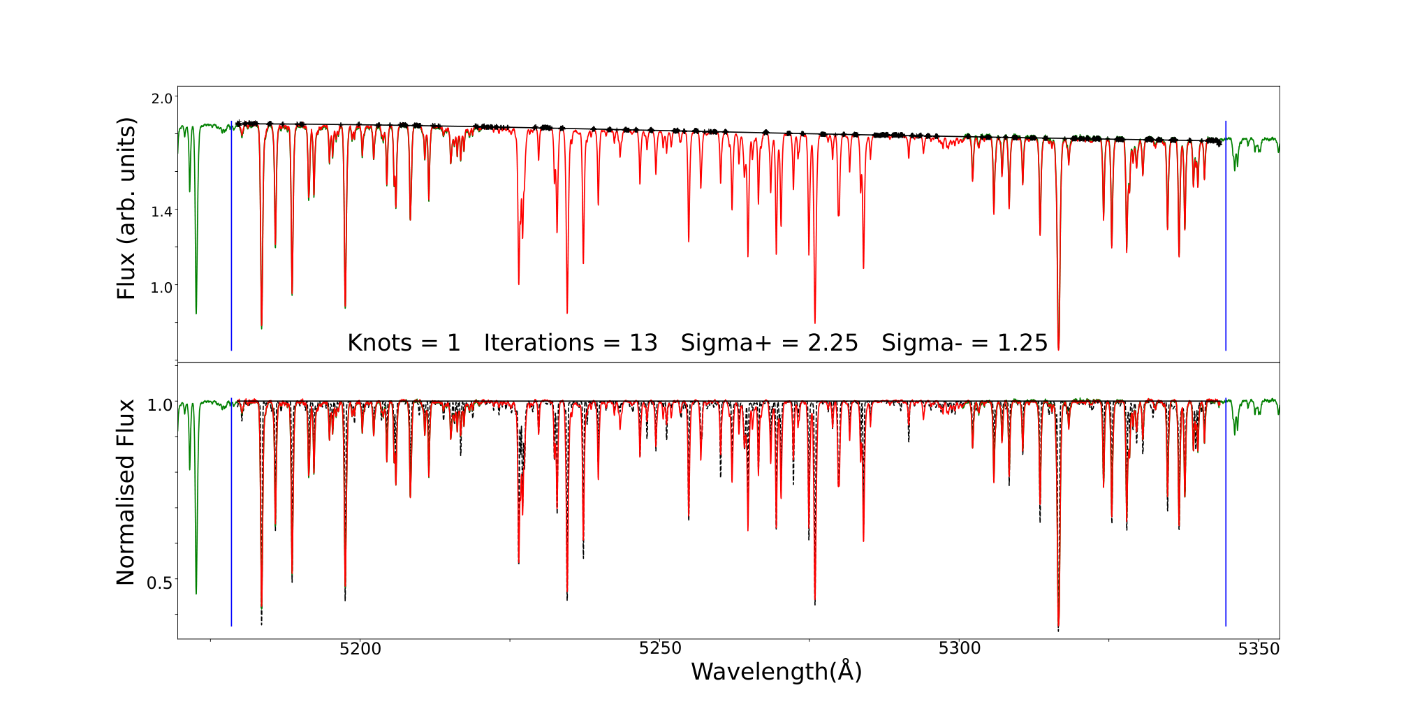
The LIFE project involves the analysis of a large number of spectra. Part of this analysis involves fitting the continuum of each spectral order for each observation to scale the stellar continuum to unity. Generally this is accomplished using IRAF, which is a very powerful tool. However, since we have such a large number of spectra our aim is to accomplish the normalisation in a semi-automatic way. As a result, we have developed a new code, spent (SPEctral Normalisation Tool), a python code which combines automatic sigma-clipping with adjustable edge regions in an interactive interface. An example of the graphical user interface of spent is shown in Fig. 9.
The code begins by fitting a third-order spline to one order of an unnormalised echelle spectrum. The points which make up the spectrum are then iteratively -clipped until the third order spline only passes through continuum points and so models the continuum. In this paper we only have absorption spectra, and so we must clip more points below the fit than above, to remove the absorption lines. However, the reverse is equally possible. The user is interactively able to define the number of interior knots used to calculate the spline fit, the number of iterations of the -clipping and the upper and lower threshold values. Each time a change is made to the parameters, the normalised spectrum is updated. For each star the normalisation parameters are saved in a log file, this means it is possible to fit future observations efficiently and consistently.
A key consideration when designing this code was that the edges of the orders of echelle spectrograph can occur in the middle of spectral lines. As a result it can be difficult to normalise these regions properly. To help overcome this issue, spent is built with two solutions. Firstly, the user is able to remove a number of points at either or both ends of the unnormalised spectral order. A cluster of points at the beginning and/or end of each order replaces these. This cluster can then be move up and down which artificially adjusts the end knots of the spline. The second solution is to show a portion of the spectral orders at each side of the currently active order. This makes it possible for the user to see the characteristics of the spectral line which has been split by the orders and compensate appropriately.