Efficient cubature rules

James R. Van Zandt Email: jrv@mitre.org Note: The MITRE Corporation, 202 Burlington Rd, Bedford, MA 01730. The author’s affiliation with The MITRE Corporation is provided for identification purposes only, and is not intended to convey or imply MITRE’s concurrence with, or support for, the positions, opinions or viewpoints expressed by the author.

Abstract

67 new cubature rules are found for three standard multidimensional integrals with spherically symmetric regions and weight functions, using direct search with a numerical zero-finder. 63 of the new rules have fewer integration points than known rules of the same degree, and 20 are within three points of Möller’s lower bound. Most have all positive coefficients and most have some symmetry, including some supported by one or two concentric spheres. They include degree 7 formulas for integration over the sphere and Gaussian-weighted integrals over all space, each in 6 and 7 dimensions, with 127 and 183 points, respectively.

1 Introduction

We are concerned with estimating multi-dimensional integrals of the form

\int_{\Omega}w({\bf x})f({\bf x})\;d{\bf x},

(1)

where ${\bf x}=[x_{1}\;x_{2}\cdots x_{n}]^{T}$ , for the integration regions $\Omega$ and weighting functions $w({\bf x})$ shown in Table 1. Applications of (1) include evaluation of quantum-mechanical matrix elements with Gaussian wave functions in atomic physics [1], nuclear physics [2], and particle physics [3]. For applications in statistics, particularly Bayesian inference, see [4]. For applications in target tracking, see [5, 6].

Table 1: Integrals Studied.

Name	Region $\Omega$	Weight Function $w({\bf x})$
$G_{n}$	entire space $\mathbb{R}^{n}$	(2 $\pi)^{-n/2}e^{-{\bf x}^{T}{\bf x}/2}$
$E_{n}^{r^{2}}$	entire space $\mathbb{R}^{n}$	$e^{-{\bf x}^{T}{\bf x}}$
$E_{n}^{r}$	entire space $\mathbb{R}^{n}$	$e^{-\sqrt{{\bf x}^{T}{\bf x}}}$
$S_{n}$	unit $n$ -sphere ${\bf x}^{T}{\bf x}\leq 1$	1

We approximate these integrals using cubature formulas or integration rules of the form

\sum_{i=1}^{N}W_{i}f({\bf x}_{i}),

(2)

where the weights $W_{i}$ and nodes or points ${\bf x}_{i}$ are independent of the function $f$ .

The first two integrals in the table are of course closely related. Given an approximation of $G_{n}$ of the form (2), we can construct an equivalent approximation $E_{n}^{r^{2}}\approx\sum_{i=1}^{N}B_{i}f({\bf b}_{i})$ where ${\bf b}_{i}={\bf x}_{i}/\sqrt{2}$ and $B_{i}=\pi^{n/2}W_{i}$ . In this paper we address $E_{n}^{r^{2}}$ , following the numerical analysis convention. However, in the supplemental material we quote the parameters for the corresponding $G_{n}$ formulas for the convenience of researchers using the other convention.

If an integration rule is exact for all polynomials up to and including degree $d$ , but not for some polynomial of degree $d+1$ , then we say the rule has algebraic degree of exactness (or simply degree) $d$ .

One can construct cubature formulas exact for a space of polynomials by solving the large system of polynomial equations associated with it. In describing this method, Cools stated that “it is essential to restrict the search to cubature formulas with a certain structure” [7]. For example, in [8, “CUT4” formulas], points were assumed to take the form

\begin{array}[]{rrrrr@{}lcc}(0,&0,&\cdots&0,&0&)&W_{0}&1\\ (\pm\eta,&0,&\cdots&0,&0&)_{S}&W_{1}&2n\\ (\pm\nu,&\pm\nu,&\cdots&\pm\nu,&\pm\nu&)&W_{2}&2^{n}\end{array}

(3)

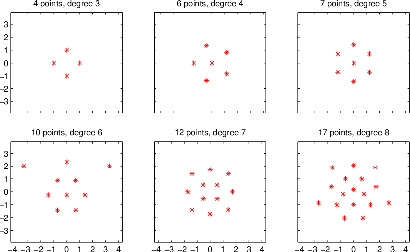
where the notation $(\cdots)_{S}$ indicates that all points obtained from these by permutation of coordinates are included, and are assigned the same weight. The last column gives the number of points. This point set is fully symmetric; i.e., closed under all coordinate permutations and sign changes. However, relaxing this symmetry requirement can allow us to find formulas with fewer points [9, 10]. For example (as shown in Figure 5), in two dimensions, there is a formula of degree five with points at the vertices of a regular hexagon [11, formula V], which is closed under sign permutations but not coordinate permutations. There is also a formula of degree 4 with points at the vertices of a regular pentagon, which is closed under sign changes in $x_{1}$ but not $x_{2}$ ; i.e., bilateral symmetry.

The objective of this work was to test whether the continuing improvements in computer processing have made the ‘‘brute force’’ approach---using a numerical zero-finder to solve the moment constraint equations directly, making few or no assumptions about the form of the points---feasible for interesting problems. We find that, for rules with up to approximately 3000 free parameters¹¹ 1 Each of the $N$ points has $n$ coordinates and a weight, so a rule has $(n+1)N$ free parameters., it is no longer necessary to assume at the outset that the points have a particular structure. Relieving those assumptions has made it possible to discover rules with fewer points than known rules of the same degree, including twenty rules that come within three points of the lower bound found by Möller [12, 13].

Section 2 describes our search method. Even a symmetric rule found by this method will have a random orientation, making it inconvenient to present and use. Section 3.1 describes how the description of a rule can be simplified by orienting it to take best advantage of any symmetries. Many of the rules found have little or no symmetry. Section 3.3 describes several procedures that can improve such a rule. Sections 4 through 10 present the new rules that have significant symmetry. Section 11 lists and discusses all the new rules. The supplemental material includes tables in double and quad precision of all the new rules, including those with little or no symmetry.

2 Searching

An approximation is exact for all polynomials with degree $\leq d$ if it is exact for all monomials

f({\bf x})=x_{1}^{\alpha_{1}}x_{2}^{\alpha_{2}}\cdots x_{n}^{\alpha_{n}},\quad 0\leq\alpha_{1}+\cdots+\alpha_{n}\leq d,

(4)

where the $\alpha_{i}$ are all nonnegative integers. If any of the $\alpha_{i}$ are odd, then the monomial integral is zero for any of our problems. Let $\bm{\alpha}=[\alpha_{1}\;\alpha_{2}\cdots\alpha_{n}]^{T}$ , where all $\alpha_{i}$ are even, and $\beta_{i}=(\alpha_{i}+1)/2$ . Then the monomial integral is [14, 11, 15]

\begin{array}[]{l@{\;}l}I(\bm{\alpha})&\equiv\int_{\Omega}w({\bf x})x_{1}^{\alpha_{1}}x_{2}^{\alpha_{2}}\cdots x_{n}^{\alpha_{n}}\;dx_{1}\;dx_{2}\;\cdots\;dx_{n}\\ \\ &=\left\{\begin{array}[]{rl}\Gamma(\beta_{1})\Gamma(\beta_{2})\cdots\Gamma(\beta_{n})&\hbox{for $E_{n}^{r^{2}}$}\\ {\displaystyle 2(\alpha_{1}+\cdots+\alpha_{n}+n-1)!\over\displaystyle\Gamma(\beta_{1}+\cdots+\beta_{n})}\Gamma(\beta_{1})\Gamma(\beta_{2})\cdots\Gamma(\beta_{n})&\hbox{for $E_{n}^{r}$}\\ {\displaystyle 1\over\displaystyle\Gamma(\beta_{1}+\cdots+\beta_{n}+1)}\Gamma(\beta_{1})\Gamma(\beta_{2})\cdots\Gamma(\beta_{n})&\hbox{for $S_{n}$}\quad.\\ \end{array}\right.\end{array}

(5)

For example, a rule of degree 4 for $E_{2}^{r^{2}}$ must satisfy these 15 constraints, where $x_{ij}$ is the $j$ th coordinate of the $i$ th point and each sum is over $i=1\ldots N$ :

\begin{array}[]{lllll}\sum W_{i}=\pi&\sum W_{i}x_{i1}=0&\sum W_{i}x_{i1}^{2}=\pi/2&\sum W_{i}x_{i1}^{3}=0&\sum W_{i}x_{i1}^{4}=3\pi/4\\[4.30554pt] \sum W_{i}x_{i2}=0&\sum W_{i}x_{i1}x_{i2}=0&\sum W_{i}x_{i1}^{2}x_{i2}=0&\sum W_{i}x_{i1}^{3}x_{i2}=0\\[4.30554pt] \sum W_{i}x_{i2}^{2}=\pi/2&\sum W_{i}x_{i1}x_{i2}^{2}=0&\sum W_{i}x_{i1}^{2}x_{i2}^{2}=\pi/4\\[4.30554pt] \sum W_{i}x_{i2}^{3}=0&\sum W_{i}x_{i1}x_{i2}^{3}=0\\[4.30554pt] \sum W_{i}x_{i2}^{4}=3\pi/4\end{array}

(6)

The number of constraints increases rapidly with $n$ and $d$ . The rules in Section 8.2 of dimension and degree 7 satisfy 3432 constraints.

Stroud [16] showed that if there is an $N$ point formula in $n$ dimensions of degree $d$ , then

N\geq{n+\lfloor d/2\rfloor\choose\lfloor d/2\rfloor},

(7)

Möller improved this bound for odd degrees [12, 13]. Let $d=2s-1$ , then

N\geq N_{MLB}\equiv\left\{\begin{array}[]{ll}{n+s-1\choose n}+\sum_{k=1}^{n-1}2^{k-n}{k+s-1\choose k}&s\hbox{ even}\\[4.30554pt] {n+s-1\choose n}+\sum_{k=1}^{n-1}(1-2^{k-n}){k+s-2\choose k}&s\hbox{ odd}\quad.\end{array}\right.

(8)

However, a formula satisfying the bound exactly may not exist. We searched for the rule of a given degree with the fewest points, using a binary search between Möller’s lower bound and the number of points in a known formula of the given degree or of the next higher degree.

We initialized each search with normally distributed points, assigning initial weights of

{\bf W}=e^{-\sqrt{{\bf x}^{T}{\bf x}}},

(9)

but then normalizing them so they sum to V:

V\equiv\int_{\Omega}w({\bf x})\;dx_{1}\;dx_{2}\;\cdots\;dx_{n}=\left\{\begin{array}[]{rl}\pi^{n/2}&\hbox{for $E_{n}^{r^{2}}$}\\ {\displaystyle 2(n-1)!\pi^{n/2}\over\displaystyle\Gamma(n/2)}&\hbox{for $E_{n}^{r}$}\\[6.45831pt] {\displaystyle 2\pi^{n/2}\over\displaystyle n\Gamma(n/2)}&\hbox{for $S_{n}$}\quad,\end{array}\right.

(10)

so the zeroth order constraint was satisfied exactly. The points were then linearly scaled so the second order constraints were also satisfied.

In most cases, the number of equations and unknowns were unequal (with almost all problems becoming over-determined before $N$ reached Möller’s lower bound), so many of the methods developed for solving nonlinear equations could not be applied. We used fsolve from the MATLAB Optimization Toolbox [17, 18, 19], or UDL²² 2 We revised UDL by adding a stopping criterion: If, after any seven consecutive steps, the norm of the residual has decreased by less than seven percent, then the search is deemed a failure. by Simonis [20]. After a failed search, we restarted with a new set of points. After a success, we tried dropping low-weight points, combining points with very near neighbors, and simply restarting with fewer points.

In a few cases, an elegant formula was found easily—with the weights on any extra points reduced to zero. However, ordinarily with extra points, and often even with no extra points, there are enough extra degrees of freedom that any symmetry is lost, and successive searches would find substantially different formulas. In those cases, additional constraints were added — moment constraints of the next higher degree, starting with

\sum_{i=1}^{N}W_{i}x_{ij}^{d+1}=I([d+1\;0\ldots 0]^{T}),

(11)

for $1\leq i\leq k\leq n$ .

Parameters of all searches were logged, along with the results of all successful searches; so the results of a lucky random starting point would not be lost. After finding a rule for one of the integrals, we also searched for similar rules for each of the other integrals, starting with the same point layout and relative weights, but normalizing the weights and scaling those points so its zeroth and second degree constraints were satisfied exactly.

3 Presentation

3.1 Rotations

One a rule is found, the first step is to sort the points by radius. If the rule is symmetric, as evidenced by several points at the same radius and with equal weights, it is desirable to determine its structure and if possible to express it in a simple form. Any orthogonal transformation of a set of points yields an equivalent set of points. Note that any orthogonal transformation can be expressed in terms of a skew-symmetric matrix via the Cayley transform [21]. Thus, in $n$ dimensions we have $n(n-1)/2$ free parameters we can use to orient a rule. Often we concentrate on the sphere supporting the fewest points, and we want to rotate to put one of those points on the first coordinate axis. Choosing points in that shell by increasing angular distance from that first point, we rotate to put a second point in the plane defined by the first two axes, a third point in the subspace defined by the first three axes, etc. We call this “aligning the axes” to the chosen points. Our process is as follows:

Assume we have chosen $n$ points. Reorder the rows of the point matrix so those rows appear in order at the top, forming a $n\times n$ submatrix we will call $A$ . The remainder of the rows form a submatrix we will call $B$ . Use the QR decomposition to factor the transpose of $A$ , so that

A^{T}=RU,

(12)

where $R$ is orthogonal and $U$ is upper triangular. Taking the transpose of both sides, we have

A=(RU)^{T}=U^{T}R^{T},

(13)

and right multiplying by $R$ we have

AR=U^{T}R^{T}R=U^{T}.

(14)

Thus, right multiplying our original point matrix by $R$ gives us

\left[\begin{array}[]{c}A\\ B\end{array}\right]R=\left[\begin{array}[]{c}U^{T}\\ C\end{array}\right].

(15)

$U^{T}$ is lower triangular. In its first row, only the first element is nonzero, so it represents a point along the first coordinate. In the second row, only the first two elements are nonzero, etc. This satisfies the requirements set out above.

If a rule in $n$ dimensions has $n+1$ points at the same radius (such as the 6 inner points in the 5 dimensional rules of Section 5.4), they typically appear at the vertices of a regular $n$ simplex. In that case, a simple description can be found by rotating one point to be equidistant from all coordinate axes, with each of the other $n$ points in the plane defined by that first point and one of the coordinate axes.

3.2 Closed form expressions

If a rule has enough symmetry, we attempt to express its points and weights in closed form. In some cases they are integers, simple fractions, or square roots of simple fractions, which can be identified by converting them to a simple continued fraction and looking for a repeating pattern [22]. To guard against mathematical coincidences, our next step is to use Maxima [23, 24] to confirm that the resulting rule satisfies the moment constraint equations exactly, or (if Maxima could not simplify some expressions) with absolute error less than $10^{-55}$ .

We also attempted to identify the points as vertices of some known polytope. This allows the points to be described economically and calculated directly.

3.3 Economizing

A rule lacking any symmetry was assumed to have extra degrees of freedom, even if it had the minumum number of points. We tried improving its symmetry by projecting the innermost or outermost few points to (or toward) the same radius, giving them all the same weight, and using that revised configuration to start a new search. In a few cases, this enabled us to eliminate negative weights or drop some points.

We similarly tried to impose bilateral symmetry. We reoriented the rule so eigenvectors of the covariance of the unweighted points were aligned with the coordinate axes. We then tested whether the rule was close to bilaterally symmetric with respect to any of the axes. If so, we searched for a similar symmetric rule.

Initially, we simply sorted the points along that coordinate value, pairing the first with the last, the second with the next to last, etc. For each pair, we moved the points to be exactly symmetric (i.e., moving each to the mean of its own position and that of the reflection of the associated point) and gave each the mean of the two original weights. Points near the symmetry plane were moved to that plane. This simple method failed when the initial positions were far enough away from symmetry (e.g., if the eigenvectors did not match the symmetry plane well enough) to change the ordering of the points along the chosen axis.

Eventually we switched to treating the association of the original and reflected points as a linear assignment problem, solving it with the Jonker-Volgenant-Castanon (JVC) assignment algorithm [25, 26], This had the additional benefit of eliminating the need for a threshold for being “near” the symmetry plane. If a point were assigned to its own reflection, then its adjusted position would automatically be on the symmetry plane.

4 Degree 2 rules

The classical second degree rules have $n+1$ points at the vertices of an $n$ simplex. They are usually presented in the form [15, 27, 28]

\chi=\sqrt{n+1}\left[\begin{array}[]{ccccc}\sqrt{1\over 1\cdot 2}&\sqrt{1\over 2\cdot 3}&\sqrt{1\over 3\cdot 4}&\cdots&\sqrt{1\over n(n+1)}\\ -\sqrt{1\over 1\cdot 2}&\sqrt{1\over 2\cdot 3}&\sqrt{1\over 3\cdot 4}&\cdots&\sqrt{1\over n(n+1)}\\ 0&-\sqrt{2\over 3}&\sqrt{1\over 3\cdot 4}&\cdots&\sqrt{1\over n(n+1)}\\ 0&0&-\sqrt{3\over 4}&\cdots&\sqrt{1\over n(n+1)}\\ \vdots&\vdots&\vdots&\ddots&\sqrt{1\over n(n+1)}\\ 0&0&0&\cdots&-\sqrt{n\over n+1}\end{array}\right],

(16)

where each row represents a point, and the weight on each point is $1/(n+1)$ . Fan and You noticed that in three dimensions the points can be expressed in the much simpler form [29]

\chi=\left[\begin{array}[]{rrrr}1&1&1\\ 1&-1&-1\\ -1&1&-1\\ -1&-1&1\end{array}\right].

(17)

This can be generalized to other dimensions, yielding the set of points

\chi=\left[\begin{array}[]{cccccc}1&1&1&\cdots&1\\ a&b&b&\cdots&b\\ b&a&b&\cdots&b\\ b&b&a&\cdots&b\\ \vdots&\vdots&\vdots&\ddots&\vdots\\ b&b&b&\cdots&a\end{array}\right],

(18)

with the two solutions

a={-1+{\left(n-1\right)\,\sqrt{n+1}}\over{n}},\qquad b={-1-{\sqrt{n+1}}\over{n}},

(19)

a={-1-{\left(n-1\right)\,\sqrt{n+1}}\over{n}},\qquad b={-1+{\sqrt{n+1}}\over{n}}.

(20)

When a rule has $n+1$ points at the vertices of a regular simplex, it can be rotated into one of these orientations.

5 Degree 4 rules

5.1 Degree 4, dimension 3, 10 point rules

The points in these new formulas for $E_{3}^{r^{2}}$ and $S_{3}$ are closed with respect to sign changes along two of the three coordinates. The points form two pyramids, with one offset and rotated from the other, as shown in Figure 1. The configuration is shown in Table 2. The Maxima program verifying the correctness of these rules is shown in Figure 2. The supplemental material includes similar programs for the other new rules.

Becker found an 11 point cubature formula of degree 4 for $S_{3}$ [30], but we are not aware of any previous formulas of degree 4 for $E_{3}^{r^{2}}$ .

Refer to caption — Figure 1: Configuration of the 10 points for the rule of degree 4 for $E_{3}^{r^{2}}$ .

Table 2: 10 Point Rules of Degree 4 for

E_{3}^{r^{2}}

and

S_{3}

$x_{1}$	$x_{2}$	$x_{3}$		Weight	# Points
$g$	0	0		$W_{3}$	1
$a$	$(\pm c$	0	$)_{S}$	$W_{2}$	4
$-b$	0	0		$W_{1}$	1
$-e$	$\pm f$	$\pm f$		$W_{4}$	4

	$E_{3}^{r^{2}}\rule{0.0pt}{11.19443pt}$	$S_{3}$
$a$	$(\sqrt{3}-1)/2\rule{0.0pt}{11.19443pt}$	$(2\sqrt{3}-1)/\sqrt{77}$
$b$	$(\sqrt{7}-1)/2$	$(2\sqrt{203}-\sqrt{77})/35$
$c$	$\sqrt{3-\sqrt{3}}$	$\sqrt{(48-8\sqrt{3})/77}$
$e$	$(\sqrt{3}+1)/2$	$(2\sqrt{3}+1)/\sqrt{77}$
$f$	$\sqrt{(\sqrt{3}+3)/2}$	$\sqrt{(24+4\sqrt{3})/77}$
$g$	$(\sqrt{7}+1)/2$	$(2\sqrt{203}+\sqrt{77})/35$
$W_{1}$	$\pi^{3/2}\,(2\,\sqrt{7}+7)/42$	$\pi(841+32\sqrt{11}\sqrt{29})/5220$
$W_{2}$	$\pi^{3/2}\,(\sqrt{3}+2)/24$	$7\pi(13+4\sqrt{3})/720$
$W_{3}$	$\pi^{3/2}\,(7-2\,\sqrt{7})/42$	$\pi(841-32\sqrt{11}\sqrt{29})/5220$
$W_{4}$	$\pi^{3/2}\,(2-\sqrt{3})/24$	$7\pi(13-4\sqrt{3})/720$

rule:"3_10_4"; n:3; N:10; deg:4; /* 3 dimensions, 10 points, degree 4 */
/*            G_n                        E_nˆ{rˆ2}                S_n */
a_vals:[(sqrt(6)-sqrt(2))/2 ,(sqrt(6)-sqrt(2))/sqrt(8) ,0,(2*sqrt(3)-1)/sqrt(77)         ];
b_vals:[(sqrt(14)-sqrt(2))/2,(sqrt(14)-sqrt(2))/sqrt(8),0,(2*sqrt(203)-sqrt(77))/35      ];
c_vals:[sqrt(6 - 2*sqrt(3)) ,sqrt((6 - 2*sqrt(3))/2)   ,0,sqrt((48-8*sqrt(3))/77)        ];
e_vals:[(sqrt(6)+sqrt(2))/2 ,(1+sqrt(3))/2             ,0,(2*sqrt(3)+1)/sqrt(77)         ];
f_vals:[sqrt(sqrt(3)+3)     ,sqrt((sqrt(3)+3)/2)       ,0,sqrt((24+4*sqrt(3))/77)        ];
g_vals:[(1+sqrt(7))/sqrt(2) ,(1+sqrt(7))/2             ,0,(2*sqrt(203)+sqrt(77))/35      ];
w1vals:[(7+2*sqrt(7))/42,%piˆ(3/2)*(2*sqrt(7)+7)/42,0,%pi*(841+32*sqrt(11)*sqrt(29))/5220];
w2vals:[(sqrt(3)+2)/24  ,%piˆ(3/2)*(sqrt(3)+2)/24  ,0,%pi*(13+4*sqrt(3))*7/720           ];
w3vals:[(7-2*sqrt(7))/42,%piˆ(3/2)*(7-2*sqrt(7))/42,0,%pi*(841-32*sqrt(11)*sqrt(29))/5220];
w4vals:[(2-sqrt(3))/24  ,%piˆ(3/2)*(2-sqrt(3))/24  ,0,%pi*(13-4*sqrt(3))*7/720           ];
plabel:["       Gn","E_nˆ{rˆ2}","      E_n","       Sn"];
for problem in [1,2,4] do block(
a: a_vals[problem],
b: b_vals[problem],
c: c_vals[problem],
e: e_vals[problem],
f: f_vals[problem],
g: g_vals[problem],
w1:w1vals[problem],
w2:w2vals[problem],
w3:w3vals[problem],
w4:w4vals[problem],
x:matrix([ g, 0, 0, w3],
         [ a, c, 0, w2],
         [ a,-c, 0, w2],
         [ a, 0, c, w2],
         [ a, 0,-c, w2],
         [-b, 0, 0, w1],
         [-e, f, f, w4],
         [-e, f,-f, w4],
         [-e,-f, f, w4],
         [-e,-f,-f, w4]),
ex(a,p) := if p=0 then 1 else aˆp,
alpha : makelist(0,i,n),
pass : true,
for i1 : 0 thru deg do
  (alpha[1] : i1,
  for i2 : 0 thru deg-i1 do
    (alpha[2] : i2,
    for i3 : 0 thru deg-i1-i2 do
      (alpha[3] : i3,
        if sum(alpha[i],i,1,n)<=deg then
        (beta : (alpha+makelist(1,i,n))/2,
          odd : false, for i : 1 thru n do odd : odd or oddp(alpha[i]),
  m :  if odd then 0 else
       if problem=1 then 2ˆsum(beta[ii],ii,1,n)*product(gamma(beta[ii]),ii,1,n)
         /(2*%pi)ˆ(n/2) else
       if problem=2 then product(gamma(beta[ii]),ii,1,n) else
       if problem=3 then 2*gamma(sum(alpha[ii],ii,1,n)+n)
         *product(gamma(beta[ii]),ii,1,n)/gamma(sum(beta[ii],ii,1,n)) else
       if problem=4 then product(gamma(beta[ii]),ii,1,n)/sum(beta[ii],ii,1,n)
         /gamma(sum(beta[ii],ii,1, else
       if problem=5 then 2*product(gamma(beta[ii]),ii,1,n)
          /gamma(sum(beta[ii],ii,1,n)),
          value : radcan(sum(product(ex(x[i,j],alpha[j]),j,1,n)*x[i,n+1],i,1,N)),
          subtest : value=m, /* test one constraint */
          pass : pass and subtest)))),
print(plabel[problem],":",rule,"...", if pass then "pass" else "FAIL" ))$

Figure 2: The Maxima program (m3_10_4.mac) verifying the correctness of the rules of degree 4 in 3 dimensions.

5.2 Degree 4, dimension 3, 11 point rule

We were unable to find a 10 point rule for $E_{3}^{r}$ , but we did find the 11 point rule shown in Table 3. This rule has at least one remaining degree of freedom, as the $x_{3}$ coordinate in the fourth line of the table need not be zero. An example with a nonzero value appears in the supplemental material.

Table 3: 11 Point Rule of Degree 4 for

E_{3}^{r}

$x_{1}$	$x_{2}$	$x_{3}$	Weight
$\pm$ 5.123512671436	4.925613098468	0.000000000000	0.379658096396
$\pm$ 4.102816292737	-1.218122471265	1.544992698170	1.815112382679
$\pm$ 3.636092685910	-1.218122471265	-4.843920857272	0.737101279022
0.000000000000	-1.836923221948	0.000000000000	8.813498359176
0.000000000000	-12.639707409137	-3.423767380484	0.036648025338
0.000000000000	1.948389609086	-1.422580596634	7.054048788228
0.000000000000	1.703608086180	3.398957047139	3.331366718822
0.000000000000	-8.635010968135	11.051160549267	0.033435820963

5.3 Degree 4, dimension 4, 16 point rules

We found two sets of 16 point rules. Those in the first set have a central point, one shell of 10 points, and another shell of 5 points, as shown in Table 4. The formula for $S_{4}$ has five points outside the region, and one with a negative weight.

Table 4: 16 Point Rules of Degree 4 in 4 Dimensions (Group 1).

$x_{1}$	$x_{2}$	$x_{3}$	$x_{4}$		Weight	Radius	# Points
0	0	0	0		$W_{0}$	0	1
$(c$	$c$	$-b$	$-b$	$)_{S}$	$W_{1}$	$r_{1}$	6
$(-e$	$-a$	$-a$	$-a$	$)_{S}$	$W_{1}$	$r_{1}$	4
$f$	$f$	$f$	$f$		$W_{2}$	$r_{2}$	1
$(g$	$-e$	$-e$	$-e$	$)_{S}$	$W_{2}$	$r_{2}$	4

	$E_{4}^{r^{2}}\rule{0.0pt}{11.19443pt}$	$E_{4}^{r}$	$S_{4}$
$a$	$(3\sqrt{3}-\sqrt{15})/12\rule{0.0pt}{11.19443pt}$	$(3\sqrt{42}-\sqrt{210})/12$	$(3\sqrt{3}-\sqrt{15})/24$
$b$	$(\sqrt{15}-\sqrt{3})/6$	$(\sqrt{210}-\sqrt{42})/6$	$(\sqrt{15}-\sqrt{3})/12$
$c$	$(\sqrt{15}+\sqrt{3})/6$	$(\sqrt{210}+\sqrt{42})/6$	$(\sqrt{15}+\sqrt{3})/12$
$e$	$(\sqrt{15}+\sqrt{3})/4$	$(\sqrt{210}+\sqrt{42})/4$	$(\sqrt{15}+\sqrt{3})/8$
$f$	$\sqrt{3}$	$\sqrt{42}$	$\sqrt{3}/2$
$g$	$(3\sqrt{15}-\sqrt{3})/4$	$(3\sqrt{210}-\sqrt{42})/4$	$(3\sqrt{15}-\sqrt{3})/8$
$W_{0}$	$\pi^{2}/12$	$29\pi^{2}/7$	$-\pi^{2}/9$
$W_{1}$	$9\pi^{2}/100$	$27\pi^{2}/35$	$3\pi^{2}/50$
$W_{2}$	$\pi^{2}/300$	$\pi^{2}/35$	$\pi^{2}/450$
$r_{1}$	$\sqrt{2}$	$\sqrt{28}$	$\sqrt{1/2}$
$r_{2}$	$\sqrt{12}$	$\sqrt{168}$	$\sqrt{3}$

Each rule in the second set has a central point, a shell of 6 points, and another shell of 9 points, as shown in Table 5. The second formula for $S_{4}$ has zero weight on the central point, making it a 15 point formula, with all positive weights and nine points on the boundary.

Both of these formulas for $S_{4}$ are distinct from the 16 point formula found by Mysovskih [31, 32] which has positive weights and seven points on the boundary. We are not aware of previous degree 4 formulas for the other integrals.

Table 5: 16 or 15 Point Rules of Degree 4 in 4 Dimensions (Group 2).

$x_{1}$	$x_{2}$	$x_{3}$	$x_{4}$	Weight	Radius	# Points
0	0	0	0	$W_{0}$	0	1
0	0	0	$-c$	$W_{1}$	$r_{1}$	1
0	0	$c$	0	$W_{1}$	$r_{1}$	1
$\pm b$	0	$-a$	0	$W_{1}$	$r_{1}$	2
0	$\pm b$	0	$a$	$W_{1}$	$r_{1}$	2
$\pm b$	$\pm b$	$a$	$-a$	$W_{2}$	$r_{2}$	4
0	$\pm b$	$-c$	$-a$	$W_{2}$	$r_{2}$	2
$\pm b$	0	$a$	$c$	$W_{2}$	$r_{2}$	2
0	0	$-c$	$c$	$W_{2}$	$r_{2}$	1

	$E_{4}^{r^{2}}$	$E_{4}^{r}$	$S_{4}$
$a$	$\sqrt{1/2}$	$\sqrt{7}$	$\sqrt{1/8}$
$b$	$\sqrt{3/2}$	$\sqrt{21}$	$\sqrt{3/8}$
$c$	$\sqrt{2}$	$\sqrt{28}$	$\sqrt{1/2}$
$W_{0}$	$\pi^{2}/4$	$39\pi^{2}/7$	0
$W_{1}$	$\pi^{2}/12$	$5\pi^{2}/7$	$\pi^{2}/18$
$W_{2}$	$\pi^{2}/36$	$5\pi^{2}/21$	$\pi^{2}/54$
$c=r_{1}$	$\sqrt{2}$	$\sqrt{28}$	$\sqrt{1/2}$
$r_{2}$	2	$\sqrt{56}$	1

5.4 Degree 4, dimension 5, 22 point rules

Each of these new formulas has a central point and two shells. We can describe the points using five generators, as shown in Table 6. The six points with weight $W_{0}$ are at the vertices of a regular 5-simplex. The 15 points with weight $W_{1}$ are the vertices of a rectified 5-simplex; i.e., each vertex being at the center of an edge of a regular 5-simplex. A MATLAB program to generate these rules (c5_22_4.m) is included in the supplemental materials.

Table 6: 22 Point Rules of Degree 4 in 5 Dimensions.

$x_{1}$	$x_{2}$	$x_{3}$	$x_{4}$	$x_{5}$		Weight	# Points
0	0	0	0	0		$W_{0}$	1
$c$	$c$	$c$	$c$	$c$		$W_{1}$	1
$(-h$	$a$	$a$	$a$	$a$	$)_{S}$	$W_{1}$	5
$(-b$	$-b$	$-b$	$g$	$g$	$)_{S}$	$W_{2}$	10
$(e$	$-f$	$-f$	$-f$	$-f$	$)_{S}$	$W_{2}$	5

	$E_{5}^{r^{2}}\rule{0.0pt}{11.19443pt}$	$E_{5}^{r}$	$S_{5}$
$a\rule{0.0pt}{11.19443pt}$	$(2\sqrt{3}-\phantom{2}\sqrt{2})/10$	$(\phantom{1}4\sqrt{3}-2\sqrt{2})/5$	$(\phantom{2}\sqrt{6}-1)/15$
$b$	$(2\sqrt{3}-\phantom{2}\sqrt{2})/5$	$(\phantom{1}8\sqrt{3}-4\sqrt{2})/5$	$(2\sqrt{6}-2)/15$
$c$	$\sqrt{1/2}$	$\sqrt{8}$	$1/3$
$e$	$(4\sqrt{3}-2\sqrt{2})/5$	$(16\sqrt{3}-8\sqrt{2})/5$	$(4\sqrt{6}-4)/15$
$f$	$(\phantom{2}\sqrt{3}+2\sqrt{2})/5$	$(\phantom{1}4\sqrt{3}+8\sqrt{2})/5$	$(\phantom{2}\sqrt{6}+4)/15$
$g$	$(3\sqrt{3}+\phantom{2}\sqrt{2})/5$	$(12\sqrt{3}+4\sqrt{2})/5$	$(3\sqrt{6}+2)/15$
$h$	$(8\sqrt{3}+\phantom{2}\sqrt{2})/10$	$(16\sqrt{3}+2\sqrt{2})/5$	$(4\sqrt{6}+1)/15$
$W_{0}$	$\pi^{5/2}/4$	$28\pi^{2}$	$2\pi^{2}/105$
$W_{1}$	$\pi^{5/2}/18$	$8\pi^{2}/3$	$4\pi^{2}/105$
$W_{2}$	$\pi^{5/2}/36$	$4\pi^{2}/3$	$2\pi^{2}/105$
$r_{1}$	$\sqrt{5/2}$	$\sqrt{40}$	$\sqrt{5}/3$
$r_{2}$	$2$	$8$	$\sqrt{8}/3$

5.5 Degree 4, dimension 6, 28 point rules

Each of these new formulas has a central point and 27 points all at the same radius. The rule is shown in Table 7. Each point on the shell has 16 near neighbors ( 76 degrees away) and 10 more distant neighbors (120 degrees). This configuration is suggested in Figure 3, which shows the points in terms of their angular distance from a chosen point, though of course their distances from each other cannot be shown realistically.

Table 7: 28 Point Rules of Degree 4 in 6 Dimensions.

$x_{1}$	$x_{2}$	$x_{3}$	$x_{4}$	$x_{5}$	$x_{6}$		Weight	Radius	# Points
0	0	0	0	0	0		$W_{0}$	0	1
$-c$	$\pm e$	0	0	0	0		$W_{1}$	$r$	2
$-c$	0	$\pm(b$	$b$	$b$	$-b$	$)_{S}$	$W_{1}$	$r$	8
$a$	$-b$	$\pm(b$	$b$	$b$	$b$	)	$W_{1}$	$r$	2
$a$	$-b$	$(b$	$b$	$-b$	$-b$	$)_{S}$	$W_{1}$	$r$	6
$f$	0	0	0	0	0		$W_{1}$	$r$	1
$a$	$b$	$\pm(e$	0	0	0	$)_{S}$	$W_{1}$	$r$	8

	$E_{6}^{r^{2}}\rule{0.0pt}{11.19443pt}$	$E_{6}^{r}$	$S_{6}$
$a$	$1/2$	$\sqrt{9/2}$	$\sqrt{1/20}$
$b$	$\sqrt{3/4}$	$\sqrt{27/2}$	$\sqrt{3/20}$
$c$	$1$	$\sqrt{18}$	$\sqrt{1/5}$
$e$	$\sqrt{3}$	$\sqrt{54}$	$\sqrt{3/5}$
$f=r$	$2$	$\sqrt{72}$	$\sqrt{4/5}$
$W_{0}$	$\pi^{3}/4$	$50\pi^{3}$	$\pi^{3}/96$
$W_{1}$	$\pi^{3}/36$	$70\pi^{3}/27$	$5\pi^{3}/864$

5.6 Degree 4, dimension 7, 38 point rules

We found 38 point rules for $E_{7}^{r^{2}}$ and $S_{7}$ , each with two negative weights. A standard measure of the stability of an integration rule is the sum of the absolute value of the weights, divided by the sum of the weights, which is a worst-case round-off error magnification factor [33]. These rules have stability factors of 7.18 for $E_{7}^{r^{2}}$ and 8.55 for $S_{7}$ . They have some symmetry, with the center point, a centered shell of 21 points, and two offset irregular 7-simplices. The configuration of the points with respect to one of the negative weight points is suggested in Figure 4. The rules are shown in Table 8.

Table 8: 38 Point Rules of Degree 4 in 7 Dimensions.

$x_{1}$	$x_{2}$	$x_{3}$	$x_{4}$	$x_{5}$	$x_{6}$	$x_{7}$		Weight	# Points
0	0	0	0	0	0	0		$\phantom{-}W_{0}$	1
$c$	$c$	$c$	$c$	$c$	$c$	$c$		$-W_{2}$	1
$-b$	$-b$	$-b$	$-b$	$-b$	$-b$	$-b$		$-W_{1}$	1
$(\hskip 4.30554ptf$	$-e$	$-e$	$-e$	$-e$	$-e$	$-e$	$)_{S}$	$\phantom{-}W_{3}$	7
$(\hskip 4.30554pth$	$a$	$a$	$a$	$a$	$a$	$a$	$)_{S}$	$\phantom{-}W_{4}$	7
$(-i$	$-i$	$g$	$g$	$g$	$g$	$g$	$)_{S}$	$\phantom{-}W_{5}$	21

	$E_{7}^{r^{2}}\rule{0.0pt}{11.19443pt}\hskip 25.00003pt$	$S_{7}$
$a$	0.2286166663871	0.0974824740891
$b$	0.2590817563916	0.1104728321147
$c$	0.3117777721419	0.1329424887288
$e$	0.4422503418055	0.1885761793629
$f$	0.4505846393780	0.1921299357884
$g$	0.7531484451994	0.3211435760773
$h$	1.0981884332902	0.4682691213418
$i$	1.8927504201541	0.8070714909185
$W_{0}$	59.8014451908073	5.2337832579847
$W_{1}$	89.9014937680773	9.4465413692728
$W_{2}$	79.9432767398149	8.4001659957515
$W_{3}$	11.6616239025637	1.2253635397056
$W_{4}$	11.0688850060780	1.1630805645052
$W_{5}$	0.2803313076587	0.0294562546617

6 Degree 5 rules

6.1 Degree 5, dimension 4, 23 point rules

This new family of degree 5 rules is shown in Table 9. Other than the central point, all points are at the same radius. However, two of those points have lower weight than the others. The rule for $E_{5}^{r}$ has fewer points than for the known rules. A 22 point rule of degree 5 was known for $S_{n}$ [15, $S_{n}$ :5-1].

Table 9: 23 Point Rules of Degree 5 in 4 Dimensions.

$x_{1}$	$x_{2}$	$x_{3}$		$x_{4}$	Weight	Radius	# Points
0	0	0		0	$W_{0}$	0	1
$\pm h$	0	0		0	$W_{2}$	$r$	2
0	$\pm h$	0		0	$W_{1}$	$r$	2
$\pm c$	$\pm(b$	$-a$	)	$\pm c$	$W_{1}$	$r$	8
$\pm c$	$\pm(b$	$e$	)	0	$W_{1}$	$r$	4
0	$\pm(a$	$-g$	)	0	$W_{1}$	$r$	2
0	$\pm(a$	$b$	)	$\pm f$	$W_{1}$	$r$	4

	$E_{4}^{r^{2}}\rule{0.0pt}{11.19443pt}$	$E_{4}^{r}$	$S_{4}$
$a$	$\sqrt{1/3}\rule{0.0pt}{11.19443pt}$	$\sqrt{14/3}$	$\sqrt{1/12}$
$b$	$\sqrt{2/3}$	$\sqrt{28/3}$	$\sqrt{1/6}$
$c$	$1$	$\sqrt{14}$	$\sqrt{1/4}$
$e$	$\sqrt{4/3}$	$\sqrt{56/3}$	$\sqrt{1/3}$
$f$	$\sqrt{2}$	$\sqrt{28}$	$\sqrt{1/2}$
$g$	$\sqrt{8/3}$	$\sqrt{112/3}$	$\sqrt{2/3}$
$h=r$	$\sqrt{3}$	$\sqrt{42}$	$\sqrt{3/4}$
$W_{0}$	$\pi^{2}/3$	$44\pi^{2}/7$	$\pi^{2}/18$
$W_{1}$	$\pi^{2}/32$	$15\pi^{2}/56$	$\pi^{2}/48$
$W_{2}$	$\pi^{2}/48$	$5\pi^{2}/28$	$\pi^{2}/72$

6.2 Degree 5, dimension 6, 44 point rule

This new rule has points supported by two spheres, as shown in Table 10.

Table 10: 44 Point Rule of Degree 5 for

E_{6}^{r}

$x_{1}$	$x_{2}$	$x_{3}$	$x_{4}$	$x_{5}$	$x_{6}$		Weight	Radius	# Points
(0	0	0	0	0	$\pm b$	$)_{S}$	$\phantom{-}W_{1}$	$r_{1}$	12
$(a$	$a$	$a$	$a$	$a$	$-a$	$)_{S}$	$\phantom{-}W_{2}$	$r_{2}$	6
$(a$	$a$	$a$	$-a$	$-a$	$-a$	$)_{S}$	$\phantom{-}W_{2}$	$r_{2}$	20
$(a$	$-a$	$-a$	$-a$	$-a$	$-a$	$)_{S}$	$\phantom{-}W_{2}$	$r_{2}$	6

	$E_{6}^{r}$
$a$	4.84099298434420
$b=r_{1}$	5.40578920173885
$W_{1}$	274.495347525855
$W_{2}$	13.3377822289287
$r_{2}$	11.8579626600364

7 Degree 6 rules

7.1 Degree 6, dimension 2, 10 point rule

A rule was found for $E_{2}^{r^{2}}$ with 10 points, achieving Stroud’s lower bound (7). This rule was known, but unpublished[34, 35]. The points and weights are shown in Table 11. The point layout is similar to that in the 10 point rule for $S_{2}$ by Wissmann and Becker [10, $S_{2}$ :6-1]. The points are shown in Figure 5, along with those for known formulas of degree 3, 4, 5, and 7, and the new formula of degree 8 discussed below. Note in the figure that the rules of odd degree have central symmetry (for every point $x$ , there is also a point $-x$ with the same weight), while those of even degree are only bilaterally symmetric.

Table 11: 10 Point Rule of Degree 6 for

E_{2}^{r^{2}}

$x_{1}$	$x_{2}$	Weight	Radius
$\pm$ 3.314013565941806	2.014171295633760	0.000757833922865	3.87809
$\pm$ 1.411670545911536	-0.242569904073576	0.236161927729435	1.43236
$\pm$ 0.713033732783175	-1.432390280414699	0.146082553662775	1.60005
$\pm$ 0.691608815107559	0.877693534044218	0.485399260031153	1.11744
0.000000000000000	-0.261367769356158	1.387418367858287	0.26137
0.000000000000000	2.335832264987514	0.017371135039050	2.33583

7.2 Degree 6, dimension 2, 11 point rule

This new rule for $E_{2}^{r}$ has 11 points, with bilateral symmetry. The points and weights are shown in Table 12. This rule come close to pentagonal symmetry, but we were unable to adjust it for pentagonal symmetry.

Table 12: 11 Point Rule of Degree 6 for

E_{2}^{r}

$x_{1}$	$x_{2}$	Weight	Radius
0.000000000000000	0.000000000000000	3.927702275194840	0.00000
0.000000000000000	10.299713185154499	0.003846684331349	10.29971
0.000000000000000	-3.895765525253948	0.474246212300936	3.89577
$\pm$ 10.311630315898372	3.397224688449697	0.002841012046587	10.85683
$\pm$ 6.251012172182811	-8.794364006109971	0.002944454683352	10.78962
$\pm$ 3.752487980256190	-1.228482827331175	0.460111970539923	3.94846
$\pm$ 2.312667676618243	3.141828043257887	0.472797630406369	3.90122

8 Degree 7 rules

We found four rules of degree 7 with fewer points than previously reported.

8.1 Degree 7, dimension 6, 127 point rules

Each of these new rules has a central point and two shells. The inner shell has 54 points. Each of those has 10 nearest neighbors in that shell (60 degrees away), and 16, 16, 10, and 1, successively further away. The outer shell has 72 points. Each of those has 20 nearest neighbors, and 30, 20, and 1, successively further away. The configuration of points is shown in Table 13.

Table 13: 127 Point Rules of Degree 7 in 6 Dimensions.

$x_{1}$	$x_{2}$	$x_{3}$	$x_{4}$	$x_{5}$	$x_{6}$		Weight	Radius	# Points
0	0	0	0	0	0		$W_{0}$	0	1
$\pm g$	0	0	0	0	0		$W_{1}$	$r_{1}$	2
$\pm c$	( $\pm f$	0	0	0	0	$)_{S}$	$W_{1}$	$r_{1}$	20
$\pm(a$	$b$	$b$	$b$	$b$	$b$	)	$W_{1}$	$r_{1}$	2
$\pm(a$	$(b$	$b$	$b$	$-b$	$-b$	$)_{S})$	$W_{1}$	$r_{1}$	20
$\pm(a$	$(b$	$-b$	$-b$	$-b$	$-b$	$)_{S})$	$W_{1}$	$r_{1}$	10
$\pm(h$	$(e$	$e$	$e$	$e$	$-e$	$)_{S})$	$W_{2}$	$r_{2}$	10
$\pm(h$	$(e$	$e$	$-e$	$-e$	$-e$	$)_{S})$	$W_{2}$	$r_{2}$	20
$\pm(h$	$-e$	$-e$	$-e$	$-e$	$-e$	)	$W_{2}$	$r_{2}$	2
0	$(\pm i$	$\pm i$	0	0	0	$)_{S}$	$W_{2}$	$r_{2}$	40

	$E_{6}^{r^{2}}\rule{0.0pt}{11.19443pt}$	$S_{6}$
$g=r_{1}$	$\sqrt{(4-\sqrt{6})\times 2}\rule{0.0pt}{13.77771pt}$	$\sqrt{2/3}$
$c$	$\sqrt{(4-\sqrt{6})/2}$	$\sqrt{1/6}$
$f$	$\sqrt{(4-\sqrt{6})\times 3/2}$	$\sqrt{1/2}$
$a$	$\sqrt{(4-\sqrt{6})/8}$	$\sqrt{1/24}$
$b$	$\sqrt{(4-\sqrt{6})\times 3/8}$	$\sqrt{1/8}$
$e$	$\sqrt{(6+\sqrt{6})/8}$	$\sqrt{1/8}$
$h$	$\sqrt{(6+\sqrt{6})\times 3/8}$	$\sqrt{3/8}$
$i$	$\sqrt{(6+\sqrt{6})/2}$	$\sqrt{1/2}$
$r_{2}$	$\sqrt{6+\sqrt{6}}$	1
$W_{0}$	$(16-\sqrt{6})\pi^{3}/100$	$\pi^{3}/240$
$W_{1}$	$(68+27\,\sqrt{6})\pi^{3}/9000$	$\pi^{3}/480$
$W_{2}$	$(54-19\,\sqrt{6})\pi^{3}/9000$	$\pi^{3}/1440$

8.2 Degree 7, dimension 7, 183 point rules

In this case, we initialized a search with 226 points, and this new rule was found—the weights on the remaining 43 points having been driven to zero. It does not quite attain Möller’s lower bound of $N=n/3(n^{2}+3n+8)=182$ for a degree seven formula [12, 13].

The rule has a central point, one shell of 56 points, and a second shell of 126 points. The inner shell is laid out the same as for the 57 point formula of degree 5 by Stroud [15, $E_{n}^{r^{2}}$ :5-1]. The points on the outer shell have vertex symmetry, but we have been unable to relate them to a known polytope.

The points are shown in Table 14. We found closed form expressions for the points on the outer shell and for the radius $r_{1}$ of the inner shell directly from their simple continued fractions. We were then able to find expressions for the ratios of the remaining coordinates to $r_{1}$ . Maxima was then able to solve for the coordinates using the expressions for the points and three of the moment constraint equations.

Table 14: 183 Point Rules of Degree 7 in 7 Dimensions.

$x_{1}$	$x_{2}$	$x_{3}$	$x_{4}$	$x_{5}$	$x_{6}$	$x_{7}$		Weight	Radius	# Points
0	0	0	0	0	0	0		$W_{0}$	0	1
$\pm(-m$	0	0	0	0	0	0	)	$W_{1}$	$r_{1}$	2
$\pm(-c$	$k$	0	0	0	0	0	)	$W_{1}$	$r_{1}$	2
$\pm(-c$	$-f$	$(\pm i$	0	0	0	0	$)_{S})$	$W_{1}$	$r_{1}$	20
$\pm(-c$	$a$	$e$	$e$	$e$	$e$	$e$	)	$W_{1}$	$r_{1}$	2
$\pm(-c$	$a$	$(e$	$e$	$e$	$-e$	$-e$	$)_{S})$	$W_{1}$	$r_{1}$	20
$\pm(-c$	$a$	$(e$	$-e$	$-e$	$-e$	$-e$	$)_{S})$	$W_{1}$	$r_{1}$	10
$\pm(j$	$p$	0	0	0	0	0	)	$W_{2}$	$r_{2}$	2
$\pm(j$	$b$	$g$	$g$	$g$	$g$	$g$	)	$W_{2}$	$r_{2}$	2
$\pm(j$	$b$	$(g$	$g$	$g$	$-g$	$-g$	$)_{S})$	$W_{2}$	$r_{2}$	20
$\pm(j$	$b$	$(g$	$-g$	$-g$	$-g$	$-g$	$)_{S})$	$W_{2}$	$r_{2}$	10
$\pm(j$	$-h$	$(\pm o$	0	0	0	0	$)_{S})$	$W_{2}$	$r_{2}$	20
$\pm(0$	$l$	$(g$	$g$	$g$	$g$	$-g$	$)_{S})$	$W_{2}$	$r_{2}$	10
$\pm$ (0	$l$	$(g$	$g$	$-g$	$-g$	$-g$	$)_{S})$	$W_{2}$	$r_{2}$	20
$\pm($ 0	$l$	$-g$	$-g$	$-g$	$-g$	$-g$	)	$W_{2}$	$r_{2}$	2
0	0	$(\pm o$	$\pm o$	0	0	0	$)_{S}$	$W_{2}$	$r_{2}$	40

	$E_{7}^{r^{2}}\rule{0.0pt}{11.19443pt}$	$S_{7}$
n $m=r_{1}$	$\sqrt{(9-4\,\sqrt{3})\times 3/2}$	$\sqrt{(117-4\,\sqrt{78})\times 3/377}$
$c$	$\sqrt{(9-4\,\sqrt{3})/6}$	$\sqrt{(117-4\,\sqrt{78})/1131}$
$k$	$\sqrt{(9-4\,\sqrt{3})\times 4/3}$	$\sqrt{(117-4\,\sqrt{78})\times 8/1131}$
$f$	$\sqrt{(9-4\,\sqrt{3})/3}$	$\sqrt{(117-4\,\sqrt{78})\times 2/1131}$
$i$	$\sqrt{9-4\,\sqrt{3}}$	$\sqrt{(117-4\,\sqrt{78})\times 2/377}$
$a$	$\sqrt{(9-4\,\sqrt{3})/12}$	$\sqrt{(117-4\,\sqrt{78})/2262}$
$e$	$\sqrt{(9-4\,\sqrt{3})/4}$	$\sqrt{(117-4\,\sqrt{78})/754}$
$j$	$\sqrt{(\sqrt{3}+6)/3}$	$\sqrt{(\sqrt{78}+78)/273}$
$p$	$\sqrt{(\sqrt{3}+6)\times 2/3}$	$\sqrt{(\sqrt{78}+78)\times 2/273}$
$b$	$\sqrt{(\sqrt{3}+6)/24}$	$\sqrt{(\sqrt{78}+78)/2184}$
$g$	$\sqrt{(\sqrt{3}+6)/8}$	$\sqrt{(\sqrt{78}+78)/728}$
$h$	$\sqrt{(\sqrt{3}+6)/6}$	$\sqrt{(\sqrt{78}+78)/546}$
$o$	$\sqrt{(\sqrt{3}+6)/2}$	$\sqrt{(\sqrt{78}+78)/182}$
$l$	$\sqrt{(\sqrt{3}+6)\times 3/8}$	$\sqrt{(\sqrt{78}+78)\times 3/728}$
$r_{2}$	$\sqrt{\sqrt{3}+6}$	$\sqrt{(\sqrt{78}+78)/91}$
$W_{0}$	$(144-35\,\sqrt{3})\,\pi^{7/2}/1089$	$(6912-7\times 2^{11/2}\,\sqrt{39})\,\pi^{3}/2264031$
$W_{1}$	$(675+388\,\sqrt{3})\,\pi^{7/2}/95832$	$(104598+1085\times 2^{7/2}\,\sqrt{39})\,\pi^{3}/124521705$
$W_{2}$	$(90-37\,\sqrt{3})\,\pi^{7/2}/23958$	$(101088-235\times 2^{9/2}\,\sqrt{39})\,\pi^{3}/124521705$

9 Degree 8 rules

9.1 Degree 8, dimension 2, 17 point rule

We found 17 point rules of degree 8 for all three integrals with all positive weights and bilateral symmetry. For details, see the supplemental material. A 16 point rule of degree 8 for $S_{3}$ was found by Wissmann and Becker [10]. We were unable, even using variations of that rule as starting guesses, to find a similar rule for $E_{2}^{r}$ or $E_{2}^{r^{2}}$ .

10 Degree 9 rules

10.1 Degree 9, dimension 4, 124 point rule

We found a 124 point rule for $E_{4}^{r^{2}}$ with negative weights (stability factor 15.4) and central symmetry, but no central point. We also found a 125 point rule for the same integrals with central symmetry and a central point. It also has negative weights, but a somewhat better stability factor of 8.1. For details, see the supplemental material.

11 Summary

11.1 Listings

The new rules are listed in Tables 15, 16, and 17. In addition to those described above, we found many rules with only bilateral symmetry or no apparent symmetry, the details for which appear only in the supplemental material. Symmetry of “ $x_{2},x_{3}$ " indicates a rule closed under sign changes in both of the indicated coordinates. Rules with the symmetry of a known polytope are indicated by that polytope. “Vertex” indicates symmetry with respect to the exchange of any two noncentral points, but that the polytope has not been identified.

The “Quality” of a rule is given using the notation introduced in [36]. The first letter is P if all weights are positive, or N if some weights are negative. For integral $S_{n}$ , there is a second letter, which is I if all points are inside the region, or B if some are on the boundary, or O if some points are outside the region.

Also shown is the Möller Lower Bound (MLB) for the number of points in a rule of the given degree from (8), and the smallest known rule of the given degree or the next higher degree. The new rules with points supported by one or two spherical shells are very efficient—within three points of the Möller lower bound. Those with little or no symmetry are much less efficient, with over 40 percent more points than the Möller lower bound in the median; though still better than the previously known rules, with the exceptions noted in the tables.

In most odd degree formulas, points are supported by a few spherical shells, with all weights positive. Most even degree formulas lack symmetry, and they had more negative weights. We were unable to find rules for $E_{n}^{r}$ and sometimes even $S_{n}$ corresponding to some of the rules for $E_{n}^{r^{2}}$ .

Table 15: 25 New Cubature Rules for

E_{n}^{r^{2}}

New Rule						$N_{MLB}$	Smallest Previous Rule
$n$	$N$	$d$	Shells	Quality	Symmetry	$N_{MLB}$	$N$	$d$	Source
2	17	8		P	bilateral	15	18	9	[37]
2	24	10		N	bilateral	21	25	11	[38]
3	10	4		P	$x_{2},x_{3}$	10	13	5	[11, VII]
3	22	6		P	bilateral	20	27	7	[15, $E_{n}^{r^{2}}$ :7-1]
3	220	14		N	none	120	288	14	[15, $E_{3}^{r^{2}}$ :14-1]
3	234	15		N	none	140	none
4	16	4	1+10+5	P	4-simplex	15	22	5	[15, $E_{n}^{r^{2}}$ :5-1]
4	16	4	1+6+9	P	$x_{1},x_{3}$	15	22	5	[15, $E_{n}^{r^{2}}$ :5-1]
4	23 *	5	1+22	P	vertex	21	22	5	[15, $E_{n}^{r^{2}}$ :5-1]
4	43	6		P	bilateral	35	49	7	[15, $E_{n}^{r^{2}}$ :7-1]
4	105	8		N	none	70	193	9	[15, $E_{n}^{r^{2}}$ :9-1]
4	124	9		N	central	91	193	9	[15, $E_{n}^{r^{2}}$ :9-1]
4	125	9		N	central	91	193	9	[15, $E_{n}^{r^{2}}$ :9-1]
4	213	10		N	none	126	417	11	[15, $E_{n}^{r^{2}}$ :11-1]
5	22	4	1+6+15	P	5-simplex	21	32	5	[15, $E_{n}^{r^{2}}$ :5-1]
5	80	6		P	none	56	83	7	[15, $E_{n}^{r^{2}}$ :7-1]
5	224	8		N	none	126	395	9	[8, CUT8]
6	28	4	1+27	P	vertex	28	44	5	[15, $E_{n}^{r^{2}}$ :5-1]
6	127	7	1+54+72	P	central	124	137	7	[15, $E_{n}^{r^{2}}$ :7-1]
7	38	4	1+8+8+21	N	see text	36	57	5	[15, $E_{n}^{r^{2}}$ :5-1]
7	183	7	1+56+126	P	central	182	227	7	[15, $E_{n}^{r^{2}}$ :7-1]
8	339	6		N	none	165	705	7	[15, $E_{n}^{r^{2}}$ :7-3]
9	76	4		P	none	55	111	5	[13, I]
10	96	4		P	none	66	133	5	[13, I]
11	119	4		N	none	78	157	5	[13, I]

* A rule with fewer points was known.

Table 16: 21 New Cubature Rules for

E_{n}^{r}

New Rule						$N_{MLB}$	Smallest Previous Rule
$n$	$N$	$d$	Shells	Quality	Symmetry	$N_{MLB}$	$N$	$d$	Source
2	11	6		P	bilateral	10	12	7	[11, VI]
2	17	8		P	bilateral	15	19	9	[37]
3	11	4		P	bilateral	10	13	5	[11, VII]
3	23	6		P	none	20	27	7	[15, $E_{n}^{r}$ :7-1]
4	16	4	1+10+5	P	4-simplex	15	24	5	[15, $E_{n}^{r}$ :5-2]
4	16	4	1+6+9	P	$x_{1},x_{3}$	15	24	5	[15, $E_{n}^{r}$ :5-2]
4	23	5	1+22	P	vertex	21	24	5	[15, $E_{n}^{r}$ :5-2]
4	45	6		P	none	35	49	7	[15, $E_{n}^{r}$ :7-1]
4	103	8		N	none	70	none
4	154	9		N	none	91	none
5	22	4	1+6+15	P	5-simplex	21	42	5	[15, $E_{n}^{r}$ :5-2]
5	80	6		P	none	56	83	7	[15, $E_{n}^{r}$ :7-1]
5	230	8		N	none	126	none
6	28	4	1+27	P	vertex	28	57	5	[39]
6	44	5	12+32	P	central	43	57	5	[39]
7	46	4		P	none	36	99	5	[15, $E_{n}^{r}$ :5-1]
7	223	6		P	none	120	227	7	[15, $E_{n}^{r}$ :7-1]
8	59	4		P	none	45	129	5	[15, $E_{n}^{r}$ :5-1]
9	78	4		P	none	55	163	5	[15, $E_{n}^{r}$ :5-1]
10	107	4		P	none	66	201	5	[15, $E_{n}^{r}$ :5-1]
11	133	4		P	none	78	243	5	[15, $E_{n}^{r}$ :5-1]

Table 17: 21 New Cubature Rules for

S_{n}

New Rule						$N_{MLB}$	Smallest Previous Rule
$n$	$N$	$d$	Shells	Quality	Symmetry	$N_{MLB}$	$N$	$d$	Source
2	17 *	8		PO	bilateral	15	16	8	[10]
2	23	10		PO	bilateral	21	25	11	[38]
3	10	4		PO	$x_{2},x_{3}$	10	11	4	[30]
3	22	6		PO	bilateral	20	27	7	[15, $S_{n}$ :7-1]
3	42	8		PO	none	35	45	8	[40]
4	16 *	4	1+10+5	NO	4-simplex	15	16	4	[31, 32]
4	15	4	0+6+9	PB	$x_{1},x_{3}$	15	16	4	[31, 32]
4	23 *	5	1+22	PI	vertex	21	22	5	[15, $S_{n}$ :5-1]
4	43	6		NO	bilateral	35	49	7	[15, $S_{n}$ :7-1]
4	105	8		NO	none	70	193	9	[15, $S_{n}$ :9-1]
4	147	9		NO	none	91	193	9	[15, $S_{n}$ :9-1]
4	208	10		NO	bilateral	126	417	11	[15, $S_{n}$ :11-1]
5	22	4	1+6+15	PI	5-simplex	21	32	5	[15, $S_{n}$ :5-1]
5	80	6		NO	none	56	83	7	[15, $S_{n}$ :7-1]
5	220	8		NO	none	126	421	9	[15, $S_{n}$ :9-1]
6	28	4	1+27	PI	vertex	28	44	5	[15, $S_{n}$ :5-1]
6	127	7	1+54+72	PB	central	124	137	7	[15, $S_{n}$ :7-1]
7	38	4	1+8+8+21	NO	see text	36	57	5	[15, $S_{n}$ :5-1]
7	183	7	1+56+126	PI	central	182	227	7	[15, $S_{n}$ :7-1]
9	78	4		NO	none	55	163	5	[15, $S_{n}$ :5-2]
10	96	4		NO	none	66	201	5	[15, $S_{n}$ :5-2]
11	123	4		NO	none	78	243	5	[15, $S_{n}$ :5-2]

* A rule with fewer or equal points was known.

11.2 Examples

To illustrate the formulas, we numerically evaluate an integral used as an example by Stroud [41]:

J_{4}=\int_{S_{4}}\cos(x_{1}+\cdots+x_{4})\;dx_{1}\cdots dx_{4}=3.4823322817\;.

(21)

The values calculated using our seven formulas of dimension 4, plus the 16 point formula of Mysovskih [31, 32], the 31 point formula of degree 5 by Meng and Luo [39], and Stroud’s formulas of degrees 5 [42] and 7 [43] are shown in Table 18, in order by $N$ .

Table 18: Approximate Values of

J_{4}

in (21).

$n$	$N$	$d$	$J_{4}$ Estimates	Error	Source
4	15	4	3.4818127309	-0.0005195508	Table 5
4	16	4	3.4511488638	-0.0311834178	Table 4
4	16	4	3.4828928259	0.0005605442	[31, 32]
4	22	5	3.4403244866	-0.0420077951	[42],[15, $S_{n}$ :5-1]
4	23	5	3.4838622252	0.0015299435	Table 9
4	31	5	3.4827186240	0.0003863423	[39]
4	43	6	3.4823547183	0.0000224367	Table 17
4	49	7	3.4823164472	-0.0000158345	[43],[15, $S_{n}$ :7-1]
4	105	8	3.4823287423	-0.0000035394	Table 17
4	147	9	3.4823311982	-0.0000010835	Table 17
4	208	10	3.4823322804	-0.0000000012	Table 17

11.3 Supplemental material

The supplemental material includes plain-text listings of the new rules, in double and quad precision, with 15 and 32 decimal digits, respectively. Some known rules are included for comparison, with sources indicated in the double precision listings. The quad precision listings are of two sorts, both generated by programs in Maxima. Where closed form expressions were found for the parameters of a rule, those expressions were evaluated with 64 digit precision and printed with 32 digit precision. Otherwise, a simple root-finder using Newton’s method with Moore-Penrose pseudoinverses was used to refine the double precision rule with an excessive $32d+10$ digits of precision, with the goal that the printed values of both node coordinates and weights would be correct to 32 digits. In either case, the constraint equations to the stated degree were evaluated and the maximum error printed. The error is zero where the parameters were expressed in closed form and Maxima was able to simplify the resulting equations. Otherwise the error is the result of an extended precision calculation.

Also included are several of the MATLAB/Octave and Maxima programs used to find these rules and to refine them to high precision.

Acknowledgements

I thank one anonymous reviewer for finding closed forms for several coefficients in the rule of degree 4 for $S_{3}$ , and another anonymous reviewer for providing the weights and points for Mysovskih’s 16 point formula for $S_{4}$ .

References

[1] P. O. Offenhartz, Atomic and Molecular Orbital Theory, McGraw-Hill, New York, 1970.
[2] K. L. G. Heyde, The Nuclear Shell Model, Springer-Verlag, Berlin, 1990. doi:10.1007/978-3-642-97203-4.
[3] N. Isgur, G. Karl, $p$ -wave baryons in the quark model, Phys. Rev. D 18 (1978) 4187–4205. doi:10.1103/PhysRevD.18.4187.
URL https://link.aps.org/doi/10.1103/PhysRevD.18.4187
[4] M. Evans, T. Swartz, Some integration strategies for problems in statistical inference, in: H. J. Newton (Ed.), Comput. Sci. Statist., Vol. 24, College Station, TX, 1992, pp. 310–317.
[5] I. Arasaratnam, S. Haykin, Cubature Kalman filters, IEEE Trans. Autom. Contr. 54 (6) (2009) 1254–1269. doi:10.1109/TAC.2009.2019800.
[6] B. Jia, M. Xin, Y. Cheng, Sparse Gauss-Hermite quadrature filter with application to spacecraft attitude estimation, J. Guidance, Control, and Dynamics 34 (2) (2011) 367–377.
[7] R. Cools, Advances in multidimensional integration, J. Comput. Appl. Math. 149 (1) (2002) 1 – 12, scientific and Engineering Computations for the 21st Century - Methodologies and Applications Proceedings of the 15th Toyota Conference. doi:http://dx.doi.org/10.1016/S0377-0427(02)00517-4.
URL http://www.sciencedirect.com/science/article/pii/S0377042702005174
[8] N. Adurthi, P. Singla, T. Singh, The conjugate unscented transform - an approach to evaluate multi-dimensional expectation integrals, in: Proc. 2012 American Control Conference, Montreal, Canada, 2012, pp. 5556–5561.
[9] J. N. Lyness, Limits on the number of function evaluations required by certain high-dimensional integration rules of hypercubic symmetry, Math. Comput. 19 (92) (1965) 638–643.
URL http://www.jstor.org/stable/2003945
[10] J. W. Wissmann, T. Becker, Partially symmetric cubature formulas for even degrees of exactness, SIAM J. Numer. Anal. 23 (3) (1986) 676–685. doi:10.1137/0723043.
URL http://dx.doi.org/10.1137/0723043
[11] A. H. Stroud, D. Secrest, Approximate integration formulas for certain spherically symmetric regions, Math. Comput. 17 (1963) 105–135.
[12] H. M. Möller, On the construction of the number of nodes in cubature formula, Internat. Ser. Numer. Math. (45) (1979) 221–230.
[13] J. Lu, D. L. Darmofal, Higher-dimensional intergation with Gaussian weight for applications in probabilistic design, SIAM J. Sci. Comput. 26 (2) (2004) 613–624.
[14] G. B. Folland, How to integrate a polynomial over a sphere, The American Mathematical Monthly 108 (5) (2001) 446–448.
URL http://www.jstor.org/stable/2695802
[15] A. H. Stroud, Approximate Calculation of Multiple Integrals, Prentice Hall, Englewood Cliffs, NH, 1971.
[16] A. H. Stroud, Quadrature methods for functions of more than one variable, Ann. New York Acad. Sci. 86 (1960) 776–791. doi:10.1111/j.1749-6632.1960.tb42842.x.
[17] T. F. Coleman, Y. Li, A reflective Newton method for minimizing a quadratic function subject to bounds on some of the variables, SIAM J. Optim. 6 (4) (1996) 1040–1058. doi:10.1137/S1052623494240456.
URL https://doi.org/10.1137/S1052623494240456
[18] P. E. Gill, W. Murray, M. H. Wright, Practical Optimization, Academic Press, London, UK, 1981.
[19] Matlab optimization toolbox, the MathWorks, Natick, MA, USA (2008).
[20] J. P. Simonis, Inexact Newton methods applied to under-determined systems, Ph.D. thesis, Worcester Polytechnic Institute, Worcester, MA (May 2006).
[21] A. Cayley, On the motion of rotation of a solid body, Cambridge Mathematics Journal 3 (1843) 224–232.
[22] J. Booher, Continued fractions, Pell’s equation, and transcendental numbers, web (Aug. 2011).
URL http://math.stanford.edu/~jbooher/expos/continued_fractions.pdf
[23] J. S. Racine, J. Li, Maxima: An open source computer algebra system, J. Appl. Econ. 23 (4) (2008) 515–523.
[24] V. Toth, Tensor manipulation in GPL Maxima, eprint arXiv:cs/0503073arXiv:cs/0503073.
URL https://arxiv.org/abs/cs/0503073
[25] R. Jonker, A. Volgenant, A shortest augmenting path algorithm for dense and sparse linear assignment problems, Computing 39 (1987) 325–340.
[26] D. B. Malkoff, Evaluation of the jonker-volgenant-castanon (jvc) assignment algorithm for track association, in: Proc.SPIE, Vol. 3068, 1997, pp. 3068 – 3068 – 12. doi:10.1117/12.280801.
URL http://dx.doi.org/10.1117/12.280801
[27] S. J. Julier, The spherical simplex unscented transformation, Proceedings of the American Control Conference 3 (2003) 2430–2434. doi:10.1109/ACC.2003.1243439.
[28] L. Wan-Chun, W. Ping, X. Xian-Ci, A novel simplex unscented transform and filter, in: 2007 International Symposium on Communications and Information Technologies, 2007, pp. 926–931. doi:10.1109/ISCIT.2007.4392148.
[29] C. Fan, Z. You, Highly efficient sigma point filter for spacecraft attitude and rate estimation, Mathematical Problems in Engineering (2009) Article ID 507370doi:10.1155/2009/507370.
[30] T. Becker, Konstruktion von interpolatorischen kubaturformeln mit anwendungen in der finit-element-methode, Ph.D. thesis, Technische Hochschule Darmstadt (1987).
[31] R. Cools, Monomial cubature rules since “Stroud”: a compilation - part 2, J. Comput. Appl. Math. 12 (1-2) (1999) 21–17.
[32] J. Mysovskih, Interpolatorische kubaturformeln, Übertragung aus dem Russischen von Irina Dietrich und Hermann Engels (Apr. 1992).
[33] A. Genz, B. D. Keister, Fully symmetric interpolatory rules for multiple integrals over infinite regions with Gaussian weight, J. Comput. Appl. Math. 71 (2) (1999) 299–309.
[34] R. Cools, An encyclopedia of cubature formulas, J. Complexity 19 (2003) 445–453.
URL http://nines.cs.kuleuven.be/research/ecf
[35] T. Jankewitz, Personal communication to R. Cools, http://nines.cs.kuleuven.be/research/ecf/mtables.html (Aug. 1998). [link].
URL http://nines.cs.kuleuven.be/research/ecf/mtables.html
[36] J. N. Lyness, D. Jespersen, Moderate degree symmetric quadrature rules for the triangle, IMA J Appl Math 15 (1975) 19–39.
[37] A. Haegemans, R. Piessens, Construction of cubature formulas of degree seven and nine symmetric planar regions, using orthogonal polynomials, SIAM J. Numer. Anal. 14 (3) (1977) 492–508.
URL http://www.jstor.org/stable/2156699
[38] A. Haegemans, R. Piessens, Construction of cubature formulas of degree eleven for symmetric planar regions, using orthogonal polynomials, Numer. Math. 25 (2) (1976) 139–148.
[39] Z. Meng, Z. Luo, Constructing cubature formulae of degree 5 with few points, J. Comput. Appl. Math. 237 (1) (2013) 354 – 362. doi:https://doi.org/10.1016/j.cam.2012.06.004.
URL http://www.sciencedirect.com/science/article/pii/S0377042712002397
[40] R. Cools, P. Rabinowitz, Monomial cubature rules since “Stroud": a compilation, J. Comput. Appl. Math. 48 (1993) 309–326.
[41] A. H. Stroud, Some fifth degree integration formulas for symmetric regions, Math. Comput. 20 (93) (1966) 90–97.
URL http://links.jstor.org/sici?sici=0025-5718%28196601%2920%3A93%3C90%3ASFDIFF%3E2.0.CO%3B2-4
[42] A. H. Stroud, Some fifth degree integration formulas for symmetric regions II, Numer. Math. 9 (5) (1967) 460–468. doi:10.1007/BF02162160.
URL http://dx.doi.org/10.1007/BF02162160
[43] A. H. Stroud, Some seventh degree integration formulas for symmetric regions, SIAM J. Numer. Anal. 4 (1) (1967) 37–44.
URL http://links.jstor.org/sici?sici=0036-1429%28196703%294%3A1%3C37%3ASSDIFF%3E2.0.CO%3B2-I