Using Forbush decreases to derive the transit time of ICMEs propagating from 1 AU to Mars

Table 1 shows the opposition periods between Curiosity’s landing in August 2012 and the end of 2016, as defined in Figure 1. Oppositions of Earth and Mars are included as well as those with the STEREO spacecraft.

We used the ICME list by Richardson and Cane (2010); Richardson and Cane (2017) as a basis for finding the ICME-caused Forbush decreases at Earth, and a similar list by Jian et al. (2013) for ICMEs at STEREO A and B.

Communication with the STEREO B spacecraft was lost on October 1, 2014 and a recovery attempt in summer 2016 was not successful. Therefore, data from its 2015 opposition with Mars is not available. Additionally, because of the solar conjunction in 2015, PLASTIC onboard STEREO A was turned off and there is no plasma data for the second STEREO A & Mars opposition phase. For these reasons, we excluded the two 2015 opposition phases, leaving us with the four opposition periods to investigate in this study.

For the two oppositions of Earth and Mars, we retrieved count rate data from the Neutron Monitor Database (http://nmdb.eu). We chose the South Pole neutron monitor (abbreviated as SOPO), which has a low cutoff rigidity (with an effective vertical cutoff rigidity of $0.1\text{\,}\mathrm{GV}$) due to its geographic location. This was then used together with the RAD dose rate data to apply the cross-correlation method, which will be described in section 2.3.

For the STEREO oppositions, we replaced the neutron monitor count rates with measurements from the High Energy Telescope (HET) instruments available on both STEREO spacecraft (von Rosenvinge et al., 2008), which measure the flux of high-energy charged particles. While in situ observations of ICMEs at the STEREO spacecraft are also possible using magnetometer and plasma data (as has been used to identify ICMEs in the lists employed in our study), Forbush decreases in the HET data allow for a more direct comparison to the RAD data at Mars.

The publicly available HET data includes measurements of protons with kinetic energies between $13.6100\text{\,}\mathrm{MeV}$ and electrons between $0.74.0\text{\,}\mathrm{MeV}$, with each of these ranges subdivided into multiple energy bins. We chose the $23.8100\text{\,}\mathrm{MeV}$ proton range, which appeared to show the Forbush decreases reasonably well for this study. In some cases (event numbers: 1, 2, 4, 5, 7 and 9), we chose to only use the highest energy channel ($60100\text{\,}\mathrm{MeV}$) instead because there were solar energetic particles (SEP) coinciding with the ICME arrival at STEREO, resulting in a much higher particle flux instead of FDs in the lower HET channels.

RAD/MSL is an energetic particle detector and it has been carrying out radiation measurements on the surface of Mars since the landing of MSL in August 2012 (Hassler et al., 2014; Ehresmann et al., 2014; Rafkin et al., 2014; Köhler et al., 2014; Guo et al., 2015; Wimmer-Schweingruber et al., 2015; Guo et al., 2017b). On the surface of Mars, RAD measures a mix of primary GCRs or SEPs and secondary particles generated in the atmosphere including both charged and neutral particles. Due to the shielding of the atmosphere, such particles are mostly equivalent to primary GCR/SEP with energies larger than $\sim$ $100\text{\,}\mathrm{MeV}\text{\,}{\mathrm{}}^{-1}$. The radiation dose rates contributed by surface particles are measured in two detectors — a silicon detector and a plastic scintillator — and the latter has better statistics due to a larger geometric factor and is a very good proxy for studying GCR fluence and its temporal variations.

RAD’s GCR dose rate measurements on the surface of Mars show a considerable amount of periodic variation (about $\pm$5\text{\,}\mathrm{\%}$$) with a frequency of $1\text{\,}\mathrm{sol}$ and its harmonics, which is caused by the variation of temperature and therefore atmospheric pressure during the course of the Martian day. This effect was analyzed by Rafkin et al. (2014) and its intensity varies for different fluxes of primary and secondary GCR particles.

Guo et al. (2017b) found that the magnitude of this diurnal effect is not constant, but rather influenced by the solar modulation of the primary GCRs, direct subtracting of the pressure effect during an FD event is therefore not feasible. To reliably detect Forbush decreases in this data, we process the data using a notch filter (Parks and Burrus, 1987) that significantly reduces the diurnal variations in the data, but keeps other influences — such as Forbush decreases — intact. A more detailed description of the implementation of this method is shown in Guo et al. (2017a).

We assume that the travel time of the ICMEs between $1\text{\,}\mathrm{AU}$ and Mars corresponds to the delay time between the onset of Forbush decreases detected at these two locations. To determine this delay, we use a method based on the cross-correlation function (CCF), assuming that Forbush decreases at $1\text{\,}\mathrm{AU}$ and Mars from the same ICME should have similar characteristics, such as being a one- or two-step decrease. An advantage of this method is that it allows to determine the travel time without needing to define exact onset times at both Earth and Mars, which can be difficult when the Forbush decrease is weak and/or rather complex.

For the analysis, a $\pm$1\text{\,}\mathrm{sol}$$ window (a sol is a solar day on Mars, $$1\text{\,}\mathrm{sol}$\approx$24\text{\,}\mathrm{h}$\ $40\text{\,}\mathrm{min}$$) around the given ICME onset time at $1\text{\,}\mathrm{AU}$ $t_{$1\text{\,}\mathrm{AU}$}$ is selected from the GCR data at $1\text{\,}\mathrm{AU}$, which includes a Forbush decrease at this time. The rather small window makes sure that we only compare the actual decrease, so that a difference in the following recovery period should not affect the results. The normalized cross-correlation function of the $1\text{\,}\mathrm{AU}$ data with the filtered RAD dose rate data (see details in section 2.2) is then calculated in this window. It is a measure for the correlation between the two datasets when one is shifted in time by a lag $\tau$. For discrete measurements $f[m]$ and $g[m]$, the normalized cross-correlation function is defined as

where the lag $\tau$ is represented by a number of data points $n$, the range $[m_{\text{min}},m_{\text{max}}]$ is the aforementioned $\pm$1\text{\,}\mathrm{sol}$$ window, and the normalized functions $f^{\prime},g^{\prime}$ are defined as

where $\sigma_{f}$ and $\sigma_{g}$ are standard deviations of $f[m]$ and $g[m]$ in the range $[m_{\text{min}},m_{\text{max}}]$, respectively.

The value of $\tau$ where $(f\star g)$ assumes its maximum in a reasonable range $\tau\in[0,\Delta t_{\text{max}}]$ is considered to be the ICME’s travel time $T$ between $1\text{\,}\mathrm{AU}$ and Mars. We fit the cross-correlation function’s peak with a Gaussian distribution to estimate the error of $T$.

Figure 2 shows an example of an application of the cross-correlation method applied to the ICME that arrived at Earth on 2014-02-15. The implication of these results will be discussed in section 3.1.

The GCR data in Figure 2 is scaled so that the correlation between the two datasets is more clearly shown. Specifically, we subtract the mean value in the shown timerange from the measurements and then divide the results by their standard deviations. For some events at the STEREO spacecraft, we adjusted the scaling of the HET flux rate data manually as the calculation of the mean and standard deviation was affected by strong increases in the data related to SEP events shortly before or after the ICME arrival. This was done by calculating the mean and standard deviation in a smaller $\pm$16\text{\,}\mathrm{h}$$ period around $t_{$1\text{\,}\mathrm{AU}$}$ instead of the whole range of the plot. Additionally, in one case (event 1) we needed to decrease the size of the window in which the correlation is calculated to $\pm$0.75\text{\,}\mathrm{sol}$$ instead of $\pm$1\text{\,}\mathrm{sol}$$ to make sure that the SEP event does not influence the result of the cross-correlation analysis.

Note that we are not comparing the magnitude of the Forbush decreases at $1\text{\,}\mathrm{AU}$ and Mars, which would be an interesting study in the future. However, it needs to be considered that both the neutron monitor measurements and RAD dose rate are influenced by the atmosphere and/or magnetosphere of two different planets, which makes the comparison more complicated than simply assessing the relative drop ratios in the two datasets.

In total, 43 ICMEs were observed during the four opposition periods, according to the Richardson/Cane (Richardson and Cane, 2010; Richardson and Cane, 2017) and Jian (Jian et al., 2013) lists. However, not all of them caused visible Forbush decreases in our datasets at $1\text{\,}\mathrm{AU}$ and/or Mars — probably because a) FDs can be very weak in comparison to the background oscillations, e.g. due to low ICME speeds and/or magnetic field strengths, b) the ICME missed one of the observation points, e.g. due to 1) the angular width of the ICME is not covering the longitudinal separation of 1 AU and Mars observers (up to $\pm$30\text{\,}\mathrm{\SIUnitSymbolDegree}$$) and/or 2) a significant deviation of the propagation direction, c) a gap occurring in the data at one of the observation locations or d) a strong solar energetic particle (SEP) event seen at STEREO does not allow us to see the FD even when selecting only the highest energy channels.

Additionally, a considerable amount of ICMEs were ejected from the sun in quick succession and possibly interacted or merged with each other during their propagation, which makes the cross-correlation analysis very difficult. One example for this is a series of 5 events in early February 2014 at Earth, where only the first event could be analyzed sufficiently well using the cross-correlation method as its distance to the others was larger and it had the strongest FD.

We therefore only kept the events in the study where the onset time from the list corresponded to a clear FD at $1\text{\,}\mathrm{AU}$ and where a convincing correspondence to a FD at Mars could be found using the cross-correlation analysis. For the 15 remaining events, we are most confident that the cross-correlation method picked up the Forbush decreases corresponding to the same ICME in the datasets at both locations.

In total, 14 events had no or only weak Forbush decreases at at least one of the observation locations causing a high uncertainty in the cross-correlation method results, 10 events were dropped due to a merging of multiple ICMEs, 3 FDs at STEREO could not be seen due to a coinciding SEP event, and one event could not be analyzed due to a gap in the RAD data. A comparison of the speeds $v_{\text{max}}$ listed in the Richardson and Cane/Jian lists of the full set of 43 events to our selection of 15 events shows that both nearly have the same average value of $476\text{\,}\mathrm{km}\text{\,}{\mathrm{s}}^{-1}$ and $475\text{\,}\mathrm{km}\text{\,}{\mathrm{s}}^{-1}$, respectively, so it seems that we did not select a set of particularly fast ICMEs.

The Richardson/Cane and Jian lists include arrival times for multiple ICME features: The disturbance arrival time (which refers to the arrival of a shock), the ICME plasma arrival time and the ICME end time. For the ICMEs where the disturbance arrival time was listed, we used it as the basis for the cross-correlation method because as explained in the introduction, the shock is most likely to cause the FD. For the remaining events, we used the ICME plasma arrival time.

In fact, the choice of the onset time used at Earth hardly affects our study of the propagation time as it is only used to determine the position of the $\pm$1\text{\,}\mathrm{sol}$$ window (which is sufficiently large in comparison to the onset time precision) in which the cross-correlation function is calculated. Nevertheless, in a few cases (events 11, 12 and 13) the onset times were manually corrected “by eye” by amounts of up to a few hours to better reflect the beginning of the Forbush decrease in the in situ data at Earth, which is not necessarily equal to the start of the disturbance or ICME start given in the lists.

Table 2 shows the basic data and the results of the cross-correlation method for all the ICMEs in this study. Figures 11 to 15 in the appendix include the corresponding plots of the in situ data and CCF.

As explained in section 2.3, due to the uncertainties in the data, the CCF was fitted with a Gaussian distribution to both enhance the detection of the maximum and obtain an estimation of the error. This method works reasonably well most of the time, but in some cases (e.g. events 9 and 14), the CCF shows a relatively wide peak, overlaid by one or multiple narrow peaks. Especially in these cases, the error might have been overestimated by the fit, which generally follows the wide peak.

For each ICME, the ratio $\overline{v}/v_{$1\text{\,}\mathrm{AU}$}$ was calculated and shown Table 2, where $v_{$1\text{\,}\mathrm{AU}$}$ is the measured maximum speed of the ICME at $1\text{\,}\mathrm{AU}$, obtained from the Richardson/Cane and Jian lists ($v_{\text{max}}$ column — maximum solar wind speed during the passing of the ICME and shock/sheath), which presumably corresponds to the \replacedspeed of the leading edgepropagation speed of the shock (if present) or the ejecta; and $\overline{v}$ is the average speed of the ICME between $1\text{\,}\mathrm{AU}$ and Mars calculated from the travel time obtained from the cross-correlation method and the radial distance $\Delta r$ between Earth (or the STEREO spacecraft) and Mars:

Additionally, if we assume that the acceleration $a$ of the ICME between $1\text{\,}\mathrm{AU}$ and Mars is constant, we can calculate it from the travel time $T_{\text{correl}}$ and the measured speed at $1\text{\,}\mathrm{AU}$ using the following considerations: With $v(t)=v_{$1\text{\,}\mathrm{AU}$}+at$, the mean speed $\overline{v}$ (as given in equation 3) can also be expressed as:

Equating this expression with the one from equation 3 and solving for $a$ gives:

This value was also calculated for all events and included in Table 2. Similarly, the mean acceleration between a radial distance of $21.5\text{\,}\mathrm{R_{\mbox{$\odot$}}}$ from the Sun and the arrival at $1\text{\,}\mathrm{AU}$, $a_{\text{Sun},$1\text{\,}\mathrm{AU}$}$, was calculated using the speed at $21.5\text{\,}\mathrm{R_{\mbox{$\odot$}}}$ obtained from the DONKI database (Section 3.3) and the travel time between those locations. In the case of ICME 2, the launch speed of $480\text{\,}\mathrm{km}\text{\,}{\mathrm{s}}^{-1}$ from the DONKI database was changed to the more reasonable value of $960\text{\,}\mathrm{km}\text{\,}{\mathrm{s}}^{-1}$ reported in the SOHO/LASCO CME catalog for the calculation of the acceleration. The DONKI value of $480\text{\,}\mathrm{km}\text{\,}{\mathrm{s}}^{-1}$ led to a negative, unphysical result for the drag parameter $\Gamma$ calculated in section 3.4. For the other events, the difference between the DONKI and SOHO/LASCO catalogs was much less significant.

In Figure 3, we show a histogram of the ratio $\overline{v}/v_{$1\text{\,}\mathrm{AU}$}$ for the 15 ICMEs. On average, we get a value of

which indicates that the average ICME in our sample decelerates slightly during its propagation between $11.5\text{\,}\mathrm{AU}$.

Considering the calculated standard deviations $\sigma$ of the $\overline{v}/v_{$1\text{\,}\mathrm{AU}$}$ values (included in Table 2) and using a $1\sigma$ confidence interval, we can say that 8 ICMEs ($53\text{\,}\mathrm{\%}$ of our sample of ICMEs) decelerated ($\overline{v}/v_{$1\text{\,}\mathrm{AU}$}+\sigma<1$) and no ICME accelerated ($\overline{v}/v_{$1\text{\,}\mathrm{AU}$}-\sigma>1$) while the 7 remaining events showed neither a clear deceleration nor acceleration. We calculated the mean and standard deviation of $v_{$1\text{\,}\mathrm{AU}$}$ of our 15 events to be $466.9\text{\,}\mathrm{km}\text{\,}{\mathrm{s}}^{-1}$ and $84.5\text{\,}\mathrm{km}\text{\,}{\mathrm{s}}^{-1}$ respectively, while the mean and standard deviation of $v_{$1\text{\,}\mathrm{AU}$}$ of all ICMEs in the Richardson and Cane list from 2012 until 2016 (123 events) are $489.2\text{\,}\mathrm{km}\text{\,}{\mathrm{s}}^{-1}$ and $114.2\text{\,}\mathrm{km}\text{\,}{\mathrm{s}}^{-1}$. Despite of the small sample of our events, the $v_{$1\text{\,}\mathrm{AU}$}$ measurements seem to suggest that they are good in representing the average ICME speeds at $1\text{\,}\mathrm{AU}$. However we still note that our derived probabilities of the changing of ICME speeds should be applied with caution because a) our accuracy is not high enough to find out the exact speed change of the remaining 7 events, and b) the geometry of the ICME may affect our results, which will be discussed in more detail later (see also Figures 5 and 6).

As the deceleration of ICMEs is believed to be related to the ambient solar wind speed, we also compared the $\overline{v}/v_{$1\text{\,}\mathrm{AU}$}$ values to the solar wind speed $v_{\text{SW}}$ in Figure 4, using data from the Solar Wind Electron, Proton, and Alpha Monitor (SWEPAM) instrument (McComas et al., 1998) on the Advanced Composition Explorer (ACE) spacecraft (Stone et al., 1998) located at the L1 point near Earth and the Plasma and Suprathermal Ion Composition (PLASTIC) (Galvin et al., 2008) instruments on the two STEREO spacecraft. The value we used for $v_{\text{SW}}$ is the average value of the solar wind speed measurements in a 1-day window before the ICME/disturbance arrival time at $1\text{\,}\mathrm{AU}$, and its standard deviation was used for the error bars.

Most ICME speeds at $1\text{\,}\mathrm{AU}$ are larger than the ambient solar wind speed, which can be seen on the x axis in Figure 4. Slightly different from previous findings, $\overline{v}$ (the average transit speed between $1\text{\,}\mathrm{AU}$ and Mars) is generally smaller than $v_{$1\text{\,}\mathrm{AU}$}$ (which corresponds to a deceleration of the ICME), as visible on the y axis, apart from 3 cases where the error bars are also very large. Our results tend to show that lower ambient solar wind speeds compared to the ICME speed generally result in more deceleration even beyond $1\text{\,}\mathrm{AU}$, as expected.

However, there is a considerable amount of variance in the data points, which is reflected by the Pearson correlation coefficient $r=$0.37$$ in Figure 4 not being very high. This variance can possibly be due to the determined speed $\overline{v}$ being influenced by the geometry of the ICME: In general, the propagation of different parts of the ICME can be affected differently by ambient solar wind conditions and the interaction with other structures, such as stream interaction regions (SIRs)/corotating interaction regions (CIRs) and other ICMEs, potentially resulting in a variation of the ICMEs’ geometric shape. This could lead to a radial asymmetry of the ICME resulting in larger uncertainties in our analysis especially when the two observers have a bigger longitudinal separation. A demonstration of this influence is also shown as a cartoon in Figure 5, together with an example of the ENLIL model result in Figure 6 (explained later in section 3.3) for ICME 11 where we suspect that this effect led to the ratio $\overline{v}/v_{$1\text{\,}\mathrm{AU}$}$ being $1.20\pm\pm 0.21$. Another example is visible in Figure 9, where ICME 12 is merging with an SIR structure, possibly leading to a slight “acceleration”, $\overline{v}/v_{$1\text{\,}\mathrm{AU}$}=$1.17\pm\pm 0.46$$. Similar effects have been observed previously by Prise et al. (2015) and Winslow et al. (2016).

Another comparison can be made to the mean acceleration values that we calculated for the travel between $21.5\text{\,}\mathrm{R_{\mbox{$\odot$}}}$ and $1\text{\,}\mathrm{AU}$ ($a_{Sun,$1\text{\,}\mathrm{AU}$}$) and between $1\text{\,}\mathrm{AU}$ and Mars ($a_{$1\text{\,}\mathrm{AU}$,\text{Mars}}$) as shown in Figure 7. The acceleration was calculated using equation 4, which depends on $T_{\text{correl}}^{2}$, amplifying the error bars. The big variations of $a$ shown in the figure indicate that ICMEs are very dynamic and their propagation depends on various properties, such as the different ambient solar wind conditions at different parts of the ICME and the interaction with other heliospheric structures. Our results suggest that the dynamics of the propagation continue to evolve beyond $1\text{\,}\mathrm{AU}$ and that, although the acceleration values up to and after $1\text{\,}\mathrm{AU}$ tend to be related (supported by a Pearson correlation coefficient of $r=$0.29$$, the acceleration is hardly a constant value. This is because a) the ambient environment that the ICME travels through fluctuates due to the time-varying structures of the heliosphere (Temmer et al., 2011, as shown e.g. by) and b) the ambient solar wind conditions vary throughout the heliosphere, thus diversely affecting the same ICME at different locations.

We have also marked the four quadrants in the plot, showing which ICMEs kept decelerating before and after $1\text{\,}\mathrm{AU}$ (lower left quadrant) and which changed from acceleration to deceleration (lower right) or the other way round (upper left). There are no ICMEs that accelerated before and after $1\text{\,}\mathrm{AU}$ (upper right quadrant) and two cases that “accelerated” between $1\text{\,}\mathrm{AU}$ and Mars were addressed above (event 11 and 12). There are also two ICMEs that seem to have accelerated between the Sun and $1\text{\,}\mathrm{AU}$, i.e., event numbers 10 and 15, which have very low launch speeds reported (below $400\text{\,}\mathrm{km}\text{\,}{\mathrm{s}}^{-1}$ in the DONKI list, as well as even lower values in the SOHO/LASCO and CACTUS databases). These could of course be physical, but might also be due to the projection effect used in the image-based remote sensing analysis used to derive the launch speed. As the current paper is not focusing on the launch properties of the CMEs we did not pursue this matter further.

In Figure 8, we correlated the acceleration between the Sun and $1\text{\,}\mathrm{AU}$ with the launch speed (in the left panel) and the acceleration between $1\text{\,}\mathrm{AU}$ and Mars with the speed at $1\text{\,}\mathrm{AU}$ (in the right panel). Both plots show a stronger deceleration is correlated with higher ICME speeds, which is supported by high Pearson correlation coefficients of $r=$-0.94$$ and $-0.64$ and low corresponding probabilities $p=$0.0\text{\,}\mathrm{\%}$$ and $1.5\text{\,}\mathrm{\%}$ for uncorrelated data, respectively. Again, the error bars in the left panel are large due to the dependence of $a$ on $T_{\text{correl}}^{2}$. Comparing our results for the acceleration with the values that Richardson (2014) obtained for ICMEs propagating from Earth to the Ulysses spacecraft (shown in their Figure 22 in a similar manner as our Figure 8), which was at a distance of between $3.745.41\text{\,}\mathrm{AU}$ from the Sun at that time, we find that our average deceleration value of $0.81\pm\pm 0.33\text{\,}\mathrm{m}\text{\,}{\mathrm{s}}^{-2}$ is much larger than their values of up to $0.1\text{\,}\mathrm{m}\text{\,}{\mathrm{s}}^{-2}$. This suggests that the deceleration becomes weaker at a larger radial distance beyond Mars, thus resulting in a lower average value between Earth and Ulysses.

The Wang-Sheeley-Arge (WSA) ENLIL model (Odstrcil et al., 2004) is a widely-used tool to predict solar wind propagation in the heliosphere. It is based on an MHD simulation and can be combined with a cone model to describe the propagation of ICMEs. Using the Space Weather Database Of Notifications, Knowledge, Information¹¹ 1 https://kauai.ccmc.gsfc.nasa.gov/DONKI/ (DONKI), which is based on coronagraph observations of CMEs close to their launch from the Sun, we matched most of the ICMEs in our study to WSA-ENLIL+Cone model simulation results provided by the CCMC ²² 2 https://ccmc.gsfc.nasa.gov/missionsupport/. In some cases, there are multiple ENLIL results for the same ICME (using slightly different input parameters) — in that situation, we chose the one that gave the best $1\text{\,}\mathrm{AU}$ arrival time compared to the observations from the Richardson and Cane or Jian lists, respectively. In one case (ICME 14 in Table 3), we did not find any event output in the DONKI database that would possibly match the observed arrival time at $1\text{\,}\mathrm{AU}$. Figure 9 shows a graphical representation of an ENLIL simulation result, specifically the ICME arriving at Earth on 2014-04-05 and at Mars on 2014-04-07, respectively (ICME 12 in Table 3).

To compare our measured ICME travel times to the ENLIL model results, we applied the cross-correlation method described in section 2.3 to the plasma number density $n$ at Earth (or STEREO) and Mars obtained from the model. This gives us another time lag value, which is considered to be the travel time that the ENLIL model predicts. In most cases, due to the smooth nature of the simulated data, the uncertainty of the travel time is smaller than for the one obtained from measured Forbush decreases.

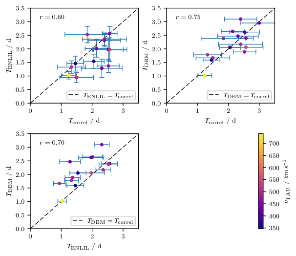
In Figure 10 (upper left panel), we compare the travel times calculated by the ENLIL model with the ones obtained from the in situ data in this work. Both travel times are also listed in Tables 2 and 3. For many events, ENLIL seems to predict a slightly faster propagation. Results for faster ICMEs (e.g. the 2012-11-28 ICME at STEREO B — ICME 6 in Tables 2 and 3) seem to agree quite well, while the slower events show larger differences. This might be the result of slower ICMEs being exposed to the disturbances in the interplanetary space for a longer time, thus accumulating a larger amount of possible uncertainties in the model. However, a more systematic statistical study based on more events should be carried out in the future to draw a solid statement on this matter.

We also calculated the mean difference between the results

and the average absolute difference

The error given here is the standard error of the mean, not the standard deviation.

A simpler model for the propagation of ICMEs is the Drag-Based Model (DBM), described in Vršnak et al. (2013) and Žic et al. (2015). The DBM is based on the assumption that beyond a distance of approximately $20\text{\,}\mathrm{R_{\mbox{$\odot$}}}$, the dominating influence on ICMEs is an “aerodynamic” drag force with an empirically determined drag parameter $\Gamma$. The main difference between DBM and ENLIL is that the former does not employ numerical MHD simulations — the drag equations can be solved analytically. Therefore, the simulation is computationally inexpensive.

Vršnak et al. (2014) already compared results from DBM and ENLIL simulations and found that the ICME arrival times at Earth predicted by the two models generally agree quite well with average absolute-value difference of below $8\text{\,}\mathrm{h}$. For these results, drag parameter values between $\Gamma=$ $0.1\text{\times}{10}^{-7}0.2\text{\times}{10}^{-7}\text{\,}{\mathrm{km}}^{-1}$ and solar wind speeds between $w=$ $400500\text{\,}\mathrm{km}\text{\,}{\mathrm{s}}^{-1}$ were used as an input for the DBM.

We apply the DBM model in such a way that the propagation of ICMEs is simulated starting from $1\text{\,}\mathrm{AU}$, where the in situ measurement of the ICME is used as input, thus avoiding the uncertainty of the propagation from the Sun up to $1\text{\,}\mathrm{AU}$. As the input for DBM, we used the local ICME speed ($v_{$1\text{\,}\mathrm{AU}$}$) and the ambient solar wind speed for each event measured at ACE or STEREO as described in section 3.1. The drag parameter $\Gamma$ was chosen to be $0.1\text{\times}{10}^{-7}\text{\,}{\mathrm{km}}^{-1}$, which is a low value that is commonly used for describing the propagation of the interplanetary shock associated with an ICME. We chose this value because the shock is related to the first step of the Forbush decrease (Cane, 2000, e.g.). Assuming that the ICME propagates outward radially, the ICMEs’ half-widths and the heliospheric longitudes of their propagation directions were taken from the DONKI database entries, as previously done for the ENLIL model (as such information is not available at $1\text{\,}\mathrm{AU}$).

The arrival times at Mars predicted by DBM are marked in Figure 2 as well as Figures 11 to 15 in the appendix. Additionally, Figure 10 (upper right panel) compares the travel times predicted by DBM to the results of the correlation method and the lower left panel compares the two models, ENLIL and DBM.

The mean difference and mean absolute difference between the results are:

On average, DBM gives slightly better results than ENLIL for these events, even though the amount of variance is similar. Probably, this is primarily due to the fact that we could use DBM for propagation from $1\text{\,}\mathrm{AU}$ to Mars instead of from the Sun.

The agreement between the DBM and ENLIL models is similar to the one of ENLIL and the correlation method results with an average absolute-value difference slightly above the value of $8\text{\,}\mathrm{h}$ determined by Vršnak et al. (2014) for the propagation up to $1\text{\,}\mathrm{AU}$. This difference seems reasonable as the propagation from the Sun out to Mars ($\sim$1.5\text{\,}\mathrm{AU}$$) takes a longer time and can therefore introduce a larger amount of error.

Under the assumption that the acceleration $a$ of an ICME stays constant between the Sun and $1\text{\,}\mathrm{AU}$ and between $1\text{\,}\mathrm{AU}$ and Mars and with a simplified, one-dimensional version of DBM (disregarding the influence of the geometric shape of the ICME), we also tried to derive the actual values of the drag parameter $\Gamma$ based on the observations and our calculated $a$ values by solving the following equation (cf. Vršnak et al., 2013, Equation 1)

for $\Gamma$.

Using the average speed $v_{\text{ICME}}=(v_{\text{launch}}+v_{$1\text{\,}\mathrm{AU}$})/2$ and $a=a_{\text{Sun},$1\text{\,}\mathrm{AU}$}$ (from Table 2 we get an estimation of $\Gamma$ between the Sun and $1\text{\,}\mathrm{AU}$, which is given in Table 3. By calculating a weighted average using the inverse errors of these $\Gamma$ values, we obtain a result of $0.09\text{\times}{10}^{-7}\text{\,}{\mathrm{km}}^{-1}$, which shows that our assumption of $\Gamma=$0.1\text{\times}{10}^{-7}\text{\,}{\mathrm{km}}^{-1}$$ was reasonable. Nonetheless, we note that the variance of $\Gamma$ for different events is considerable which reflects the dynamic and variant nature of ICMEs and suggests that the approximated constant value of $\Gamma$ in DBM may result in uncertainties in the modelling procedure. The same $\Gamma$ values could also be calculated between $1\text{\,}\mathrm{AU}$ and Mars using $v_{\text{ICME}}=\overline{v}$ and $a=a_{$1\text{\,}\mathrm{AU}$,\text{Mars}}$, however, the results have propagated uncertainties that are too large to be meaningful.