Adaptive Mantel Test for Association Testing in Imaging Genetics Data

For data $(X_{i},Y_{i})\in\mathbb{R}^{p}\times\mathbb{R}^{q},i=1,\dots,n$, we consider a stochastic model with high-dimensional parameter vector of interest $\beta$. We denote the likelihood as $\mathcal{L}(\beta)$, score vector $\mathcal{U}(\beta)=\frac{\partial\log\mathcal{L}}{\partial\beta}$, and Fisher information $\mathcal{I}(\beta)=-\mathbb{E}\frac{\partial}{\partial\beta}\mathcal{U}(\beta)$. The score test statistic for testing $H_{0}:\beta=\beta_{0}$ is $S=\mathcal{U}(\beta)^{T}(\mathcal{I}(\beta))^{-1}\mathcal{U}(\beta)|_{\beta=\beta_{0}}$ (replacing any nuisance parameters by consistent estimators).

We now derive expressions for the score test of the association of $X$ and $Y$ in the fixed effects, ridge regression, and variance components models, and show that these form a single class of linear association tests indexed by the ridge penalty $\lambda\in[0,\infty]$. Throughout this paper, we assume $X$ has been column-centered to zero mean and $Y$ has been standardized to zero mean and unit variance. The score test statistics can be compactly written by considering the singular value decomposition (SVD) of $X$. Assuming $\text{rank}(X)=r\leq\min(p,n)$, the SVD is $X=UDV^{T}$, where $U$ is $n\times r$ with $U^{T}U=I_{r}$, $D$ is an $r\times r$ diagonal matrix of singular values, where $\eta_{j},j=1,\cdots,r$ are the squared singular values, and $V$ is $p\times r$, with $V^{T}V=I_{r}$. We refer to the columns of $U$ as the principal directions of $X$. It is convenient to also define $\eta_{j}=d_{j}^{2}$, which is the variance of $X$ along the $j$th principal direction, and the principal correlation vector $Z=U^{T}Y$, which is an $r\times 1$ vector with $j$th component $Z_{j}=R(Y,U_{j})$, the Pearson correlation of $Y$ with $X$ along the $j$th principal direction. When two test statistics $T_{1}$, $T_{2}$ differ by values that are fixed under permutation of the subject labels (which do not affect the permutation $P$-value), we say that $T_{1}$ is testing equivalent to $T_{2}$, written $T_{1}\asymp T_{2}$.

We next review the Mantel test (Mantel, 1967) and show that it includes the score test considered above as a special case. The classical Mantel test, using the distance matrices for two sets of features, has been shown to exhibit extremely low power in even modestly high-dimensional settings, and so how largely fallen out of use. However, the framework of the Mantel test is extremely general, and encompasses many well-known association tests, as we will show.

Let $X$ and $Y$ be as above. For $\mathcal{K}^{\textbf{X}}(\cdot,\cdot)$ a symmetric positive semi-definite kernel (or similarity) function on $\textbf{X}\times\textbf{X}$, let $K$ be the corresponding Gram matrix with $K_{ij}=\mathcal{K}^{\textbf{X}}(X_{i},X_{j})$, and let kernel $\mathcal{K}^{\textbf{Y}}$ defined on $\textbf{Y}\times\textbf{Y}$ have corresponding Gram matrix $H$. The Mantel test statistic for these kernels is defined as

Assuming observations are exchangeable, the reference distribution under the null hypothesis of no association between $\mathcal{K}^{\textbf{X}}$ measures and $\mathcal{K}^{\textbf{Y}}$ measures, can be obtained from the observed features $X$ and $Y$ by permuting the observation labels for one set of features and calculating the empirical reference distribution for $T$. Equivalently, one can hold one matrix fixed, say $H$, and simultaneously permute the rows and columns of $K$. The expected value of this test statistic under the null hypothesis is $\mathbb{E}[T(X,Y)]=\sigma^{2}_{\varepsilon}\text{tr}(K)$, which depends on the choice of $K$.

We will focus on tests with similarity measures that can be written as $\mathcal{K}_{\mathcal{W}}(X_{i},X_{j})=\langle X_{i},X_{j}\rangle_{\mathcal{W}}=X_{i}^{T}\mathcal{W}X_{j}$ for a positive semi-definite (p.s.d.) weight matrix $\mathcal{W}$, referred to as weighted Euclidean inner products. We propose three choices for $\mathcal{W}$ and the resulting Gram matrices, which we denote $K_{F},K_{V},$ and $K_{\lambda}$, that produce Mantel tests equivalent to the score tests for the fixed effects, variance components, and ridge regression models respectively. Choosing $\mathcal{W}=I_{p}$ (the $p\times p$ identity matrix) gives the standard Euclidean inner product, with Gram matrix $K_{V}=XX^{T}$. Another natural choice for weight matrix is $\mathcal{W}=(X^{T}X)^{-1}$ (assuming the inverse exists), which is the projection matrix into $\mathcal{C}(X)$, the column space of $X$. The Gram matrix is $K_{F}=X(X^{T}X)^{-1}X^{T}.$ $K_{F}$ is also recognizable as the “hat matrix” from the fixed effects model, and is related to the Mahalanobis distance. When $X^{T}X$ is not full rank, such as when $n>p$, we can replace $(X^{T}X)^{-1}$ with a generalized inverse $(X^{T}X)^{-}$, since the similarity matrix is invariant to the choice of inverse. Alternatively, as in ridge regression (Hoerl et al., 1975), we can pre-condition the weight matrix by adding a positive constant $\lambda$ to the diagonal, i.e. $\mathcal{W}=\lambda(X^{T}X+\lambda I_{p})^{-1}$, which gives Gram matrix $K_{\lambda}=\lambda X(X^{T}X+\lambda I_{p})^{-1}X^{T}.$ Letting $H=YY^{T}$, we define the Mantel test statistics $T_{V},T_{F},T_{\lambda}$ from these Gram matrices. Note that we use the same notation for the linear model score tests and corresponding Mantel tests since these tests are equivalent under a permutation testing procedure.

Since multiplying the test statistic by a term that does not depend on both $X$ and $Y$ does not affect the permutation $P$-value, it follows from the expressions for the score tests in Proposition 1 that the score tests for the fixed effects, variance components, and ridge regression models are equivalent to the Mantel test with the Mahalanobis, Euclidean, and ridge inner products respectively. Thus the linear model score test statistics have the following equivalent interpretations: (i) the weighted norm of the correlation vector $X^{T}Y$; (ii) the weighted sum of principal correlations; (iii) the correlation of similarities of subjects in X (measured by $\mathcal{K}_{\mathcal{W}}$) with the similarities of subjects in Y (measured by the Euclidean inner product).

Given the connection between fixed effects and variance components models, we now extend the preceding results to the relationship between two sets of multivariate measurements. This extension is essential for many applications, such as heritability analysis of neuroimaging-derived phenotypes. Previous results in multivariate modeling have shown that ridge regression with tuning parameters for both response and covariates can be effective for the simultaneous prediction of multiple outcome variables (Brown & Zidek, 1980; Breiman & Friedman, 1997), thus it may be useful to consider ridge kernel similarities for both feature sets in the Mantel test.

Suppose now that each subject $i$ is measured on a $q$-variate phenotype $Y_{i}$ so that $Y$ is an $n\times q$ matrix, and assume that $Y$ is column-centered, and let $X$ be a column-centered $n\times p$ covariate matrix as before. For two tuning parameters $\lambda_{X},\lambda_{Y}>0$ and Gram matrices $H_{\lambda_{Y}}=Y(Y^{T}Y+\lambda_{Y}I_{q})^{-1}Y^{T}\mbox{ , }K_{\lambda_{X}}=X(X^{T}X+\lambda_{X}I_{p})^{-1}X^{T}$, the ridge kernel Mantel test statistic is $T_{\lambda_{X},\lambda_{Y}}=\text{tr}(H_{\lambda_{Y}}K_{\lambda_{X}})$.

To understand the underlying implications of the ridge kernel similarity measure, we consider a data-augmentation definition of ridge regression. Data augmentation has been widely used to ease the computation in several problems, such as the expectation and maximization algorithms, and Gibbs or MCMC sampling (Duncan & Horn, 1972; Dempster et al., 1977; Dempster et al., 1981; Tanner & Wong, 1987; Van & Meng, 2001; Gelman et al., 2014). In particular, Hodges (1998) described how data augmentation can be used as a device to write hierarchical models in the form of linear models.

We demonstrate in A.2 that $T_{\lambda_{X},\lambda_{Y}}$ corresponds to a similar augmented data model as in the univariate response case. Examining the log-likelihood, it is apparent that $\lambda_{X}$ shrinks $B$ toward zero, $\lambda_{Y}$ encourages smaller sums of the reciprocals of the eigenvalues of $\Sigma_{\varepsilon}$. Shrinking $B$ by the ridge penalization induced by $\lambda_{X}$ is equivalent to replacing $X(X^{T}+\lambda_{X}I_{p})^{-1}X^{T}$ with $XX^{T}$ when $\lambda_{X}$ is large. When $\lambda_{Y}$ is large, we expect that $\Sigma_{\varepsilon}$ is approximately proportional to an identity matrix, that is $Y(Y^{T}Y+\lambda_{Y})^{-1}Y^{T}$ is approximately proportional to $YY^{T}$. Thus, large values of tuning parameters favors the use of Euclidean distance in that modality, which ignores the dependence structure of the features, leading to $\lim_{\lambda_{X}\to\infty,\lambda_{Y}\to\infty}T_{\lambda_{X},\lambda_{Y}}=\text{tr}(XX^{T}YY^{T})$.

Correlation metrics and the proportion of variance explained are commonly used for quantifying the strength of association of $X$ and $Y$. The product-moment (or Pearson) correlation is a symmetric measure of cosine similarity of the two random vectors, and is stated without reference to a particular model. In contrast, the proportion of variance in $Y$ explained by $X$ is necessarily measured with respect to some model stated with $Y$ as response and $X$ as explanatory variables, and is thus not a symmetric measure. Correlation is simple to calculate, but can only measure the linear relationship of $X$ and $Y$, and may be misleading if $X$ and $Y$ have a significant nonlinear relationship. Measuring variance explained instead requires the selection and fitting of a model, allowing one to specify the functional relationship of $X$ and $Y$ to be measured. We here develop relationships between these measures and the Mantel test statistics defined in the previous section.

The sample (Pearson) correlation of the similarity measures of all subjects can be naturally defined as

The quantities $R(K,H)$ and $\text{tr}(K,H)$ are related to known statistics for many choices of $K$ and $H$. For example, $R(K_{F},H_{F})$ is proportional to Hooper’s trace correlation $R_{T}^{2}$ (Hooper, 1959), which is defined as $R_{T}^{2}=\frac{1}{q}\text{tr}\left((Y^{T}Y)^{-1}Y^{T}X(X^{T}X)^{-1}X^{T}Y)\right)=\sqrt{\frac{p}{q}}R(K_{F},H_{F})$. This is also proportional to the trace of the canonical correlation matrix, and thus the test $T_{F,F}=\text{tr}(K_{F}H_{F})$ can be interpreted as testing the sum of the squared canonical correlations.

The statistic $T_{F,V}=\text{tr}(X(X^{T}X)^{-1}X^{T}YY^{T})$ for multivariate $X$ and $Y$ can be interpreted similar to the univariate case. Defining the principal correlations $Z_{jk}=U_{j}^{T}Y_{k}$, which is the correlation of the $k$th feature of $Y$ along the $j$th principal direction of $X$. Writing $T_{F,V}=\text{tr}(K_{F}H_{V})=\sum_{j=1}^{r}\sum_{k=1}^{s}Z_{jk}^{2}$, this statistic can be understood as testing the Frobenius norm of the matrix of principal correlations. Proposition 2 shows that the sample correlation of similarities for the three choices of $K$ above can be conveniently related through the singular value decomposition (SVD) of $X$ and the principal correlation vector.

The proportion of variance explained in both fixed-effect and random-effect models can be expressed as functions of Mantel statistics. In the genetics literature, $h^{2}$ is known as the additive, or narrow-sense, genetic heritability (Yang et al., 2011; Liu et al., 2007), defined as the proportion of phenotypic variance explained by additive SNP effects. Moment based estimators for $h^{2}$ have been proposed, such as the Haseman-Elston estimator , which regress pairwise distances in phenotypes to pairwise genetic correlation of related subjects (Haseman & Elston, 1972; Elston et al., 2000). This has recently been adapted to unrelated subjects (Yang et al., 2010; Golan et al., 2014), and extended to multivariate phenotypes as well (Ge et al., 2016).

To define heritability of multivariate phenotypes, we consider the variance components model with multivariate response $Y\sim N(0,\Sigma_{A}\otimes G+\Sigma_{E}\otimes I_{n})$, where $\Sigma_{A}$ is the genetic covariance of the features of $Y$, $G=XX^{T}/p$, and $\Sigma_{E}$ is the covariance of the subject errors. The proportion of variance explained by this model is defined as

In the simplified case of uncorrelated phenotypes with homogeneous genetic effect $\sigma^{2}$ and uncorrelated subjects with constant error variance $\sigma^{2}_{\varepsilon}$, the covariance matrices are $\Sigma_{A}=\sigma^{2}I_{q}$ and $\Sigma_{E}=\sigma^{2}_{\varepsilon}$. In this case, the heritability reduces to $h^{2}=\sigma^{2}/(\sigma^{2}+\sigma^{2}_{\varepsilon})$. The univariate variance components model (Equation 3) is then recovered when $q=1$. The following proposition connects the correlation of Gram matrices with the proportion of variance explained in the multivariate variance components model.

Effectively using kernel methods requires an appropriate selection of the kernel function and tuning parameters for the particular setting. Selection methods have been extensively considered in the context of prediction problems, with cross-validation as the de facto standard. Cross-validation is a straight-forward and practical selection method for prediction, but may be difficult to implement for hypothesis testing, since the type I error rate needs to be controlled. Furthermore, the tuning parameter selected by minimizing the CV MSE may not necessarily yield the highest powered test. In this section, we develop the adaptive Mantel test (AdaMant), a novel extension of the classical MT to utilize the ridge kernel in association testing methods. By using the maximum $P$-value from a set of $T_{\lambda}$ statistics, AdaMant is able to simultaneously test across a set of tuning parameters and kernels without the need to directly apply adjustments for multiple tests. In comparison to the RV-test, which relies on a single metric, AdaMant tests across a set of metrics, and can therefore achieve higher power in certain settings, as shown by the simulations in Section 5.

The “adaptive” procedure used here is similar to the adaptive sum of powered score test algorithm described in Xu et al. (2017). The procedure receives as input a list of pairs of metrics/kernels $\{(\mathcal{K}^{\textbf{X}}_{m},\mathcal{K}^{\textbf{Y}}_{m})|m=1,\cdots M\}$ from which the matrices $K_{m}=\mathcal{K}^{\textbf{X}}_{m}(X)$ and $H_{m}=\mathcal{K}^{\textbf{Y}}_{m}(Y)$ are computed for each metric pair, $m=1,\cdots,M$. These metrics may be from a single family with varying tuning parameters, such as ridge kernels with different penalization terms, or may include kernels from different families.

For each $m=1,\cdots,M$, $P_{m}$ is calculated as the $P$-value of the Mantel test with metrics $\mathcal{K}_{m}^{\textbf{X}}$ and $\mathcal{K}_{m}^{\textbf{Y}}$ for $X$ and $Y$ respectively. The AdaMant test statistic is defined as the minimum of these values,

A permutation procedure is practical for calculating the reference distribution for $P^{(0)}$. For each $m$, and $b=1,\cdots,B$, $H_{m}^{(b)}$ is generated by permuting rows and columns of $H$ simultaneously, and the corresponding test statistic $P^{(b)}$ is calculated. The AdaMant $P$-value is then calculated as

Let us now illustrate the utility of AdaMant through an example varying the relationship of the PCs of $X$ with $Y$ generated from a variance components model. Suppose that $X$ is a $100\times 2$ matrix of covariates drawn iid from a standard normal distribution, and $Y\sim N(0,\sigma^{2}K^{(\theta)}+\sigma^{2}_{\varepsilon})$, with $K^{(\theta)}=U\Theta\Delta^{2}\Theta^{T}U^{T}$ for $\Theta$ the $2\times 2$ rotation matrix for angle $\theta$. Figure 2 shows the results of applying AdaMant with weights for the Euclidean, Mahalanobis, and ridge kernels ($\lambda=10$) for data generated with $\theta=0,0.12\pi,0.3\pi$. In each case, AdaMant selects the weighting that most emphasizes the empirical direction of association of $X$ and $Y$. This clearly demonstrates the potential advantage of AdaMant if the direction of association of $X$ and $Y$ is different than the first PC of $X$. In this case, AdaMant will likely be a more powerful test than methods such as the RV test, which corresponds to using only the Euclidean weighting.

If the feature space is very high-dimensional or if $n$ is large, a straightforward implementation of Algorithm 1 may be computationally impractical. However, when only ridge kernels with varying values of $\lambda$ are included in AdaMant, there are two approaches that can be used to greatly reduce the computational cost.

The first approach utilizes the SVD $X=UDV^{T}$. The computational complexity needed for finding the SVD for $X$ is $O(np^{2})$. Once the SVD is computed, we can compute $Z=U^{T}Y$ and $S_{\lambda}=\sum_{i=1}^{r}\frac{\eta_{i}}{\lambda+\eta_{i}}Z_{i}^{2}$, which has a total complexity of $O(nr)$. Note that when $p\gg n$, the rank $r$ is often the same as $n$; as a result, the cost needed for calculating $S_{\lambda}$ is $O(nr)=O(n^{2})$. Calculating the test statistics for $B$ permutations requires $O(Bn^{2})$, for a total computational complexity of $O(np^{2}+Bn^{2})$.

Alternatively, when $p$ is very large relative to $n$, we can use the identity $X(X^{T}X+\lambda I)^{-1}=(XX^{T}+\lambda I)^{-1}X,$ so that the dimension of the matrix to be inverted is lowered to $n\times n$, rather than $p\times p$. From this identity, $K_{\lambda}$ can be rewritten as $K_{\lambda}=(XX^{T}+\lambda I_{n})^{-1}XX^{T}.$ Note that calculating $K_{\lambda}$ involves multiplying the $n\times p$ matrix $X$ and the $p\times n$ matrix $X^{T}$, multiplying two $n\times n$ matrices, and inverting an $n\times n$ matrix. When $p\gg n$, the computation cost is dominated by calculating $XX^{T}$, which has a complexity of $O(n^{2}p)$. The Mantel test statistic can be calculated as

which has a complexity of $O(n^{2})$. With $B$ permutations, the total computational complexity is $O(n^{2}p+Bn^{2})$, which is less than the required computational complexity using SVD. Thus, switching from the feature space to the subject space (i.e., from a $p\times p$ similarity matrix of the features to an $n\times n$ similarity matrix of the subjects), has a computational advantage.

A main advantage of AdaMant is to allow for simultaneous testing over a set of tuning parameter values while incurring substantially less loss of power compared to multiple testing adjustment methods such as Bonferroni. Although it does not impose an overly conservative adjustment for multiple testing, the power of AdaMant does decrease as the number of metrics considered increases. Conversely, the test results are highly sensitive to the choice of parameters to test, thus one must take some care in the selection of the included parameters, balancing the desire to use a wide range of parameter values, with the gains of using a small set of parameters. When only ridge kernels are included in AdaMant, previous results on the role of the ridge penalty term in predictive modeling can help with the identification of a reasonable set of values to test.

Specifically, it has been shown that when the ridge penalty $\lambda$ is chosen to be the noise-to-signal ratio $\sigma_{\varepsilon}^{2}/\sigma^{2}=(1-h^{2})/h^{2}$, the resulting shrinkage estimator $\hat{\beta}_{\lambda}$ is identical to the best linear unbiased predictor (BLUP) for the random effects model, and moreover, for a new observation with unknown response the predictions using the ridge with and random effects models are the same for $\lambda=\sigma_{\varepsilon}^{2}/\sigma^{2}$ (Campos et al., 2013). Consequently, a reasonable set of penalty terms can usually be determined in practice by positing a priori a likely range for the noise to signal ratio or a related quantity such as the proportion of variance explained.

The scientific interpretation and range of plausible values of $h^{2}$ will depend on the specific modalities of $X$ and $Y$. For instance, a genome-wide heritability of $h^{2}>0.5$ is very high (and would likely have already been discovered by previous studies), whereas a heritability of $h^{2}<0.1$ is probably not scientifically interesting. As a point of reference, most estimated heritability in the UK Biobank data is between 0.1 to 0.4 (Ge et al., 2017).

To assess the performance of AdaMant for univariate phenotypes, the simulated response $Y$ was generated from either the variance components model (Eq. 10) or the fixed effects model (Eq. 9), with $n=200$ observations, number of covariates $p$ ranging from 100 to 500, and $\sigma^{2}_{e}=1$ fixed. The design matrix $X$ was generated from $n$ draws from a $p$-variate normal distribution $N(0,\Sigma_{X})$, where $\Sigma_{X}$ is chosen to have a compound symmetric structure with $\rho=0.1$. AdaMant was applied using the adamant R-package (Pluta, 2018) with $H=YY^{T}$ and $K_{\lambda}$ for $\lambda\in\{100,10^{3},2.5\times 10^{3},5\times 10^{3},7.5\times 10^{3},10^{4},2.5\times 10^{4},\infty\}$ (where $\infty$ corresponds to the Euclidean inner product similarity measure), with 500 permutations. For each setting, 500 simulations were run. Figure 3 shows the simulation results for data generated from the variance components model with $\sigma^{2}_{b}=0.035^{2}$, and the fixed effects model with $\beta_{j}=(-1)^{j}0.05,j=1,\dots,p$.

The simulation results indicate that the power of AdaMant is competitive with the best of the single-parameter MT for the values considered. For the variance components setting, $\lambda=1000$ exhibited the highest power for the ridge MT. As anticipated, the power of the ridge MT exhibits unimodal behavior, such that the power increases to its peak for $\lambda=1000$, and decreases as $\lambda\to\infty$. We note that even though the variance components model is the true data generating mechanism, the test power is substantially increased over the variance components score test through the use of the ridge kernels.

When the response data is generated from the fixed effects model, the simulation results show that using a penalized ridge kernel produces much higher power than competing tests, with $\lambda=100$ giving the highest power across all values of $p$. These results suggest that the variance components test is severely underpowered when the relationship of $X$ and $Y$ is strongest along principal components of $X$ with low variance. Moreover, the RV coefficient, dCov, and aSPC tests perform equally poorly in this setting.

Additional simulation results for sparse effects (setting the effect size of some features of $X$ to zero) are provided in the online supplement A.4.

Since we are primarily interested in applying AdaMant to imaging genetics data, we also consider the test performance on simulated data with structure similar to realistic EEG and SNP data (see Figure 4). To generate the genetic data, observations were placed into one of two balanced groups to form two groups of genetically similar observations. For group $k,k=1,2$, a group-wide SNP vector $X^{(k)}$ of length 300 is generated by iid sampling from a discrete uniform distribution over $\{-1,0,1\}$; for subject $i$ in group $k$, a subject-specfic error vector $\varepsilon^{(k)}_{i}\sim N(0,I_{300})$ are added to the group SNP vector to get the subject SNP vector $X^{(k)}_{i}=X^{(k)}+\varepsilon^{(k)}_{i}$.

To generate data with spectral characteristics similar to real EEG data, for each observation 20 time series of length 1000 were generated (for 20 “channels”) as a weighted mixture of two independent AR(2) processes with spectral peaks at 5.12 Hz and 12.8 Hz and second-order AR-coefficient fixed at -1, resulting in a time series with two peaks at the chosen frequencies, with the magnitude of the peaks determined by the mixing weights. The mixing weights for a random selection of 10 of the channels (common across all subjects) are drawn iid from $N(0,1)$, so that no genetic effect exists for these channels. To link the genetic features to the remaining channels, the $200\times 10\times 2$ array $W$ of AR(2) mixing weights was generated from a multivariate variance components model, such that for channel $j$ and AR(2) basis $m$, the subject weight vector is generated from $W_{jm}\sim N(0,\sigma^{2}_{g}YY^{T})$, where $\sigma^{2}_{g}$ is varied across simulations to control the strength of genetic association. The pair of weights for each subject and channel are then each squared and divided so that the weights sum to one. From the resulting EEG data, the connectivity matrix for each observation is calculated from either the pairwise coherence for all pairs of channels.

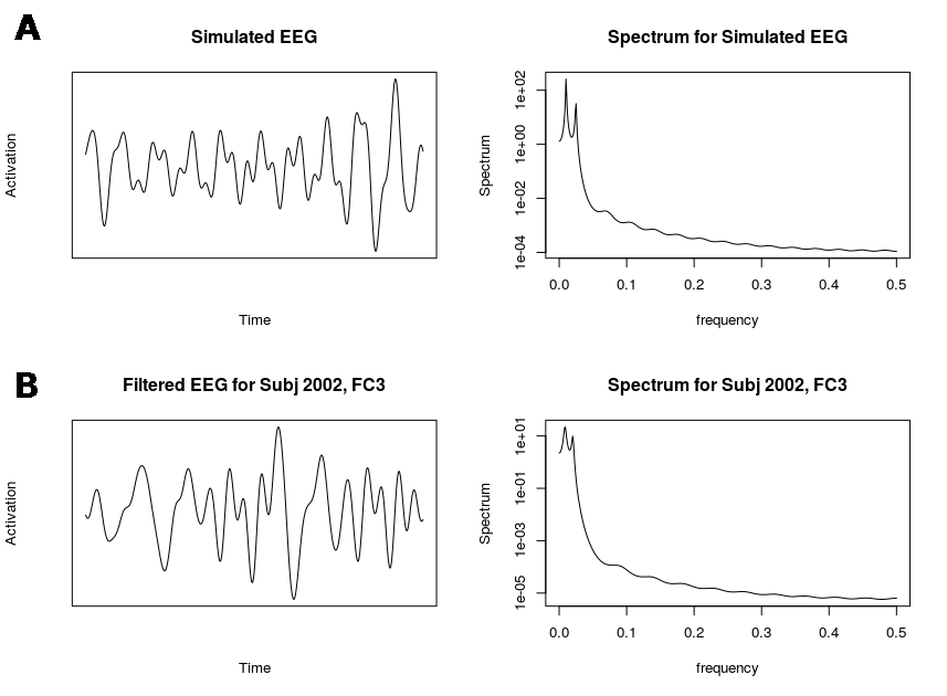
In applying AdaMant, similarity of observations in the EEG domain is then computed from the ridge kernel applied to the vectorized upper triangles of the observations’ theta coherence matrices (resulting in 190 features), with candidate penalty terms $\Lambda_{Y}\in\{10,100,\infty\}$. Similarity in the genetics domain is computed from the ridge kernel applied to the observations’ SNP vectors, with candidate penalty terms $\Lambda_{X}=\{10,100,\infty\}$. 500 simulations were run for effect sizes equal to $\sigma=\{0,2.5\times 10^{-6},5\times 10^{-6},7.5\times 10^{-6},1\times 10^{-5}\}$. The simulation results show (Figure 5) that AdaMant again has power competitive with other association testing methods in this setting.

We next consider data from 350 healthy college students from Beijing Normal University (BNU) who participated in a visual working memory task conducted by our co-author, during which 64-channel EEG was recorded at 1 kHz. These data are part of a broader set of imaging, genetics, and behavioral data collected with the goal of identifying neurological features of brain connectivity (measured via EEG) that are significantly associated with both genetic features and cognitive performance. In the present study, we focus on testing the association of EEG coherence with a set of genome-wide SNPs, a set of candidate SNPs identified in a meta-analysis of educational attainment (EA), and a set of candidate SNPs previously implicated as potential factors in Alzheimer’s Disease (AD).

The coherence of two signals is a measure of the oscillatory correspondence (or spectral similarity) of two signals within a specified frequency band. An outline of computing the coherence of two time series using the discrete Fourier transform is given in A.5.1; a more comprehensive treatment is provided in Shumway & Stoffer (2011), and Ombao & Van (2008). EEG coherence has been implicated in many cognitive processes and neurological diseases, for instance, in associative learning (Fiecas & Ombao, 2016), as a predictor of ability in certain linguistic and visuo-spatial tasks (Kang et al., 2017), and in Alzheimer’s disease (Engels et al., 2015; Vecchio et al., 2018) and schizophrenia (Griesmayr et al., 2014).

The experimental task is depicted in Figure 6. Subjects were asked to remember the positioning of the red bars (the targets) on the left or right side of the image as indicated by the arrow in the center of the image. Six experimental conditions were used for 2, 3, 4, 6, and 8 targets, and for 2 targets + 2 blue distractors. Each trial consists of the presentation of four images in sequence, with a total duration approximately three seconds, structured as follows: (i) fixation image for $400\pm 200$ ms; (ii) the standard array to be memorized (100 ms); (iii) the blank maintenance image (900 ms); (iv) comparison array is shown, and subjects are prompted to respond within 2000 ms if the targets in the comparison array match or mismatch the standard array. The total duration of the experiment was 5-10 minutes for each subject. EEG data was downsampled to 256 Hz, channels with corrupted signals removed, and a band pass filter from 1 – 40 Hz was applied. Independent components analysis was then used to remove physiological artifacts such as eyeblinks and other muscle movement (Delorme & Makeig, 2004; Makeig et al., 2004). Lastly, all subjects were manually inspected to remove any remaining artifacts. The coherence between two EEG channels at a particular frequency $\omega$ is a measure of the oscillatory concordance of the the two signals at $\omega$. Details of calculating the coherence are given in A.5.1. The pairwise coherence for $q$ EEG channels is a $q\times q$ symmetric matrix, from which we extract the upper triangle and vectorize to form the $n\times\genfrac{(}{)}{0.0pt}{}{q}{2}$ matrix $Y$.

Channel topography and coordinates are available from the BioSemi website (BioSemi, 2015). For our analysis, we consider coherence restricted to the 25 most anterior channels (“Frontal”), and fronto-parietal (FP) coherence from 30 channels covering the frontal and parietal lobes. This results in 300 distinct features for the 25 frontal channels, and 435 features for the fronto-parietal channels. Figure 10 shows the location of the channels for the frontal and fronto-parietal groups.

Genotype data from approximately $5\times 10^{5}$ single nucleotide polymorphisms (SNPs) for all subjects was measured, of which 484496 autosomal SNPs meeting quality control thresholds ($MAF>1\%,HWE<0.001$) were included for heritability testing. Data processing and heritability testing was conducted with PLINK v1.90b4.4 and GCTA 1.91.5 beta2. Let $X$ be the column-standardized SNP data matrix.

To determine whether the heritability of EEG coherence in the theta, alpha, and beta bands is significantly greater than zero, AdaMant was performed with $K=XX^{T}$ (which is proportional to the usual genetic relationship matrix), $H=Y(Y^{T}Y+\lambda I)^{-1}Y^{T}$ for $\lambda\in\{10,100,1000,\infty\}$, using 5000 permutations.

The most significantly heritable coherence was found to be the theta band (4 – 8 Hz) for the frontal channels, with $P=0.0458$. Other bands tested were not found to be significantly heritable, additional results can be found in Table 1. The estimated mean heritability of theta coherence for the frontal channels is $\hat{h}^{2}=0.165$, although there is large variance in this estimate due to the somewhat small sample size.

Following the scientific aims of the BNU imaging genetics study, it is of interest to determine whether genetic markers linked to educational attainment (EA) are significantly associated with EEG coherence during the visual working memory experiment. SNPs were selected from the meta-analysis of educational attainment by Okbay et al. (2016), which identified over $3\times 10^{5}$ SNPs found to be significantly associated with EA at a level of 0.01. These SNPs were also found to show significantly elevated expression specifically in developing neural tissue, thus it is plausible they may be significantly associated with other aspects of cognitive development and performance.

Testing the association of the top 100 EA SNPs with EEG coherence, we found that similarities from beta and gamma band coherence are significantly associated with genetic similarity measured from the top 100 SNPs from the EA gene set for the Frontal and Fronto-parietal coherence. The beta band was the most significantly associated, with $P=0.0104$ for the frontal channels and $P=0.013$ for the FP channels.

For a more targeted test of genetic influence on EEG coherence, a group of 11 SNPs that have been identified as potentially related to Alzheimer’s Disease were selected in order to determine if these SNPs are related to working memory brain function in healthy individuals. AdaMant test was performed with $\lambda\in\{0.5,1,5,10,100,1000,\infty\}$ for ridge kernel similarity of the coherence data, and using 5000 permutations. Genetic similarity of subjects was calculated as the $L_{2}$ inner product of the standardized SNP data for all tests. For the alpha band, AdaMant $P$-values were $P=0.065$ and $P=0.381$ for all channels and frontal channels respectively. Results for the theta band were $P=0.416$ and $P=0.085$ for all 64 channels and frontal channels respectively. Since the adaptive Mantel test was used, these $P$-values already take into account testing across multiple $\lambda$. In the case of the alpha band, the test results suggest that coherence involving channels outside of the selected frontal channels may be associated with genetic similarity determined by the 11 AD SNPs, whereas for the theta band, the SNP association appears stronger when considering only the frontal channels.

Additional results on the specific channels and SNPs that are most associated, and discussion of the scientific relevance is provided in the online supplement A.5.3.

References

- Afonja (1972) Biyi Afonja “The moments of the maximum of correlated normal and t-variates” In Journal of the Royal Statistical Society. Series B (Methodological) JSTOR, 1972, pp. 251–262
- Bertolino et al. (2006) Alessandro Bertolino et al. “Additive Effects of Genetic Variation in Dopamine Regulating Genes on Working Memory Cortical Activity in Human Brain” In Journal of Neuroscience 26.15 Society for Neuroscience, 2006, pp. 3918–3922
- BioSemi (2015) BioSemi In BioSemi Instrumentation, 2015 URL: https://www.biosemi.com/headcap.htm
- Breiman & Friedman (1997) Leo Breiman and Jerome Friedman “Predicting multivariate responses in multiple linear regression” In Journal of the Royal Statistical Society: Series B (Statistical Methodology) 59.1 Wiley Online Library, 1997, pp. 3–54
- Brown & Zidek (1980) Philip Brown and James Zidek “Adaptive multivariate ridge regression” In The Annals of Statistics JSTOR, 1980, pp. 64–74
- Campos et al. (2013) Gustavo de Campos et al. “Prediction of complex human traits using the genomic best linear unbiased predictor” In PLoS genetics 9.7 Public Library of Science, 2013, pp. e1003608
- Chen et al. (2012) Lu Chen et al. “Polymorphisms of CR1, CLU and PICALM confer susceptibility of Alzheimer’s disease in a southern Chinese population” In Neurobiology of aging 33.1 Elsevier, 2012, pp. 210–e1
- Delorme & Makeig (2004) Arnaud Delorme and Scott Makeig “EEGLAB: an open source toolbox for analysis of single-trial EEG dynamics including independent component analysis” In Journal of neuroscience methods 134.1 Elsevier, 2004, pp. 9–21
- Dempster et al. (1977) Arthur Dempster, Nan Laird and Donald Rubin “Maximum likelihood from incomplete data via the EM algorithm” In Journal of the royal statistical society. Series B (methodological) JSTOR, 1977, pp. 1–38
- Dempster et al. (1981) Arthur Dempster, Donald Rubin and Robert Tsutakawa “Estimation in covariance components models” In Journal of the American Statistical Association 76.374 Taylor & Francis, 1981, pp. 341–353
- Duncan & Horn (1972) David Duncan and Susan Horn “Linear dynamic recursive estimation from the viewpoint of regression analysis” In Journal of the American Statistical Association 67.340 Taylor & Francis, 1972, pp. 815–821
- Elston et al. (2000) Robert Elston, Sarah Buxbaum, Kevin Jacobs and Jane Olson “Haseman and Elston revisited” In Genetic epidemiology 19.1, 2000, pp. 1–17
- Engels et al. (2015) Marjolein Engels et al. “Declining functional connectivity and changing hub locations in Alzheimer’s disease: an EEG study” In BMC neurology 15.1 BioMed Central, 2015, pp. 145
- Fiecas & Ombao (2016) Mark Fiecas and Hernando Ombao “Modeling the evolution of dynamic brain processes during an associative learning experiment” In Journal of the American Statistical Association 111.516 Taylor & Francis, 2016, pp. 1440–1453
- Ge et al. (2017) Tian Ge et al. “Phenome-wide heritability analysis of the UK Biobank” In PLoS genetics 13.4 Public Library of Science, 2017, pp. e1006711
- Ge et al. (2016) Tian Ge et al. “Multidimensional heritability analysis of neuroanatomical shape” In Nature communications 7 Nature Publishing Group, 2016, pp. 13291
- Gelman et al. (2014) Andrew Gelman et al. “Bayesian data analysis” CRC press Boca Raton, FL, 2014
- Goeman et al. (2004) Jelle Goeman, Sara Van, Floor De and Hans Van “A global test for groups of genes: testing association with a clinical outcome” In Bioinformatics 20.1 Oxford University Press, 2004, pp. 93–99
- Goeman et al. (2006) Jelle Goeman, Sara Van and Hans Van “Testing against a high dimensional alternative” In Journal of the Royal Statistical Society: Series B (Statistical Methodology) 68.3 Wiley Online Library, 2006, pp. 477–493
- Golan et al. (2014) David Golan, Eric Lander and Saharon Rosset “Measuring missing heritability: inferring the contribution of common variants” In Proceedings of the National Academy of Sciences 111.49 National Acad Sciences, 2014, pp. E5272–E5281
- Griesmayr et al. (2014) Birgit Griesmayr et al. “EEG theta phase coupling during executive control of visual working memory investigated in individuals with schizophrenia and in healthy controls” In Cognitive, Affective, & Behavioral Neuroscience 14.4 Springer, 2014, pp. 1340–1355
- Harold et al. (2009) Denise Harold et al. “Genome-wide association study identifies variants at CLU and PICALM associated with Alzheimer’s disease” In Nature genetics 41.10 Nature Publishing Group, 2009, pp. 1088
- Haseman & Elston (1972) JK Haseman and RC Elston “The investigation of linkage between a quantitative trait and a marker locus” In Behavior genetics 2.1 Springer, 1972, pp. 3–19
- Hodges (1998) James Hodges “Some algebra and geometry for hierarchical models, applied to diagnostics” In Journal of the Royal Statistical Society: Series B (Statistical Methodology) 60.3 Wiley Online Library, 1998, pp. 497–536
- Hoerl et al. (1975) Arthur Hoerl, Robert Kannard and Kent Baldwin “Ridge regression: some simulations” In Communications in Statistics-Theory and Methods 4.2 Taylor & Francis, 1975, pp. 105–123
- Hooper (1959) John Hooper “Simultaneous equations and canonical correlation theory” In Econometrica: Journal of the Econometric Society JSTOR, 1959, pp. 245–256
- Kang et al. (2017) Jun-Su Kang, Amitash Ojha, Giyoung Lee and Minho Lee “Difference in brain activation patterns of individuals with high and low intelligence in linguistic and visuo-spatial tasks: An EEG study” In Intelligence 61 Elsevier, 2017, pp. 47–55
- Kwee et al. (2008) Lydia Kwee et al. “A powerful and flexible multilocus association test for quantitative traits” In The American Journal of Human Genetics 82.2 Elsevier, 2008, pp. 386–397
- Laird & Ware (1982) Nan Laird and James Ware “Random-effects models for longitudinal data” In Biometrics JSTOR, 1982, pp. 963–974
- Liu et al. (2007) Dawei Liu, Xihong Lin and Debashis Ghosh “Semiparametric Regression of Multidimensional Genetic Pathway Data: Least-Squares Kernel Machines and Linear Mixed Models” In Biometrics 63.4 Wiley Online Library, 2007, pp. 1079–1088
- Liu et al. (2013) Guiyou Liu et al. “Lack of association between PICALM rs3851179 polymorphism and Alzheimer’s disease in Chinese population and APOE4-negative subgroup” In Neurobiology of aging 34.4 Elsevier, 2013, pp. 1310–e9
- Liu & Lin (2018) Zhonghua Liu and Xihong Lin “A Geometric Perspective on the Power of Principal Component Association Tests in Multiple Phenotype Studies” In Journal of the American Statistical Association Taylor & Francis, 2018, pp. 1–36
- Makeig et al. (2004) Scott Makeig, Stefan Debener, Julie Onton and Arnaud Delorme “Mining event-related brain dynamics” In Trends in cognitive sciences 8.5 Elsevier, 2004, pp. 204–210
- Mantel (1967) Nathan Mantel “The detection of disease clustering and a generalized regression approach” In Cancer research 27.2 Part 1 AACR, 1967, pp. 209–220
- Nadarajah & Kotz (2008) Saralees Nadarajah and Samuel Kotz “Exact distribution of the max/min of two Gaussian random variables” In IEEE Transactions on very large scale integration (VLSI) systems 16.2 IEEE, 2008, pp. 210–212
- Okbay et al. (2016) Aysu Okbay et al. “Genome-wide association study identifies 74 loci associated with educational attainment” In Nature 533.7604 Nature Publishing Group, 2016, pp. 539
- Ombao & Van (2008) Hernando Ombao and S“’ebastien Van “Evolutionary coherence of nonstationary signals” In IEEE Transactions on Signal Processing 56.6 IEEE, 2008, pp. 2259–2266
- Omelka & Hudecov“’a (2013) Marek Omelka and S“’arka Hudecov“’a “A comparison of the Mantel test with a generalised distance covariance test” In Environmetrics 24.7 Wiley Online Library, 2013, pp. 449–460
- Onton et al. (2005) Julie Onton, Arnaud Delorme and Scott Makeig “Frontal midline EEG dynamics during working memory” In Neuroimage 27.2 Elsevier, 2005, pp. 341–356
- Pan (2011) Wei Pan “Relationship between genomic distance-based regression and kernel machine regression for multi-marker association testing” In Genetic epidemiology 35.4 Wiley Online Library, 2011, pp. 211–216
- Pluta (2018) Dustin Pluta “AdaMant R-Package” In GitHub, 2018 DOI: https://doi.org/10.5281/zenodo.2025858
- Robert & Escoufier (1976) Paul Robert and Yves Escoufier “A unifying tool for linear multivariate statistical methods: the RV-coefficient” In Applied statistics JSTOR, 1976, pp. 257–265
- Salem et al. (2010) Rany Salem, Daniel O’Connor and Nicholas Schork “Curve-based multivariate distance matrix regression analysis: application to genetic association analyses involving repeated measures” In Physiological genomics 42.2 American Physiological Society Bethesda, MD, 2010, pp. 236–247
- Satterthwaite (1946) Franklin Satterthwaite “An approximate distribution of estimates of variance components” In Biometrics bulletin 2.6 JSTOR, 1946, pp. 110–114
- Sauseng et al. (2005) Paul Sauseng, Wolfgang Klimesch, Manuel Schabus and Michael Doppelmayr “Fronto-parietal EEG coherence in theta and upper alpha reflect central executive functions of working memory” In International Journal of Psychophysiology 57.2 Elsevier, 2005, pp. 97–103
- Schaid (2010) Daniel Schaid “Genomic similarity and kernel methods I: advancements by building on mathematical and statistical foundations” In Human heredity 70.2 Karger Publishers, 2010, pp. 109–131
- Schork & Zapala (2012) Nicholas Schork and Matthew Zapala “Statistical properties of multivariate distance matrix regression for high-dimensional data analysis” In Frontiers in genetics 3 Frontiers, 2012, pp. 190
- Shumway & Stoffer (2011) Robert Shumway and David Stoffer “Time series regression and exploratory data analysis” In Time series analysis and its applications Springer, 2011
- Simons & Spiers (2003) Jon Simons and Hugo Spiers “Prefrontal and medial temporal lobe interactions in long-term memory” In Nature reviews neuroscience 4.8, 2003, pp. 637–648
- Sz“’ekely et al. (2007) G“’abor Sz“’ekely, Maria Rizzo and Nail Bakirov “Measuring and testing dependence by correlation of distances” In The annals of statistics 35.6 Institute of Mathematical Statistics, 2007, pp. 2769–2794
- Tanner & Wong (1987) Martin Tanner and Wing Wong “The calculation of posterior distributions by data augmentation” In Journal of the American statistical Association 82.398 Taylor & Francis Group, 1987, pp. 528–540
- Tzeng et al. (2009) Jung-Ying Tzeng et al. “Gene-Trait Similarity Regression for Multimarker-Based Association Analysis” In Biometrics 65.3 Wiley Online Library, 2009, pp. 822–832
- Van & Meng (2001) David Van and Xiao-Li Meng “The art of data augmentation” In Journal of Computational and Graphical Statistics 10.1 Taylor & Francis, 2001, pp. 1–50
- Vecchio et al. (2018) Fabrizio Vecchio et al. “Sustainable method for Alzheimer dementia prediction in mild cognitive impairment: Electroencephalographic connectivity and graph theory combined with apolipoprotein E” In Annals of neurology 84.2 Wiley Online Library, 2018, pp. 302–314
- Vogler et al. (2014) C Vogler et al. “Substantial SNP-based heritability estimates for working memory performance” In Translational psychiatry 4.9 Nature Publishing Group, 2014, pp. e438
- Wessel & Schork (2006) Jennifer Wessel and Nicholas Schork “Generalized genomic distance–based regression methodology for multilocus association analysis” In The American Journal of Human Genetics 79.5 Elsevier, 2006, pp. 792–806
- Xu et al. (2017) Zhiyuan Xu, Gongjun Xu and Wei Pan “Adaptive testing for association between two random vectors in moderate to high dimensions” In Genetic Epidemiology Wiley Online Library, 2017
- Yang et al. (2010) Jian Yang et al. “Common SNPs explain a large proportion of the heritability for human height” In Nature genetics 42.7 Nature Publishing Group, 2010, pp. 565
- Yang et al. (2011) Jian Yang, S Lee, Michael Goddard and Peter Visscher “GCTA: a tool for genome-wide complex trait analysis” In The American Journal of Human Genetics 88.1 Elsevier, 2011, pp. 76–82
- Zhang (2005) Jin-Ting Zhang “Approximate and asymptotic distributions of chi-squared–type mixtures with applications” In Journal of the American Statistical Association 100.469 Taylor & Francis, 2005, pp. 273–285
- Zhou et al. (2010) Yi Zhou et al. “Association analysis between the rs11136000 single nucleotide polymorphism in clusterin gene, rs3851179 single nucleotide polymorphism in clathrin assembly lymphoid myeloid protein gene and the patients with schizophrenia in the Chinese population” In DNA and cell biology 29.12 Mary Ann Liebert, Inc. 140 Huguenot Street, 3rd Floor New Rochelle, NY 10801 USA, 2010, pp. 745–751
Appendix A APPENDIX
A.1 Proofs of Propositions
A.1.1 Proposition 1
Let be a column-centered matrix with , SVD , and squared singular values . Let be an response vector, where is an semi-positive definite covariance matrix that depends on . Define , the vector of principal correlations, and define , and by Equations 1, 2, and 4.
- 1.
Connections between linear model score tests. The score tests for the fixed effects, variance components, and ridge regression models form a single class of tests parameterized by the ridge tuning parameter . is testing equivalent to the variance components score test as , Assuming , is testing equivalent to the fixed effects score statistic, .
- 2.
Score test reference distributions. Let be iid chi-squared random variables with one degree of freedom. Let be a chi-squared random variable with degrees of freedom.
- (a)
- (b)
- (c)
Proof
Under the null hypothesis of , the reference distribution is . Since each is iid standard normal, for iid copies of a chi-squared random variable with one degree of freedom.
A.1.2 Proposition 2
Let be an column centered matrix of covariates with and singular value decomposition , with singular values . For convenience, we define . Suppose be an response vector, and let and . Assume that is standardized so that and .
Fixed Effects
For simplicity, here we assume . Note that when is not full rank, one can replace with and the similarity matrix is invariant to the choice of a generalized inverse.
Random Effects
- 3.
Ridge Regression
(1) The matrix is the standard projection matrix (the “hat matrix”) from linear regression, giving the identity The result follows directly from the definition of and
If we replace with its singular value decomposition, we have
(2) In a random-effect linear model, the variance-covariance structure of the outcome vector is a function of the similarity that is defined using the dot product: . Let . We have
(3) In a ridge regression, let and . We have
Let , we have
The correlation coefficient based on the similarity matrices is
(4) When , we assume that . The result follows immediately.
When , let and express the correlation at in terms of :
Using L’Hospital’s rule, it is not difficult to see that
i.e.,
Note that ; in other words, the ridge regression method shrinks the correlation. Another observation is that when , has orthogonal columns and all the correlations are identical.
A.1.3 Proposition 3
Assume is an column-standardized, full row-rank matrix (which requires ), and assume is a -variate column-standardized random vector. Define Gram matrices and (for which and under the above assumptions).
The method of moments estimator is
The expectation of the correlation of Gram matrices is
First compute following standard results on the quadratic forms.
Plugging in and solving for gives the desired method of moments estimator
Corollary In the setting of Proposition 3, with a univariate vector () and for fixed , , and , with , the expected correlation is a function of , with maximum and minimum dependent on the noise-to-signal ratio .
For , the expected correlation is bounded by
with upper and lower bounds attained by and respectively.
with upper and lower bounds attained at and respectively.
Define the function . Here can be interpreted as a candidate value for . The derivative of is
It follows that gives . The signs of the derivative can be checked to show that this is in fact a minimum of . The maximum and minimum of attained on (the range of determined by ) depends on the relationship of to the range of , for which there are three cases.
When , is in the range of , and so the minimum of is attained here. Since is strictly increasing for , the maximum of is attained at .
with upper and lower bounds attained by and , respectively.
When , is strictly increasing in the range of , so the maximum and minimum are attained are the right and left endpoints of the interval, respectively.
When , is strictly decreasing in the range of , so the maximum and minimum are attained at the left and right endpoints of the interval, respectively.
A.2 Multivariate Ridge
Previous results have shown that ridge regression with tuning parameters for both and can be effective for the simultaneous prediction of multiple outcome variables (Brown & Zidek, 1980; Breiman & Friedman, 1997), thus it may be useful to consider ridge kernel similarities for both and . For two tuning parameters and Gram matrices , the ridge kernel Mantel test statistic is . The corresponding augmented data model is