Imperfect Thermalizations Allow for Optimal Thermodynamic Processes

The maximum extractable work of $\rho_{\rm S}^{(0)}$ is given by the change of (non-equilibrium) free energy between initial and final state [36, 37]

$\displaystyle\Delta F\equiv F(\rho_{\rm S}^{(0)},H_{\rm S})-F(\tau_{\rm S},H_{\rm S}),$

(13)

where $F(\rho,H)=\Tr(\rho H)-TS(\rho)$, with $S(\rho)$ the von Neumann entropy $S(\rho)=-\Tr[\rho\ln\rho]$ and

$\displaystyle\tau_{\rm S}:=\frac{e^{-\beta H_{\rm S}}}{\Tr[e^{-\beta H_{\rm S}}]}.$

(14)

Note that $\Delta F$ in (13) is the difference between initial and final free energy (and not vice versa), which is convenient for our sign convention in which $W>0$ when work is extracted from the system.

Following Refs. [31, 14], we now briefly discuss an explicit protocol leading to (13). In order to construct an optimal process, the excitation probabilities $\{q_{k}\}_{k=0}^{N}$ are chosen to start at $q_{0}=p_{0}$ and increase strictly monotic to $q_{N}=e^{-\beta\epsilon_{\rm S}}/(1+e^{-\beta\epsilon_{\rm S}})$. Hence, $\tau_{\rm B}^{(0)}=\rho_{\rm S}^{(0)}$ and in the case of maximal work extraction $\tau_{\rm B}^{(N)}=\tau_{\rm S}$. The total process is described by the following unitary operation on SBW,

$\displaystyle U=\prod_{k=1}^{N}U^{(k)}_{\rm SBW}$

(15)

where each $U^{(k)}_{\rm SBW}$ acts on S, W and the $k^{\rm th}$ bath qubit, see Figure 1. Using the short hand notation, $\ket{a,b,c}:=\ket{a}_{\rm S}\otimes\ket{b}_{\rm B}\otimes\ket{c}_{\rm W}$ and $\omega_{k}:=E_{k}-\epsilon_{\rm S}$, $U^{(k)}_{\rm SBW}$ takes the form

$\displaystyle\begin{split}U^{(k)}_{\rm SBW}=\int_{x}&dx\bigg(\ket{0,1,x}\bra{1,0,x+\omega_{k}}+h.c.\\ &+\ket{0,0,x}\bra{0,0,x}+\ket{1,1,x}\bra{1,1,x}\bigg)\end{split}$

(16)

Let us also write this expression in matrix form using the basis $\{\ket{0,0,x},\ket{0,1,x},\ket{1,0,x+\omega_{k}},\ket{1,1,x}\}$

$\displaystyle U^{(k)}_{\rm SBW}$

$\displaystyle=\int_{x}dx\begin{pmatrix}1&0&0&0\\ 0&0&1&0\\ 0&1&0&0\\ 0&0&0&1\end{pmatrix}_{x},$

(17)

where the subscript $x$ indicates that the basis depends on $x$. The action of $U^{(k)}_{\rm SBW}$ is illustrated in Figure 2. Note that

• •

  $U^{(k)}_{\rm SBW}$ acts upon a degenerate energy subspace, and hence condition 1., as given by (12), is satisfied. It is straightforward to see that condition 2. is satisfied as well.

• •

  At the global level, the final state after applying $U^{(k)}_{\rm SBW}$ becomes correlated. At the level of the reduced states, it leads to a swap between the states $\rho_{\rm S}\leftrightarrow\tau^{(k)}_{\rm B}$,

• •

  As $k$ increases, the state of S progressively changes from $\rho_{\rm S}^{(0)}$ to $\tau_{\rm S}$, which mimics an isothermal process.

Furthermore, the total extracted work $W=\Tr\left(H_{\rm W}(U\rho^{(0)}U^{\dagger}-\rho^{(0)})\right)$ from (15) satisfies,

$\displaystyle W=\Delta F-\mathcal{O}(1/N),$

(18)

hence becoming maximal in the limit $N\rightarrow\infty$ (see e.g. [31, 14]).

Let us now describe the set of imperfect operations we consider. For clarity, we start by presenting a simple model to describe lack of control on the operations $U_{\rm SBW}^{(k)}$. For that, note that the unitary (16) can be implemented by turning on the interaction $g\sigma_{x}$ in the subspace $\ket{0,1,x}$, $\ket{1,0,x+\omega_{x}}$ for a time $\pi\hbar/2g$. If the timing is not precise, the corresponding unitary $\tilde{U}^{(k)}_{\rm SBW}$ takes the form,

$\displaystyle\tilde{U}^{(k)}_{\rm SBW}$

$\displaystyle=\int dx\begin{pmatrix}1&0&0&0\\ 0&\sqrt{\alpha_{k}}&i\sqrt{1-\alpha_{k}}&0\\ 0&i\sqrt{1-\alpha_{k}}&\sqrt{\alpha_{k}}&0\\ 0&0&0&1\end{pmatrix},$

(19)

where $\alpha_{k}\in[0,1]$ quantifies the error in the $k^{\rm th}$ step: for $\alpha_{k}=0$ we apply the desired full rotation and for $\alpha_{k}=1$ we do nothing on the state. After (19), the reduced states of S and B, given by $\rho_{\rm S/B}^{(k)}=\Tr_{\rm BW/SW}\left(\tilde{U}^{(k)}_{\rm SBW}\rho^{(k)}\tilde{U}^{(k){\dagger}}_{\rm SBW}\right)$, take the form

$\displaystyle\begin{split}\rho^{(k)}_{\rm S}&=\alpha_{k}\rho^{(k-1)}_{\rm S}+(1-\alpha_{k})\tau_{\rm B}^{(k)}\\ \rho_{\rm B}^{(k)}&=\alpha_{k}\tau_{\rm B}^{(k)}+(1-\alpha_{k})\rho^{(k-1)}_{\rm S}.\end{split}$

(20)

Hence, here the lack of control essentially leads to a partial thermalization process.

In fact, there are more general processes that lead to (20). In Appendix A, we consider arbitrary thermal operations [5] on the relevant degenerate subspaces $\ket{0,1,x}$, $\ket{1,0,x+\omega_{x}}$. By this, we aim to model the situation where the relevant subspace where the experimentalist is acting upon is not thermally isolated, e.g., there is decoherence in the unitary operations being implemented. We then show that all operations of this form lead to the same model of noise (20), with the $\alpha_{k}$’s being complex functions of the applied specific thermal operation. Therefore, we conclude that (20) is generally valid when we restrict ourselves to the operations described above which map states from the degenerate energy subspaces $\ket{0,1,x}$, $\ket{1,0,x+\omega_{x}}$ to states on that same subspace while acting arbitrarily on an auxiliary system. This is the model we will consider for the rest of our work. As a remark, note that (20) naturally allows for generalizations when considering systems beyond qubits.

Before moving further, it is important to keep in mind that the set of imperfect operations we described is of course not the most general noisy, or thermal, operation. The motivation behind our choice is that, as we will now show, thermodynamic processes can still be constructed despite the lack of control. Conversely, if we lift the restrictions made above, it is not difficult to convince oneself that other types of noise, e.g., thermal noise acting on S or W only, are detrimental for thermodynamic purposes and cannot be compensated for. This is discussed in Appendix B.

We first show that it is possible to obtain $W\rightarrow\Delta F$ for any $\alpha<1$ in the limit of $N\rightarrow\infty$. For clarity of the presentation, we find it convenient to present here the case where $\rho_{\rm S}=|0\rangle\langle 0|_{\rm S}$ and $\epsilon_{\rm S}=0$ and discuss the general case for arbitrary initial states of S and higher dimensional systems in Section 2.2.3 and Appendix D. Note that the case $\rho_{\rm S}=|0\rangle\langle 0|_{\rm S}$ and $\epsilon_{\rm S}=0$ corresponds to well-known information to energy conversion, where $\Delta F=k_{B}T\ln 2$ work can be extracted from one bit of information. The opposite direction, resetting one bit of information while investing work $\Delta F=k_{B}T\ln 2$, the so-called erasure, works analogously since we are looking at reversible processes.

To compute the average energy gain of the weight W, we first notice that the work extracted in step $k$ is

	$\displaystyle W^{(k)}$	$\displaystyle=\Tr\hskip-1.42262pt\left[\big(\rho_{\rm W}^{(k)}-\rho_{\rm W}^{(k-1)}\big)H_{\rm W}\right]$
		$\displaystyle=\Tr\hskip-1.42262pt\left[H_{\rm B}^{(k)}\!\left(\tau_{\rm B}^{(k)}\!-\!\rho_{\rm B}^{(k)}\right)\!-\!H_{\rm S}\!\left(\rho_{\rm S}^{(k)}\!-\!\rho_{\rm S}^{(k-1)}\right)\right]\!,$		(27)

which follows from energy conservation. Thus, the total average work extracted after $N$ steps is the sum

	$\displaystyle W$	$\displaystyle=\sum_{k=1}^{N}\!\Tr\!\left[H_{\rm B}^{(k)}\!\left(\tau_{\rm B}^{(k)}\!-\!\rho_{\rm B}^{(k)}\right)\!-\!H_{\rm S}\!\left(\rho_{\rm S}^{(k)}\!-\!\rho_{\rm S}^{(k-1)}\right)\right]$
		$\displaystyle=(1\!-\!\alpha)\sum_{k=1}^{N}\Tr\left[\left(H_{\rm B}^{(k)}\!-\!H_{\rm S}\right)\left(\tau_{\rm B}^{(k)}\!-\!\rho_{\rm S}^{(k-1)}\right)\right]\!.$		(28)

For the qubit case, we have

$\displaystyle W$

$\displaystyle=(1-\alpha)\sum_{k=1}^{N}(E_{k}-\epsilon_{\rm S})(q_{k}-p_{k-1}).$

(29)

Let us now use our choice of initial conditions $\epsilon_{\rm S}=0$ and $p_{0}=0$, i.e., initially $\rho_{\rm S}=\ket{0}\bra{0}_{\rm S}$. The distribution of bath qubits is taken to be

$\displaystyle q_{k}=\frac{k}{2N}\quad\Rightarrow\quad\Delta q_{k}:=q_{k}-q_{k-1}=\frac{1}{2N}\ \ \forall k,$

(30)

so that $\tau_{\rm B}^{(0)}=\rho_{\rm S}$ and $\tau_{\rm B}^{(N)}=\tau_{\rm S}$. Note that this specific distribution is chosen here for simplicity and to give an explicit upper bound – we later discuss more general settings. Using (26), we get an explicit form for the excitation probabilities of $\rho_{\rm S}^{(k)}$,

$\displaystyle p_{k}$

$\displaystyle=(1-\alpha)\sum_{i=1}^{k}\alpha^{k-i}\frac{i}{2N}=q_{k}-\frac{\alpha(1-\alpha^{k})}{1-\alpha}\Delta q_{k},$

(31)

where we can already see that they only differ by $\mathcal{O}\left(1/N\right)$ compared to the excitation probabilities $q_{k}$ we would get using error-free unitaries. That is, for large $N$ our state $\rho_{S}$ is at every step close to the corresponding thermal state, and hence it follows approximately the isothermal trajectory of the state transformation. We now show that for large $N$ this also happens at an optimal work cost, i.e., that the work extracted becomes arbitrary close to the one in the error-free case. Using (31), the average extracted work simplifies to

	$\displaystyle W$	$\displaystyle=(1-\alpha)\sum_{k=1}^{N}E_{k}\left(q_{k}-p_{k-1}\right)$
		$\displaystyle=(1-\alpha)\sum_{k=1}^{N}E_{k}\left(q_{k}-q_{k-1}+\frac{\alpha-\alpha^{k}}{1-\alpha}\Delta q_{k}\right)$
		$\displaystyle=\sum_{k=1}^{N}E_{k}\Delta q_{k}(1-\alpha^{k})$
		$\displaystyle=\Delta F-\frac{\Gamma}{N}-\varepsilon-\mathcal{O}\left(\frac{1}{N^{2}}\right),$		(32)

where $\Delta F-\frac{\Gamma}{N}-\mathcal{O}\left(\frac{1}{N^{2}}\right)$ with $\Gamma=\mathcal{O}\left(E_{\rm max}\right)$ is the maximum average work that can be extracted with $N$ steps in the error-free protocol, i.e., with $\alpha=0$. The loss due to the noise characterized by $\alpha$ is described by $\varepsilon=\frac{\alpha}{1-\alpha}\frac{\Lambda}{N}+\mathcal{O}\left(\frac{1}{N^{2}}\right)$ and corresponds to the difference between the work extracted in the optimal protocol ($\alpha=0$) and the one with faulty unitaries $(\alpha\neq 0$). It can be upper bounded by

	$\displaystyle\varepsilon$	$\displaystyle=\frac{1}{2N}\sum_{k=1}^{N}E_{k}\alpha^{k}=\frac{k_{B}T}{2N}\sum_{k=1}^{N}\ln\left(\frac{2N-k}{k}\right)\alpha^{k}$
		$\displaystyle<\frac{k_{B}T}{2N}\sum_{k=1}^{N}\ln\left(2N\right)\alpha^{k}<\frac{\alpha}{1-\alpha}\frac{k_{B}T\ln(2N)}{2N},$		(33)

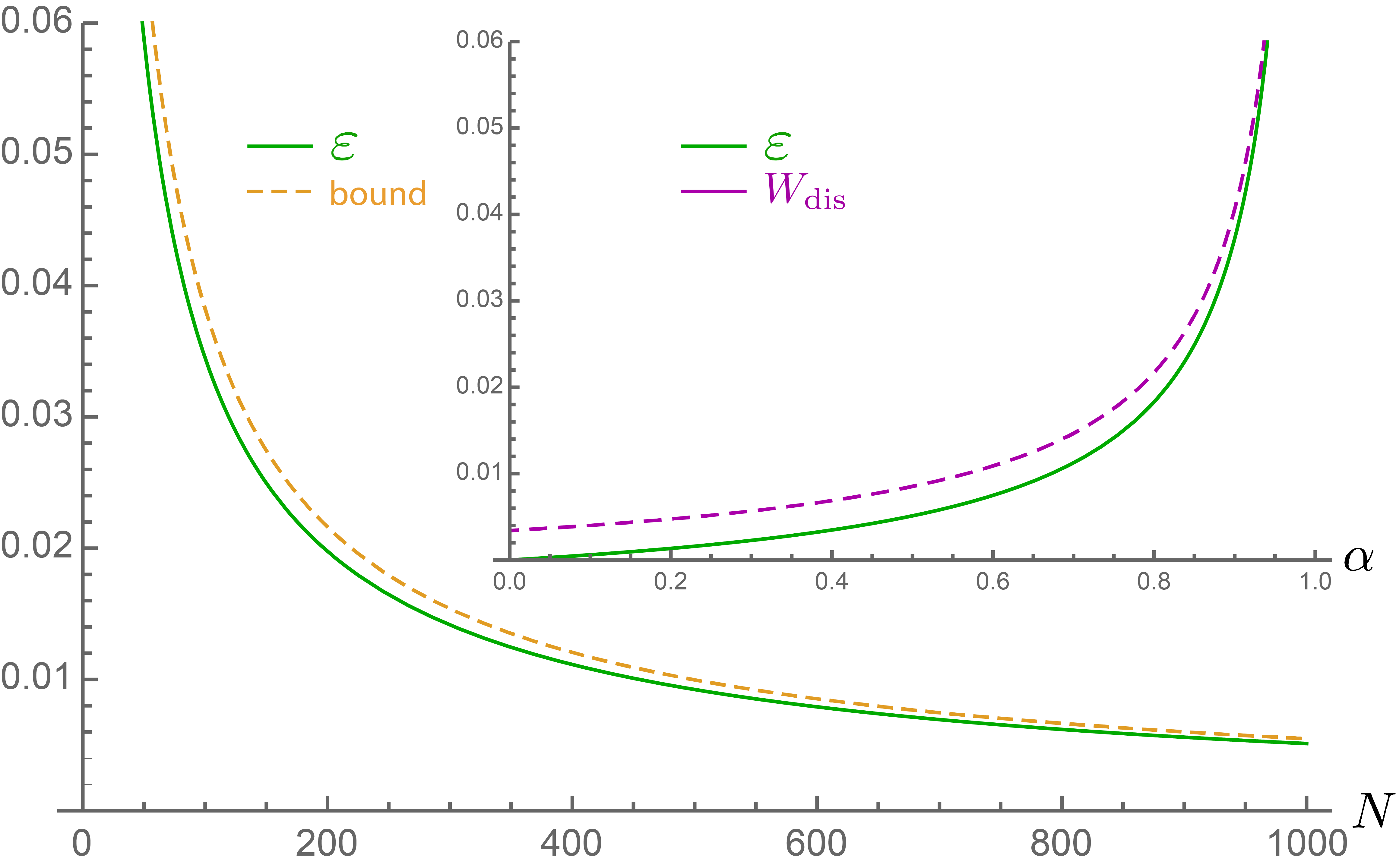
which implies $\Lambda=\mathcal{O}\left(E_{\rm max}\right)$. In the limit $N\rightarrow\infty$, we get $\varepsilon\rightarrow 0$ and hence $W\rightarrow\Delta F$ for any $\alpha<1$. In Figure 3 we plot the numerical value of loss $\varepsilon$ and the upper bound (33). We observe that the deviation is small and the bound almost tight. We also plot $\varepsilon$ together with the total dissipation $W_{\rm dis}=\Delta F-W$ for finitely many steps as a function of $\alpha$.

The fluctuations of work are captured by the probability distribution $P(w)=\bra{w}\rho_{\rm W}\ket{w}$, where $\rho_{\rm W}$ is the final state of W, $\rho_{\rm W}=\Tr_{\rm SB}U\rho^{(0)}U^{\dagger}$ and $\rho^{(0)}$ is defined in (7). That is, the work fluctuations are mapped to energy fluctuations of the weight, which initially starts in a well-defined energy ¹¹ 1 Note that, since we consider non-coherent states of S, the same fluctuations would be obtained by using the more standard two-energy-measurement scheme on SB together [38]. The two approaches are equivalent here. .

In Appendix C, a lengthy calculation shows that for $\rho_{\rm S}=|0\rangle\langle 0|_{\rm S}$, $\epsilon_{\rm S}=0$, $\alpha_{k}\leq\alpha<1\ \forall k$ and distribution (30), the variance of $P(w)$ decreases as $\mathcal{O}\left(\ln(N)/N\right)$, and hence disappears in the limit $N\rightarrow\infty$. This result implies that an amount $k_{B}T\ln 2$ of work can be extracted with certainty from one bit of information, even when dealing with partial thermalizations as in (24). The work probability distribution of this process is illustrated in Figure 4.

Given this result, the case of $\rho_{\rm S}=(1-p_{0})|0\rangle\langle 0|_{\rm S}+p_{0}|1\rangle\langle 1|_{\rm S}$ and $\epsilon_{\rm S}\neq 0$ can be easily understood qualitatively. First of all, recall that for general $\rho_{\rm S}$ the optimal protocol is such that $H_{\rm B}^{(0)}$ satisfies $\tau_{\rm B}^{(0)}=\rho_{\rm S}$ and $H_{\rm B}^{(N)}=H_{\rm S}$. Secondly, since $P(w)$ is linear in $\rho_{\rm S}$, we can write $P(w)=(1-p_{0})P_{0}(w)+p_{0}P_{1}(w)$ where $P_{0,1}(w)$ is the probability distribution starting the protocol with $|0\rangle\langle 0|_{\rm S}$ and $|1\rangle\langle 1|_{\rm S}$, respectively. From our previous result, it follows that $P_{0}(w)$ tends to a peaked distribution, which is now centered at $w_{0}=F(\rho_{\rm S},H_{\rm B}^{(0)})-F(\tau_{\rm S},H_{\rm S})$ (recall that we consider the protocol for maximal work extraction from $\rho_{\rm S}$). Similarly, $P_{1}(w)$ tends also to a peaked distribution centered at $w_{1}=\epsilon_{\rm S}-E_{0}+F(\rho_{\rm S},H_{\rm B}^{(0)})-F(\tau_{\rm S},H_{\rm S})$. Putting everything together, and noting that $w_{0}=k_{B}T\ln((1-p_{0})/(1-p_{\rm S}^{(eq)}))$ and $w_{1}=k_{B}T\ln(p_{0}/p_{\rm S}^{(eq)})$, we can write the work probability distribution in the limit $N\rightarrow\infty$ as

	$\displaystyle P(w)$	$\displaystyle\stackrel{{\scriptstyle N\rightarrow\infty}}{{\longrightarrow}}p_{0}\delta\left(w-k_{B}T\ln\frac{p_{0}}{\ p_{\rm S}^{(eq)}}\right)$
		$\displaystyle+(1-p_{0})\delta\hskip-2.84526pt\left(w-k_{B}T\ln\frac{1-p_{0}}{\ 1-p_{\rm S}^{(eq)}}\right)$		(34)

where $\delta(w-x)$ is the Delta function. Crucially, this distribution is independent of $\alpha$, and hence we recover previous results where perfect thermalization operations ($\alpha=0$) were assumed [14, 20].

Although our results have been derived for qubit systems, they can be naturally extended to qudits. For that we consider the model of partial thermalizations (24). This implies for $\rho_{\rm S}^{(k)}$ in (25) that (assuming $\rho_{\rm S}^{(0)}=\tau_{\rm B}^{(0)}$)

	$\displaystyle\rho_{\rm S}^{(k)}$	$\displaystyle=(1-\alpha)\sum_{j=0}^{k}\alpha^{j}\tau^{(k-j)}_{\rm B}+\alpha^{k}\tau_{\rm B}^{(0)}$
		$\displaystyle=\tau_{\rm B}^{(k)}\!-\!(1\!-\!\alpha)\sum_{j=0}^{k}\alpha^{j}(\tau^{(k)}_{\rm B}\!-\!\tau^{(k-j)}_{\rm B})\!+\!\mathcal{O}(\alpha^{k}).$		(35)

Let us define the continuously differentiable family of Hamiltonians $H(s)$ for $s\in[0,1]$, such that we can draw $H_{\rm B}^{(k)}:=H(k/N)$, and similarly the family of states $\tau(s)$ for $s\in[0,1]$, such that $\tau_{B}^{(j)}=\tau(j/N)$ and $\dot{\tau}(s)\equiv\frac{d}{ds}\tau(s)$. We can then expand $\tau^{(k)}_{\rm B}-\tau^{(k-j)}_{\rm B}$ over $1/N$ in (35) to obtain,

	$\displaystyle\rho_{\rm S}^{(k)}$	$\displaystyle=\tau_{\rm B}^{(k)}-(1-\alpha)\sum_{j=0}^{k}\frac{j}{N}\alpha^{j}\dot{\tau}(k/N)+\mathcal{O}(1/N^{2})$
		$\displaystyle\approx\tau_{\rm B}^{(k)}-\frac{\alpha}{N(1-\alpha)}\dot{\tau}(k/N)+\mathcal{O}(1/N^{2})$		(36)

Hence, we see how the factor $\alpha/(1-\alpha)N$ in (2) naturally arises under imperfect thermalizations. It is a consequence of the state $\rho_{S}^{(k)}$ lagging behind the thermal state $\tau^{(k)}_{\rm B}$.

In general, computing the average extracted work is more involved as it depends both on $\tau_{\rm B}^{(k)}$ and the Hamiltonians $H_{\rm B}^{(k)}$. This is done in Appendix D by using the continuous expansion described above. In particular, it is convenient to introduce the continuous limit of the non-equilibrium free energy function,

$\displaystyle F(s):=F(\tau(s),H_{\rm S})$

(37)

with $s\in[0,1]$. In Appendix D, we show (in the case of a full-rank initial state) that $W_{\rm dis}\equiv\Delta F-W$ satisfies at order $1/N$

	$\displaystyle W_{\rm dis}=$	$\displaystyle-\frac{1}{2N}\left(1+\frac{2\alpha}{1-\alpha}\right)\int_{0}^{1}\hskip-4.2679ptds\hskip 2.84526pt\Tr(\dot{H}(s)\dot{\tau}(s))$
		$\displaystyle+\frac{\alpha}{N(1-\alpha)}\left(\dot{F}(1)-2\dot{F}(0_{+})\right).$		(38)

The minus sign in the first term arises, since

$\displaystyle\int_{0}^{1}\hskip-4.2679ptds\hskip 2.84526pt\Tr(\dot{H}(s)\dot{\tau}(s))\leq 0$

(39)

for any trajectory of Hamiltonians $H(s)$, which, for example, can be seen using the techniques of Refs. [39, 40]. The second contribution to the dissipation takes place only at the extremes of the trajectory, when S is put in contact with B for the first/last time. In particular, it is worth noticing that if $\tau(1)=e^{-\beta H_{\rm S}}/\mathcal{Z}_{S}$, then we have that $\dot{F}(1)=0$ because $F(s)$ is minimized when the state is thermal. By taking an appropriate trajectory, we can also guarantee $\dot{F}(0)=0$. The more interesting contribution is the first term, which depends on the whole trajectory $H(s)$. Crucially, the dependence on $\alpha$ of the error is independent of the trajectory and is always given by an overall factor $\alpha/(1-\alpha)$. An important consequence of (38) is that protocols that minimize dissipation for $\alpha=0$ (see [40] for examples) will also minimize dissipation for imperfect thermalizations.

In the above discussion we assumed $\rho_{\rm S}^{(0)}=\tau_{\rm B}^{(0)}$. This is always possible to fulfill if $\rho_{\rm S}^{(0)}$ has full rank. If this condition is not fulfilled, one obtains an additional error term in the dissipated work, which is detailled in Appendix D. Let us here discuss the limit of optimal protocols. For any $\delta>0$ it is possible to choose $H(s)$ such that $\lVert\tau_{\rm B}^{(0)}-\rho_{\rm S}^{(0)}\rVert_{1}\leq\delta\ll 1$. In this case, one finds that the additional error term scales as $\mathcal{O}\left(\delta\log(1/\delta)\right)$ and similarly

$\displaystyle-\int_{0}^{1}\hskip-4.2679ptds\hskip 2.84526pt\Tr(\dot{H}(s)\dot{\tau}(s))=\mathcal{O}\left(\log(1/\delta)\right).$

(40)

If we now choose $\delta=\mathcal{O}\left(1/N\right)$ we thus recover the scaling behaviour

$\displaystyle W_{\rm dis}=\mathcal{O}\left(\frac{\log N}{N}\right),$

(41)

in accordance with our explicit calculation for the qubit example.

Let us also briefly comment on our assumption that the $\alpha_{k}$ in (20) are random variables with identical expectation value $\alpha$, which is independent of $N$. This assumption is in fact not crucial for the main results –although it is very convenient for the computations–, the reason being that our result holds for any $\alpha<1$. Note that we can always decrease the individual values $\alpha_{k}$ without compromising the work extraction protocol. As a consequence, even if the expectation value of the $\alpha_{k}$ would change with $k$, one can guarantee convergence to an optimal thermodynamic process as long as $\alpha_{k}\leq\alpha<1,\forall k$. Furthermore, even if $\alpha=1-C/N$ for some constant $C>0$, one still obtains the optimal expected work in the limit $N\rightarrow\infty$ (also see section 3). Similarly, we strongly expect that our results also hold for typical realizations of the $\alpha_{k}$, provided that each $\alpha_{k}$ is chosen independently with expectation values bounded away from $1$. Indeed, we expect that our results still hold even if a diverging number of $\alpha_{k}$ is equal to $1$ provided that these $\alpha_{k}$ are a vanishing fraction of all the $\alpha_{k}$ in the limit $N\rightarrow\infty$.

It is worth pointing out that even when dealing with qubits, there exist uncontrolled interactions that are thermodynamically detrimental and cannot be compensated for. For example, letting S simply thermalize with B without raising the energy in W can only decrease the extractable work. Similarly, if B and W exchange energy, W may lose energy to the bath. In order to build an optimal thermodynamic process, it is needed that B continuously thermalizes S (and not W) while W is extracting work from it. A more detailed description of interactions that cannot be tolerated can be found in Appendix B.

Finally, it is important to realize that, although we have focused our attention on optimal work extraction, our results also allow for optimal state transformations in the other direction, i.e., they can be used for converting a thermal state to a given final state at optimal work cost. More generally, they apply to the interconversion of any two states at minimal work cost. Furthermore, we note that although our results have been derived for a particular model within the resource theory of thermodynamics, we expect that similar results can be obtained in other frameworks, such as [41, 15, 13, 20, 42]. One such example is illustrated in the next section.

References

• [1] John Goold, Marcus Huber, Arnau Riera, Lídia del Rio, and Paul Skrzypczyk. The role of quantum information in thermodynamics—a topical review. Journal of Physics A: Mathematical and Theoretical, 49(14):143001, Feb 2016. ISSN 1751-8121. doi: 10.1088/1751-8113/49/14/143001. URL http://dx.doi.org/10.1088/1751-8113/49/14/143001.
• [2] Sai Vinjanampathy and Janet Anders. Quantum thermodynamics. Contemporary Physics, 57(4):545–579, Jul 2016. ISSN 1366-5812. doi: 10.1080/00107514.2016.1201896. URL http://dx.doi.org/10.1080/00107514.2016.1201896.
• [3] H.-P Breuer and Francesco Petruccione. The Theory of Open Quantum Systems. Oxford University Press, 01 2006. doi: 10.1093/acprof:oso/9780199213900.001.0001.
• [4] Märio Ziman, Peter Štelmachovič, and Vladimír Bužek. Description of quantum dynamics of open systems based on collision-like models. Open Systems & Information Dynamics, 12(1):81–91, Mar 2005. ISSN 1573-1324. doi: 10.1007/s11080-005-0488-0. URL https://doi.org/10.1007/s11080-005-0488-0.
• [5] Fernando G. S. L. Brandão, Michał Horodecki, Jonathan Oppenheim, Joseph M. Renes, and Robert W. Spekkens. Resource theory of quantum states out of thermal equilibrium. Phys. Rev. Lett., 111:250404, Dec 2013. doi: 10.1103/PhysRevLett.111.250404. URL https://link.aps.org/doi/10.1103/PhysRevLett.111.250404.
• [6] H. Wilming, R. Gallego, and J. Eisert. Second law of thermodynamics under control restrictions. Phys. Rev. E, 93:042126, Apr 2016. doi: 10.1103/PhysRevE.93.042126. URL https://link.aps.org/doi/10.1103/PhysRevE.93.042126.
• [7] J Lekscha, H Wilming, J Eisert, and R Gallego. Quantum thermodynamics with local control. Physical Review E, 97(2):022142, 2018. doi: 10.1103/PhysRevE.97.022142.
• [8] Eric G Brown, Nicolai Friis, and Marcus Huber. Passivity and practical work extraction using gaussian operations. New Journal of Physics, 18(11):113028, 2016. doi: 10.1088/1367-2630/18/11/113028. URL http://stacks.iop.org/1367-2630/18/i=11/a=113028.
• [9] Nicolai Friis and Marcus Huber. Precision and work fluctuations in gaussian battery charging. Quantum, 2:61, apr 2018. doi: 10.22331/q-2018-04-23-61.
• [10] Matteo Lostaglio, Álvaro M Alhambra, and Christopher Perry. Elementary thermal operations. Quantum, 2:52, 2018. doi: 10.22331/q-2018-02-08-52.
• [11] Christopher Perry, Piotr Ćwikliński, Janet Anders, Michał Horodecki, and Jonathan Oppenheim. A sufficient set of experimentally implementable thermal operations for small systems. Phys. Rev. X, 8:041049, Dec 2018. doi: 10.1103/PhysRevX.8.041049. URL https://link.aps.org/doi/10.1103/PhysRevX.8.041049.
• [12] J. Nulton, P. Salamon, B. Andresen, and Qi Anmin. Quasistatic processes as step equilibrations. The Journal of Chemical Physics, 83(1):334–338, jul 1985. doi: 10.1063/1.449774. URL https://doi.org/10.1063/1.449774.
• [13] Janet Anders and Vittorio Giovannetti. Thermodynamics of discrete quantum processes. New Journal of Physics, 15(3):033022, mar 2013. doi: 10.1088/1367-2630/15/3/033022. URL https://doi.org/10.1088%2F1367-2630%2F15%2F3%2F033022.
• [14] P. Skrzypczyk, A. J. Short, and S. Popescu. Extracting work from quantum systems. arXiv:1302.2811, 2013. URL https://arxiv.org/abs/1302.2811.
• [15] David Reeb and Michael M Wolf. An improved landauer principle with finite-size corrections. New Journal of Physics, 16(10):103011, oct 2014. doi: 10.1088/1367-2630/16/10/103011. URL https://doi.org/10.1088%2F1367-2630%2F16%2F10%2F103011.
• [16] Valerio Scarani, Mário Ziman, Peter Štelmachovič, Nicolas Gisin, and Vladimír Bužek. Thermalizing quantum machines: Dissipation and entanglement. Phys. Rev. Lett., 88:097905, Feb 2002. doi: 10.1103/PhysRevLett.88.097905. URL https://link.aps.org/doi/10.1103/PhysRevLett.88.097905.
• [17] P. Filipowicz, J. Javanainen, and P. Meystre. Theory of a microscopic maser. Phys. Rev. A, 34:3077–3087, Oct 1986. doi: 10.1103/PhysRevA.34.3077. URL https://link.aps.org/doi/10.1103/PhysRevA.34.3077.
• [18] Carlton M. Caves and G. J. Milburn. Quantum-mechanical model for continuous position measurements. Phys. Rev. A, 36:5543–5555, Dec 1987. doi: 10.1103/PhysRevA.36.5543. URL https://link.aps.org/doi/10.1103/PhysRevA.36.5543.
• [19] Johan Åberg. Catalytic coherence. Phys. Rev. Lett., 113:150402, Oct 2014. doi: 10.1103/PhysRevLett.113.150402. URL https://link.aps.org/doi/10.1103/PhysRevLett.113.150402.
• [20] J. Åberg. Truly work-like work extraction via a single-shot analysis. Nat. Commun., 4(1925):1925, 2013. doi: 10.1038/ncomms2712. URL https://www.nature.com/articles/ncomms2712.
• [21] M. Ziman, P. Štelmachovič, V. Bužek, M. Hillery, V. Scarani, and N. Gisin. Diluting quantum information: An analysis of information transfer in system-reservoir interactions. Phys. Rev. A, 65:042105, Mar 2002. doi: 10.1103/PhysRevA.65.042105. URL https://link.aps.org/doi/10.1103/PhysRevA.65.042105.
• [22] Giuseppe Gennaro, Giuliano Benenti, and G. Massimo Palma. Relaxation due to random collisions with a many-qudit environment. Phys. Rev. A, 79:022105, Feb 2009. doi: 10.1103/PhysRevA.79.022105. URL https://link.aps.org/doi/10.1103/PhysRevA.79.022105.
• [23] Stefano Cusumano, Vasco Cavina, Maximilian Keck, Antonella De Pasquale, and Vittorio Giovannetti. Entropy production and asymptotic factorization via thermalization: A collisional model approach. Phys. Rev. A, 98:032119, Sep 2018. doi: 10.1103/PhysRevA.98.032119. URL https://link.aps.org/doi/10.1103/PhysRevA.98.032119.
• [24] Zhong-Xiao Man, Yun-Jie Xia, and Rosario Lo Franco. Temperature effects on quantum non-markovianity via collision models. Phys. Rev. A, 97:062104, Jun 2018. doi: 10.1103/PhysRevA.97.062104. URL https://link.aps.org/doi/10.1103/PhysRevA.97.062104.
• [25] Lajos Diósi, Tova Feldmann, and Ronnie Kosloff. On the exact identity between thermodynamic and informatic entropies in a unitary model of friction. International Journal of Quantum Information, 4(01):99–104, 2006. doi: 10.1142/S0219749906001645. URL https://www.worldscientific.com/doi/abs/10.1142/S0219749906001645.
• [26] Raam Uzdin and Ronnie Kosloff. The multilevel four-stroke swap engine and its environment. New Journal of Physics, 16(9):095003, 2014. doi: 10.1088/1367-2630/16/9/095003. URL http://stacks.iop.org/1367-2630/16/i=9/a=095003.
• [27] Felipe Barra. The thermodynamic cost of driving quantum systems by their boundaries. Scientific reports, 5(14873):14873, 2015. doi: 10.1038/srep14873. URL https://www.nature.com/articles/srep14873.
• [28] S. Lorenzo, R. McCloskey, F. Ciccarello, M. Paternostro, and G. M. Palma. Landauer’s principle in multipartite open quantum system dynamics. Phys. Rev. Lett., 115:120403, Sep 2015. doi: 10.1103/PhysRevLett.115.120403. URL https://link.aps.org/doi/10.1103/PhysRevLett.115.120403.
• [29] Marco Pezzutto, Mauro Paternostro, and Yasser Omar. Implications of non-markovian quantum dynamics for the landauer bound. New Journal of Physics, 18(12):123018, dec 2016. doi: 10.1088/1367-2630/18/12/123018. URL https://doi.org/10.1088%2F1367-2630%2F18%2F12%2F123018.
• [30] Philipp Strasberg, Gernot Schaller, Tobias Brandes, and Massimiliano Esposito. Quantum and information thermodynamics: A unifying framework based on repeated interactions. Phys. Rev. X, 7:021003, Apr 2017. doi: 10.1103/PhysRevX.7.021003. URL https://link.aps.org/doi/10.1103/PhysRevX.7.021003.
• [31] P. Skrzypczyk, A. J. Short, and S. Popescu. Work extraction and thermodynamics for individual quantum systems. Nature Comm., 5(4185):4185, 2014. doi: 10.1038/ncomms5185. URL https://www.nature.com/articles/ncomms5185.
• [32] M. Horodecki and J. Oppenheim. Fundamental limitations for quantum and nanoscale thermodynamics. Nature Comm., 4(2059):033022, 2013. doi: 10.1038/ncomms3059. URL https://www.nature.com/articles/ncomms3059.
• [33] Gilad Gour, Markus P. Muller, Varun Narasimhachar, Robert W. Spekkens, and Nicole Yunger Halpern. The resource theory of informational nonequilibrium in thermodynamics. Physics Reports, 583:1 – 58, 2015. ISSN 0370-1573. doi: 10.1016/j.physrep.2015.04.003. URL http://www.sciencedirect.com/science/article/pii/S037015731500229X.
• [34] Markus P. Müller. Correlating thermal machines and the second law at the nanoscale. Phys. Rev. X, 8:041051, Dec 2018. doi: 10.1103/PhysRevX.8.041051. URL https://link.aps.org/doi/10.1103/PhysRevX.8.041051.
• [35] Kamil Korzekwa, Matteo Lostaglio, Jonathan Oppenheim, and David Jennings. The extraction of work from quantum coherence. New Journal of Physics, 18(2):023045, feb 2016. doi: 10.1088/1367-2630/18/2/023045. URL https://doi.org/10.1088%2F1367-2630%2F18%2F2%2F023045.
• [36] Robert Alicki, Michał Horodecki, Paweł Horodecki, and Ryszard Horodecki. Thermodynamics of quantum information systems — hamiltonian description. Open Systems Information Dynamics, 11(03):205–217, 2004. doi: 10.1023/B:OPSY.0000047566.72717.71. URL http://www.worldscientific.com/doi/abs/10.1023/B3AOPSY.0000047566.72717.71.
• [37] M. Esposito and C. Van den Broeck. Second law and landauer principle far from equilibrium. EPL (Europhysics Letters), 95(4):40004, aug 2011. doi: 10.1209/0295-5075/95/40004. URL https://doi.org/10.1209%2F0295-5075%2F95%2F40004.
• [38] Peter Talkner, Eric Lutz, and Peter Hänggi. Fluctuation theorems: Work is not an observable. Phys. Rev. E, 75:050102, May 2007. doi: 10.1103/PhysRevE.75.050102. URL https://link.aps.org/doi/10.1103/PhysRevE.75.050102.
• [39] M. Perarnau-Llobet, H. Wilming, A. Riera, R. Gallego, and J. Eisert. Strong coupling corrections in quantum thermodynamics. Physical Review Letters, 120(12), mar 2018. doi: 10.1103/physrevlett.120.120602.
• [40] Matteo Scandi and Martí Perarnau-Llobet. Thermodynamic length in open quantum systems. arXiv preprint arXiv:1810.05583, 2018. URL https://arxiv.org/abs/1810.05583.
• [41] Massimiliano Esposito, Katja Lindenberg, and Christian Van den Broeck. Entropy production as correlation between system and reservoir. New Journal of Physics, 12(1):013013, jan 2010a. doi: 10.1088/1367-2630/12/1/013013. URL https://doi.org/10.1088%2F1367-2630%2F12%2F1%2F013013.
• [42] R Gallego, A Riera, and J Eisert. Thermal machines beyond the weak coupling regime. New Journal of Physics, 16(12):125009, dec 2014. doi: 10.1088/1367-2630/16/12/125009. URL https://doi.org/10.1088%2F1367-2630%2F16%2F12%2F125009.
• [43] Kurt Jacobs. Second law of thermodynamics and quantum feedback control: Maxwell’s demon with weak measurements. Phys. Rev. A, 80:012322, Jul 2009. doi: 10.1103/PhysRevA.80.012322. URL https://link.aps.org/doi/10.1103/PhysRevA.80.012322.
• [44] Martí Perarnau-Llobet, Elisa Bäumer, Karen V. Hovhannisyan, Marcus Huber, and Antonio Acin. No-go theorem for the characterization of work fluctuations in coherent quantum systems. Phys. Rev. Lett., 118:070601, Feb 2017. doi: 10.1103/PhysRevLett.118.070601. URL https://link.aps.org/doi/10.1103/PhysRevLett.118.070601.
• [45] Massimiliano Esposito, Ryoichi Kawai, Katja Lindenberg, and Christian Van den Broeck. Efficiency at maximum power of low-dissipation carnot engines. Phys. Rev. Lett., 105:150603, Oct 2010b. doi: 10.1103/PhysRevLett.105.150603. URL https://link.aps.org/doi/10.1103/PhysRevLett.105.150603.
• [46] Bernard Gaveau and LS Schulman. Master equation based formulation of nonequilibrium statistical mechanics. Journal of Mathematical Physics, 37(8):3897–3932, 1996. doi: 10.1063/1.531608. URL https://aip.scitation.org/doi/10.1063/1.531608.
• [47] Vasco Cavina, Andrea Mari, and Vittorio Giovannetti. Slow dynamics and thermodynamics of open quantum systems. Phys. Rev. Lett., 119:050601, Aug 2017. doi: 10.1103/PhysRevLett.119.050601. URL https://link.aps.org/doi/10.1103/PhysRevLett.119.050601.
• [48] Martí Perarnau-Llobet, Arnau Riera, Rodrigo Gallego, Henrik Wilming, and Jens Eisert. Work and entropy production in generalised gibbs ensembles. New Journal of Physics, 18(12):123035, dec 2016. doi: 10.1088/1367-2630/aa4fa6. URL https://doi.org/10.1088%2F1367-2630%2Faa4fa6.
• [49] C. Jarzynski. Nonequilibrium equality for free energy differences. Phys. Rev. Lett., 78:2690–2693, Apr 1997. doi: 10.1103/PhysRevLett.78.2690. URL https://link.aps.org/doi/10.1103/PhysRevLett.78.2690.
Appendices
Appendix A Models of Noise
In the kthk^{\rm th} step of the protocol, the joint state of S, W and the kthk^{\rm th} bath qubit can be written as,
ρ0(k)=∫d​x​pW(k)​(x)​(ϕX(deg)+ϕX(non-deg)),withϕX(deg)=rk​|0,1,x⟩​⟨0,1,x|+sk​|1,0,x+ωk⟩​⟨1,0,x+ωk|,ϕX(non-deg)=rk​skqk​pk−1​|0,0,x⟩​⟨0,0,x|+rk​sk(1−qk)​(1−pk−1)​|1,1,x+ωk⟩​⟨1,1,x+ωk|,\displaystyle\begin{split}\rho^{(k)}_{0}&=\int dx\hskip 2.84526ptp_{\rm W}^{(k)}(x)\left(\phi_{X}^{(\rm deg)}+\phi_{X}^{(\text{non-deg})}\right),\\ {\rm with}\quad\phi_{X}^{(\rm deg)}&=r_{k}\ket{0,1,x}\bra{0,1,x}+s_{k}\ket{1,0,x+\omega_{k}}\bra{1,0,x+\omega_{k}},\\ \phi_{X}^{(\text{non-deg})}&=\frac{r_{k}s_{k}}{q_{k}p_{k-1}}\ket{0,0,x}\bra{0,0,x}+\frac{r_{k}s_{k}}{(1-q_{k})(1-p_{k-1})}\ket{1,1,x+\omega_{k}}\bra{1,1,x+\omega_{k}},\end{split} (59)
where rk:=qk​(1−pk−1)r_{k}:=q_{k}(1-p_{k-1}), sk:=(1−qk)​pk−1s_{k}:=(1-q_{k})p_{k-1}, and note that rk>skr_{k}>s_{k}. pW(k)​(x)p_{\rm W}^{(k)}(x) is a probability distribution that describes the population of the different work storage levels |x⟩​⟨x|W\ket{x}\bra{x}_{W} after the kt​hk^{th} step. The non-normalized states ϕX(deg)\phi_{X}^{(\rm deg)} represent the subspaces of relevant degenerate states where we act upon for a given xx, and ϕX(non-deg)\phi_{X}^{(\text{non-deg})} are the rest of states. Now we consider thermal operations acting only on each ϕX(deg)\phi_{X}^{(\rm deg)},
ψX(deg)=TrA⁡(Vk​ϕX(deg)⊗τA​Vk†)\displaystyle\psi_{X}^{(\rm deg)}=\Tr_{A}\left(V_{k}\phi_{X}^{(\rm deg)}\otimes\tau_{A}V_{k}^{\dagger}\right) (60)
where τA=e−β​HA/Tr⁡(e−β​HA)\tau_{A}=e^{-\beta H_{A}}/\Tr(e^{-\beta H_{A}}) is an arbitrary thermal state. From the second law of thermodynamics, we know that the free energy of ϕX(deg)\phi_{X}^{(\rm deg)} can only decrease which here implies that the entropy of each ϕX(deg)\phi_{X}^{(\rm deg)} must increase –recall that ϕXdeg\phi_{X}^{\rm deg} has a trivial Hamiltonian as it lives in an energy degenerate subspace. Hence we can write without loss of generality
ψX(deg)=((1−αk​(x))​sk+αk​(x)​rkzk​(x)zk∗​(x)(1−αk​(x))​rk+αk​(x)​sk),\displaystyle\psi_{X}^{(\rm deg)}=\begin{pmatrix}(1-\alpha_{k}(x))s_{k}+\alpha_{k}(x)r_{k}&z_{k}(x)\\ z^{*}_{k}(x)&(1-\alpha_{k}(x))r_{k}+\alpha_{k}(x)s_{k}\end{pmatrix}, (61)
where zk​(x)z_{k}(x) and αk​(x)\alpha_{k}(x) are in general functions of the specific τA\tau_{A} and VkV_{k}, and αk​(x)∈[0,1]\alpha_{k}(x)\in[0,1]. On the other hand, the total state after the thermal operation reads
ρ(k)\displaystyle\rho^{(k)} =∫d​x​pW(k)​(x)​(ψX(deg)+ϕX(non-deg)).\displaystyle=\int dx\hskip 2.84526ptp_{\rm W}^{(k)}(x)\left(\psi_{X}^{(\rm deg)}+\phi_{X}^{(\text{non-deg})}\right). (62)
For future convenience, let us also define
αk:=∫d​x​pW(k)​(x)​αk​(x).\displaystyle\alpha_{k}:=\int dxp_{\rm W}^{(k)}(x)\alpha_{k}(x). (63)
Note that, for a specific choice of VV, where zk​(x)=αk​(x)​(1−αk​(x))​(rk+sk)z_{k}(x)=\sqrt{\alpha_{k}(x)(1-\alpha_{k}(x))}(r_{k}+s_{k}), we would get exactly the same result as after the application of (19). Another "extreme" case would be for zk​(x)=0z_{k}(x)=0, where the resulting state on SBW would be diagonal, corresponding to the resulting state of the map
ρ⟶(1−αk)​Uk​ρ​Uk†+αk​ρ.\displaystyle\rho\longrightarrow(1-\alpha_{k})U_{k}\rho U_{k}^{\dagger}+\alpha_{k}\rho. (64)
That is: with a given probability (1−αk)(1-\alpha_{k}), we perform the desired operation, and with an error rate αk\alpha_{k} we do nothing.
At the level of S, i.e., after tracing out also the bath qubit B and W, the coherence term zk​(x)z_{k}(x) becomes irrelevant, and analogous to (20) the final state of S is given by
ρS(k)\displaystyle\rho_{\rm S}^{(k)} =TrBW⁡[ρ(k)]\displaystyle=\Tr_{\rm BW}\left[\rho^{(k)}\right]
=∫dxpW(k)(x)[((1−αk(x))sk+αk(x)rk+(1−pk−1)(1−qk))|0⟩⟨0|S\displaystyle=\int dx\hskip 2.84526ptp_{\rm W}^{(k)}(x)\bigg[\big((1-\alpha_{k}(x))s_{k}+\alpha_{k}(x)r_{k}+(1-p_{k-1})(1-q_{k})\big)\ket{0}\bra{0}_{\rm S}
+((1−αk(x))rk+αk(x)sk+pk−1qk)|1⟩⟨1|S]\displaystyle\quad+\big((1-\alpha_{k}(x))r_{k}+\alpha_{k}(x)s_{k}+p_{k-1}q_{k}\big)\ket{1}\bra{1}_{\rm S}\bigg]
=((1−αk)​(1−qk)+αk​(1−pk−1))​|0⟩​⟨0|S+((1−αk)​qk+αk​pk−1)​|1⟩​⟨1|S\displaystyle=\big((1-\alpha_{k})(1-q_{k})+\alpha_{k}(1-p_{k-1})\big)\ket{0}\bra{0}_{\rm S}+\big((1-\alpha_{k})q_{k}+\alpha_{k}p_{k-1}\big)\ket{1}\bra{1}_{\rm S}
=(1−αk)​τB(k)+αk​ρS(k−1).\displaystyle=(1-\alpha_{k})\tau^{(k)}_{\rm B}+\alpha_{k}\rho_{\rm S}^{(k-1)}. (65)
Hence, for any unitary VkV_{k} this more general model gives the same description of the resulting system state as the specific model we considered before (19), where VkV_{k} only determines the value of αk\alpha_{k}. In any non-trivial unitary operation VkV_{k}, i.e., for any α<1\alpha<1, S and B get mixed, meaning that it brings the state of S closer to the thermal state of B. Analogously, when tracing out the system S and work battery W, we get the same evolution for the kthk^{\rm th} bath qubit,
ρS(k)=αk​ρS(k−1)+(1−αk)​τB(k)ρB(k)=αk​τB(k)+(1−αk)​ρS(k−1).\displaystyle\begin{split}\rho^{(k)}_{\rm S}&=\alpha_{k}\rho^{(k-1)}_{\rm S}+(1-\alpha_{k})\tau_{\rm B}^{(k)}\\ \rho_{\rm B}^{(k)}&=\alpha_{k}\tau_{\rm B}^{(k)}+(1-\alpha_{k})\rho^{(k-1)}_{\rm S}.\end{split} (66)
Here, ρS(k)\rho_{\rm S}^{(k)} and ρB(k)\rho_{\rm B}^{(k)} represent the final state of S and B after applying the kthk^{\rm th} unitary operation.
Finally, we stress that the unitary VV does not encompass the most general energy preserving unitary on SBWA. In particular, we note that in our previous considerations S interacts successively with each bath qubit and always on all three systems S, B and W together. This sequence is kept as we are interested here in quasistatic isothermal processes.
Appendix B Discussion of Noise Types that the Protocol Cannot Tolerate
Here we can briefly discuss other imperfect operations which will lead to non-ideality of the process. The error models discussed previously are not the most general energy conserving unitaries. Indeed, since we assumed that W has a continuous Hamiltonian, there are many other degenerate subspaces. Therefore, there are in principle other energy-preserving operations, namely
• •
First of all, note that we assume that in each step the correct bath qubit is chosen, i.e., the system interacts successively with each of the NN bath qubits, such that we a have quasistatic isothermal process. Changing considerably the order would lead to energy-preserving dissipative processes.
There can be energy-preserving interactions between S and W only, which would on average excite the system and therefore decrease the extracted work. The same would happen for random interactions between B and W, where in addition the correlations between S and W would be destroyed leading to uncontrolled fluctuations.
When considering all three systems S, B and W together, there is not only the degeneracy between |0⟩S​|1⟩B​|x⟩W↔|1⟩S​|0⟩B​|x+Ek−ϵS⟩W\ket{0}_{\rm S}\ket{1}_{\rm B}\ket{x}_{\rm W}\leftrightarrow\ket{1}_{\rm S}\ket{0}_{\rm B}\ket{x+E_{k}-\epsilon_{\rm S}}_{\rm W}, but there would also be a degeneracy between |0⟩S​|0⟩B​|x⟩W↔|1⟩S​|1⟩B​|x−Ek−ϵS⟩W\ket{0}_{\rm S}\ket{0}_{\rm B}\ket{x}_{\rm W}\leftrightarrow\ket{1}_{\rm S}\ket{1}_{\rm B}\ket{x-E_{k}-\epsilon_{\rm S}}_{\rm W} due to the continuous Hamiltonian HWH_{\rm W}. Since starting in |0⟩S​|0⟩B​|x⟩W\ket{0}_{\rm S}\ket{0}_{\rm B}\ket{x}_{\rm W} is much more likely than starting in |1⟩S​|1⟩B​|x−Ek−ϵS⟩\ket{1}_{\rm S}\ket{1}_{\rm B}\ket{x-E_{k}-\epsilon_{\rm S}}, we would also loose work on average during this transition.
We can see that errors on all other kind of degeneracies prevent us from extracting maximal work. The only degeneracy on which errors can be compensated for is essentially the one on which the ideal protocol is interacting. While these considerations provide a qualitative analysis on the kind of errors that can/cannot be tolerated, we leave as an interesting task for the future to characterize a scenario where both kind of errors are present simultaneously.
Appendix C Fluctuations
In order to calculate the fluctuations, we need to list each possible path with its corresponding probability and energy. We use vectors 𝐩→k[0]\vec{\bf{p}}_{k}^{\ [0]} and 𝐩→k[1]\vec{\bf{p}}_{k}^{\ [1]} in which the probabilities of all paths that end in state 0, or 1, respectively, are listed as well as vectors 𝐖→k[0]\vec{\bf{W}}_{k}^{\ [0]} and 𝐖→k[1]\vec{\bf{W}}_{k}^{\ [1]} that list the corresponding energies. With each step, the number of possible paths doubles, such that after kk steps, we will have 2k2^{k}-dimensional vectors.
As we have shown before, any of our considered noise models can be seen as "apply a swap" with probability (1−α)(1-\alpha) and “apply identity" with probability α\alpha. Using (24), we can find a recursive way to describe the vectors:
𝐩→k[0]=(𝐩→k−1[0]​((1−qk)+α​qk)𝐩→k−1[1]​(1−α)​(1−qk)),𝐖→k[0]=(𝐖→k−1[0]𝐖→k−1[1]−Ek​𝕀),𝐩→k[1]=(𝐩→k−1[1]​(qk+α⁡(1−qk))𝐩→k−1[0]​(1−α)​qk),𝐖→k[1]=(𝐖→k−1[1]𝐖→k−1[0]+Ek​𝕀),with𝐩→0[0]=(1),𝐩→0[1]=(),𝐖→0[0]=(0),𝐖→0[1]=(),\displaystyle\begin{split}\vec{\bf{p}}_{k}^{\ [0]}&=\begin{pmatrix}\vec{\bf{p}}_{k-1}^{\ [0]}\left((1-q_{k})+\alpha q_{k}\right)\\ \vec{\bf{p}}_{k-1}^{\ [1]}(1-\alpha)(1-q_{k})\end{pmatrix},\qquad\vec{\bf{W}}_{k}^{\ [0]}=\begin{pmatrix}\vec{\bf{W}}_{k-1}^{\ [0]}\\ \vec{\bf{W}}_{k-1}^{\ [1]}-E_{k}\mathbb{I}\end{pmatrix},\\ \vec{\bf{p}}_{k}^{\ [1]}&=\begin{pmatrix}\vec{\bf{p}}_{k-1}^{\ [1]}\left(q_{k}+\alpha(1-q_{k})\right)\\ \vec{\bf{p}}_{k-1}^{\ [0]}(1-\alpha)q_{k}\end{pmatrix},\qquad\vec{\bf{W}}_{k}^{\ [1]}=\begin{pmatrix}\vec{\bf{W}}_{k-1}^{\ [1]}\\ \vec{\bf{W}}_{k-1}^{\ [0]}+E_{k}\mathbb{I}\end{pmatrix},\\ \text{with}\qquad\vec{\bf{p}}_{0}^{\ [0]}&=\begin{pmatrix}1\end{pmatrix},\quad\vec{\bf{p}}_{0}^{\ [1]}=(),\quad\vec{\bf{W}}_{0}^{\ [0]}=\begin{pmatrix}0\end{pmatrix},\quad\vec{\bf{W}}_{0}^{\ [1]}=(),\end{split} (67)
where qkq_{k} corresponds to the excitation probability of the kt​hk^{th} bath qubit and Ek=ln⁡(1−qkqk)E_{k}=\ln\left(\frac{1-q_{k}}{q_{k}}\right) to the corresponding energy gap.
We can calculate the average work after the mt​hm^{th} step,
⟨Wm⟩\displaystyle\langle W_{m}\rangle =𝐩→m[0]⋅𝐖→m[0]+𝐩→m[1]⋅𝐖→m[1]\displaystyle=\vec{\bf{p}}_{m}^{\ [0]}\cdot\vec{\bf{W}}_{m}^{\ [0]}+\vec{\bf{p}}_{m}^{\ [1]}\cdot\vec{\bf{W}}_{m}^{\ [1]}
=𝐩→m−1[0]⋅𝐖→m−1[0]+𝐩→m−1[1]⋅𝐖→m−1[1]+(1−α)​Em​(qm​∥𝐩→m−1[0]∥1−(1−qm)​∥𝐩→m−1[1]∥1)\displaystyle=\vec{\bf{p}}_{m-1}^{\ [0]}\cdot\vec{\bf{W}}_{m-1}^{\ [0]}+\vec{\bf{p}}_{m-1}^{\ [1]}\cdot\vec{\bf{W}}_{m-1}^{\ [1]}+(1-\alpha)E_{m}\left(q_{m}\lVert\vec{\bf{p}}_{m-1}^{\ [0]}\rVert_{1}-(1-q_{m})\lVert\vec{\bf{p}}_{m-1}^{\ [1]}\rVert_{1}\right)
=⟨Wm−1⟩+(1−α)​Em​(qm−∥𝐩→m−1[1]∥1)\displaystyle=\langle W_{m-1}\rangle+(1-\alpha)E_{m}\left(q_{m}-\lVert\vec{\bf{p}}_{m-1}^{\ [1]}\rVert_{1}\right)
=(1−α)​∑i=1mEi​(qi−∥𝐩→i−1[1]∥1),\displaystyle=(1-\alpha)\sum_{i=1}^{m}E_{i}\left(q_{i}-\lVert\vec{\bf{p}}_{i-1}^{\ [1]}\rVert_{1}\right), (68)
as well as the square of it, since this is needed for calculating the variance,
⟨Wm⟩2\displaystyle\langle W_{m}\rangle^{2} =⟨Wm−1⟩2+(1−α)2​Em2​(qm−∥𝐩→m−1[1]∥1)2+2​(1−α)​⟨Wm−1⟩​Em​(qm−∥𝐩→m−1[1]∥1)\displaystyle=\langle W_{m-1}\rangle^{2}+(1-\alpha)^{2}E_{m}^{2}\left(q_{m}-\lVert\vec{\bf{p}}_{m-1}^{\ [1]}\rVert_{1}\right)^{2}+2(1-\alpha)\langle W_{m-1}\rangle E_{m}\left(q_{m}-\lVert\vec{\bf{p}}_{m-1}^{\ [1]}\rVert_{1}\right)
=∑i=1m(1−α)2​Ei2​(qi−∥𝐩→i−1[1]∥1)2+2​(1−α)​⟨Wi−1⟩​Ei​(qi−∥𝐩→i−1[1]∥1).\displaystyle=\sum_{i=1}^{m}(1-\alpha)^{2}E_{i}^{2}\left(q_{i}-\lVert\vec{\bf{p}}_{i-1}^{\ [1]}\rVert_{1}\right)^{2}+2(1-\alpha)\langle W_{i-1}\rangle E_{i}\left(q_{i}-\lVert\vec{\bf{p}}_{i-1}^{\ [1]}\rVert_{1}\right). (69)
Next, we calculate the sum of all elements of 𝐩→k[1]\vec{\bf{p}}_{k}^{\ [1]}, which corresponds to the excitation probability pkp_{k} of the system qubit after the kthk^{\rm th} step:
∥𝐩→k[1]∥1\displaystyle\lVert\vec{\bf{p}}_{k}^{\ [1]}\rVert_{1} =∥𝐩→k−1[1]∥1​(qk+α⁡(1−qk))+∥𝐩→k−1[0]∥1​(1−α)​qk\displaystyle=\lVert\vec{\bf{p}}_{k-1}^{\ [1]}\rVert_{1}\left(q_{k}+\alpha(1-q_{k})\right)+\lVert\vec{\bf{p}}_{k-1}^{\ [0]}\rVert_{1}(1-\alpha)q_{k}
=(1−α)​qk​(∥𝐩→k−1[1]∥1+∥𝐩→k−1[0]∥1)+α​∥𝐩→k−1[1]∥1\displaystyle=(1-\alpha)q_{k}\left(\lVert\vec{\bf{p}}_{k-1}^{\ [1]}\rVert_{1}+\lVert\vec{\bf{p}}_{k-1}^{\ [0]}\rVert_{1}\right)+\alpha\lVert\vec{\bf{p}}_{k-1}^{\ [1]}\rVert_{1}
=(1−α)​qk+α​∥𝐩→k−1[1]∥1\displaystyle=(1-\alpha)q_{k}+\alpha\lVert\vec{\bf{p}}_{k-1}^{\ [1]}\rVert_{1} (70)
Using this recursive form, we can determine the explicit form:
pk=∥𝐩→k[1]∥1=(1−α)​∑i=1kαk−i​qi+αk​q0,\displaystyle p_{k}=\lVert\vec{\bf{p}}_{k}^{\ [1]}\rVert_{1}=(1-\alpha)\sum_{i=1}^{k}\alpha^{k-i}q_{i}+\alpha^{k}q_{0}, (71)
which gives us the same result as (26). In addition, we need the average value of the squared work after mm steps, where in the following 𝐖→m2​[1]\vec{\bf{W}}_{m}^{2\ [1]} denotes the entry-wise square product of each vector element
⟨Wm2⟩\displaystyle\langle W_{m}^{2}\rangle =𝐩→m[0]⋅𝐖→m2​[0]+𝐩→m[1]⋅𝐖→m2​[1]\displaystyle=\vec{\bf{p}}_{m}^{\ [0]}\cdot\vec{\bf{W}}_{m}^{2\ [0]}+\vec{\bf{p}}_{m}^{\ [1]}\cdot\vec{\bf{W}}_{m}^{2\ [1]}
=𝐩→m−1[0]⋅𝐖→m−12​[0]+𝐩→m−1[1]⋅𝐖→m−12​[1]\displaystyle=\vec{\bf{p}}_{m-1}^{\ [0]}\cdot\vec{\bf{W}}_{m-1}^{2\ [0]}+\vec{\bf{p}}_{m-1}^{\ [1]}\cdot\vec{\bf{W}}_{m-1}^{2\ [1]}
+(Em2​𝕀−2​Em​𝐖→m−1[1])​(1−α)​(1−qm)​𝐩→m−1[1]+(Em2​𝕀+2​Em​𝐖→m−1[0])​(1−α)​qm​𝐩→m−1[0]\displaystyle\quad+\left(E_{m}^{2}\mathbb{I}-2E_{m}\vec{\bf{W}}_{m-1}^{\ [1]}\right)(1-\alpha)(1-q_{m})\vec{\bf{p}}_{m-1}^{\ [1]}+\left(E_{m}^{2}\mathbb{I}+2E_{m}\vec{\bf{W}}_{m-1}^{\ [0]}\right)(1-\alpha)q_{m}\vec{\bf{p}}_{m-1}^{\ [0]}
=⟨Wm−12⟩+2​Em​(−α)​(qm​⟨Wm−1⟩−𝐩→m−1[1]​𝐖→m−1[1])+Em2​(1−α)​(qm+∥𝐩→m−1[1]∥1−2​qm​∥𝐩→m−1[1]∥1)\displaystyle=\langle W_{m-1}^{2}\rangle\!+\!2E_{m}(1\!-\!\alpha)\!\left(q_{m}\langle W_{m-1}\rangle\!-\!\vec{\bf{p}}_{m-1}^{\ [1]}\vec{\bf{W}}_{m-1}^{\ [1]}\right)\!+\!E_{m}^{2}(1-\alpha)\left(q_{m}\!+\!\lVert\vec{\bf{p}}_{m-1}^{\ [1]}\rVert_{1}\!-\!2q_{m}\lVert\vec{\bf{p}}_{m-1}^{\ [1]}\rVert_{1}\right)
=∑i=1m2​Ei​(1−α)​(qi​⟨Wi−1⟩−𝐩→i−1[1]​𝐖→i−1[1])+Ei2​(1−α)​(qi+∥𝐩→i−1[1]∥1−2​qi​∥𝐩→i−1[1]∥1).\displaystyle=\sum_{i=1}^{m}2E_{i}(1-\alpha)\left(q_{i}\langle W_{i-1}\rangle-\vec{\bf{p}}_{i-1}^{\ [1]}\vec{\bf{W}}_{i-1}^{\ [1]}\right)+E_{i}^{2}(1-\alpha)\left(q_{i}+\lVert\vec{\bf{p}}_{i-1}^{\ [1]}\rVert_{1}-2q_{i}\lVert\vec{\bf{p}}_{i-1}^{\ [1]}\rVert_{1}\right). (72)
Now we can calculate the variance after the total NN steps as
Var⁡(WN)\displaystyle\mathrm{Var}(W_{N}) =⟨WN2⟩−⟨WN⟩2\displaystyle=\langle W_{N}^{2}\rangle-\langle W_{N}\rangle^{2}
=∑m=1NEm2​(1−α)​(qm​(1−qm)+∥𝐩→m−1[1]∥1​(1−∥𝐩→m−1[1]∥1)+α​(qm−𝐩→m−1[1])2)+2​Em​(1−α)​(∥𝐩→m−1[1]∥1​⟨Wm−1⟩−𝐩→m−1[1]​𝐖→m−1[1])\displaystyle\begin{split}&=\sum_{m=1}^{N}E_{m}^{2}(1-\alpha)\left(q_{m}(1-q_{m})+\lVert\vec{\bf{p}}_{m-1}^{\ [1]}\rVert_{1}(1-\lVert\vec{\bf{p}}_{m-1}^{\ [1]}\rVert_{1})+\alpha(q_{m}-\vec{\bf{p}}_{m-1}^{\ [1]})^{2}\right)\\ &\quad\quad+2E_{m}(1-\alpha)\left(\lVert\vec{\bf{p}}_{m-1}^{\ [1]}\rVert_{1}\langle W_{m-1}\rangle-\vec{\bf{p}}_{m-1}^{\ [1]}\vec{\bf{W}}_{m-1}^{\ [1]}\right)\end{split} (73)
Writing the last term explicitly, which determines the average work after mm steps when ending in the excited state |1⟩S\ket{1}_{\rm S}, we get
𝐩→m[1]​𝐖→m[1]\displaystyle\vec{\bf{p}}_{m}^{\ [1]}\vec{\bf{W}}_{m}^{\ [1]} =𝐩→m−1[1]​𝐖→m−1[1]​(qm+α⁡(1−qm))+𝐩→m−1[0]​(𝐖→m−1[0]+Em​𝕀)​(1−α)​qm\displaystyle=\vec{\bf{p}}_{m-1}^{\ [1]}\vec{\bf{W}}_{m-1}^{\ [1]}\left(q_{m}+\alpha(1-q_{m})\right)+\vec{\bf{p}}_{m-1}^{\ [0]}\left(\vec{\bf{W}}_{m-1}^{\ [0]}+E_{m}\mathbb{I}\right)(1-\alpha)q_{m}
=qm​(1−α)​(⟨Wm−1⟩+(1−∥𝐩→m−1[1]∥1)​Em)+α​𝐩→m−1[1]​𝐖→m−1[1]\displaystyle=q_{m}(1-\alpha)\left(\langle W_{m-1}\rangle+(1-\lVert\vec{\bf{p}}_{m-1}^{\ [1]}\rVert_{1})E_{m}\right)+\alpha\vec{\bf{p}}_{m-1}^{\ [1]}\vec{\bf{W}}_{m-1}^{\ [1]}
=(1−α)​∑k=1mαm−k​qk​(⟨Wk−1⟩+(1−∥𝐩→k−1[1]∥1)​Ek).\displaystyle=(1-\alpha)\sum_{k=1}^{m}\alpha^{m-k}q_{k}\left(\langle W_{k-1}\rangle+(1-\lVert\vec{\bf{p}}_{k-1}^{\ [1]}\rVert_{1})E_{k}\right). (74)
To simplify these expressions and show that the variance indeed goes to zero for N→∞N\to\infty, we need to choose a probability distribution qkq_{k} for the excitation probabilities of the bath qubits. For this proof we will use qk=k2​Nq_{k}=\frac{k}{2N} and the corresponding energy levels are then given by Ek=kB​T​ln⁡(1−qkqk)=kB​T​ln⁡(2​N−kk)E_{k}=k_{B}T\ln\left(\frac{1-q_{k}}{q_{k}}\right)=k_{B}T\ln\left(\frac{2N-k}{k}\right), but looking at simulations, it should also work for all the other distributions allowed in this paper (i.e., those mentioned in Appendix D for the case of two-level systems).
First, we will simplify some expressions that will help us later on:
∙∥𝐩→k[1]∥1=(1−α)​∑i=1kαk−i​i2​N=k2​N−α1−α​1−αk2​N\displaystyle\bullet\quad\lVert\vec{\bf{p}}_{k}^{\ [1]}\rVert_{1}=(1-\alpha)\sum_{i=1}^{k}\alpha^{k-i}\frac{i}{2N}=\frac{k}{2N}-\frac{\alpha}{1-\alpha}\frac{1-\alpha^{k}}{2N} (75)
∙qk−∥𝐩→k−1[1]∥1=12​N​1−αk1−α\displaystyle\bullet\quad q_{k}-\lVert\vec{\bf{p}}_{k-1}^{\ [1]}\rVert_{1}=\frac{1}{2N}\frac{1-\alpha^{k}}{1-\alpha} (76)
∙⟨WN⟩=(1−α)​∑i=1NEk​(qk−∥𝐩→k−1[1]∥1)=12​N​∑k=1NEk​(1−αk).\displaystyle\bullet\quad\langle W_{N}\rangle=(1-\alpha)\sum_{i=1}^{N}E_{k}\left(q_{k}-\lVert\vec{\bf{p}}_{k-1}^{\ [1]}\rVert_{1}\right)=\frac{1}{2N}\sum_{k=1}^{N}E_{k}(1-\alpha^{k}). (77)
∙1N2​∑m=1NEm2=1N2​∑m=1N𝒪⁡(ln2⁡(N))=𝒪⁡(ln2⁡NN)\displaystyle\bullet\quad\frac{1}{N^{2}}\sum_{m=1}^{N}E_{m}^{2}=\frac{1}{N^{2}}\sum_{m=1}^{N}\mathcal{O}\left(\ln^{2}{(N)}\right)=\mathcal{O}\left(\frac{\ln^{2}N}{N}\right) (78)
∙Em−Em+1=kB​T​ln⁡((2​N−m)​(m+1)m⁡(2​N−m−1))=kB​T​ln⁡(+12​N−m−1)+kB​T​ln⁡(+1m)=𝒪⁡(1m)\displaystyle\bullet\quad E_{m}\!-\!E_{m+1}=k_{B}T\ln\!\left(\frac{(2N\!-\!m)(m\!+\!1)}{m(2N\!-\!m\!-\!1)}\right)\!=\!k_{B}T\ln\!\left(\!1\!+\!\frac{1}{2N\!-\!m\!-\!1}\right)\!+\!k_{B}T\ln\!\left(1\!+\!\frac{1}{m}\right)=\mathcal{O}\left(\frac{1}{m}\right) (79)
∙Em2−Em+12=kB​T​ln2⁡(2​N−mm)−kB​T​(ln⁡(2​N−mm)+ln⁡(2​N−m−12​N−m)⏟=𝒪⁡(1N)+ln⁡(mm+1)⏟=𝒪⁡(1m))2=𝒪⁡(ln⁡Nm),\displaystyle\bullet\quad E_{m}^{2}\!-\!E_{m+1}^{2}\!=\!k_{B}T\!\ln^{2}\!\left(\!\frac{2N\!-\!m}{m}\right)\!-\!k_{B}T\!\bigg(\!\ln\!\left(\!\frac{2N\!-\!m}{m}\!\right)\!+\!\underbrace{\ln\!\left(\!\frac{2N\!-\!m\!-\!1}{2N\!-\!m}\right)\!}_{=\mathcal{O}\left(\frac{1}{N}\right)}\!+\!\underbrace{\ln\left(\frac{m}{m+1}\right)\!}_{=\mathcal{O}\left(\frac{1}{m}\right)}\!\bigg)^{2}\!=\!\mathcal{O}\left(\!\frac{\ln N}{m}\right)\!, (80)
and estimate the sum:
∑i=kmEi\displaystyle\sum_{i=k}^{m}E_{i} =kB​T​ln⁡(∏i=km2​N−ii)\displaystyle=k_{B}T\ln\left(\prod_{i=k}^{m}\frac{2N-i}{i}\right)
=kB​T​ln⁡((2​N−k)!(2​N−m−1)!​(k−1)!m!)\displaystyle=k_{B}T\ln\left(\frac{(2N-k)!}{(2N-m-1)!}\frac{(k-1)!}{m!}\right)
≤kB​T​((2​N−k)​ln⁡(2​N−k)+(k−1)​ln⁡(k−1)−(2​N−m−1)​ln⁡(2​N−m−1)−m​ln⁡(m)CLOSE\displaystyle\leq k_{B}T\bigg((2N-k)\ln(2N-k)+(k-1)\ln(k-1)-(2N-m-1)\ln(2N-m-1)-m\ln(m)
OPEN+12​ln⁡((2​N−k)​(k−1)(2​N−m−1)​m))+𝒪⁡(1k)(Stirling approx.)\displaystyle\quad+\frac{1}{2}\ln\left(\frac{(2N-k)(k-1)}{(2N-m-1)m}\right)\bigg)+\mathcal{O}\left(\frac{1}{k}\right)\qquad\text{(Stirling approx.)}
=kB​T​((2​N−k+1)​ln⁡(2​N−kk)−(2​N−m)​ln⁡(2​N−mm)−2​N​ln⁡(mk)CLOSE\displaystyle=k_{B}T\bigg((2N-k+1)\ln\left(\frac{2N-k}{k}\right)-(2N-m)\ln\left(\frac{2N-m}{m}\right)-2N\ln\left(\frac{m}{k}\right)
OPEN−(k−1)​ln⁡(kk−1)⏟=−1+𝒪⁡(1k)+(2​N−m−1)​ln⁡(2​N−m2​N−m−1)⏟=1+𝒪⁡(1N)+12​ln⁡(2​N−m−12​N−k​k−1m)⏟≤0)+𝒪⁡(1k)\displaystyle\quad\underbrace{-(k-1)\ln\left(\frac{k}{k\!-\!1}\right)}_{=-1+\mathcal{O}\left(\frac{1}{k}\right)}+\underbrace{(2N\!-\!m\!-\!1)\ln\left(\frac{2N-m}{2N\!-\!m\!-\!1}\right)}_{=1+\mathcal{O}\left(\frac{1}{N}\right)}+\underbrace{\frac{1}{2}\ln\left(\frac{2N\!-\!m\!-\!1}{2N-k}\frac{k-1}{m}\right)}_{\leq 0}\bigg)+\mathcal{O}\left(\frac{1}{k}\right)
≤(2​N−k+1)​Ek−(2​N−m)​Em−2​N​kB​T​ln⁡(mk)+𝒪⁡(1k).\displaystyle\leq(2N-k+1)E_{k}-(2N-m)E_{m}-2Nk_{B}T\ln\left(\frac{m}{k}\right)+\mathcal{O}\left(\frac{1}{k}\right). (81)
Using (76) and (78) we can already see that the last term in the first line of (73) goes as 𝒪⁡(ln2⁡NN)\mathcal{O}\left(\frac{\ln^{2}N}{N}\right) and thus disappears for N→∞N\to\infty. Now we rewrite the other terms,
Var⁡(WN)=(1−α)∑m=1N−1[Em2qm(1−qm)+Em+12∥𝐩→m[1]∥1(1−∥𝐩→m[1]∥1)+2Em+1(∥𝐩→m[1]∥1⟨Wm⟩−𝐩→m[1]𝐖→m[1])]+𝒪(ln2⁡NN),\displaystyle\begin{split}\mathrm{Var}(W_{N})&=(1-\alpha)\sum_{m=1}^{N-1}\bigg[E_{m}^{2}q_{m}(1-q_{m})+E_{m+1}^{2}\lVert\vec{\bf{p}}_{m}^{\ [1]}\rVert_{1}(1-\lVert\vec{\bf{p}}_{m}^{\ [1]}\rVert_{1})\\ &\quad+2E_{m+1}\left(\lVert\vec{\bf{p}}_{m}^{\ [1]}\rVert_{1}\langle W_{m}\rangle-\vec{\bf{p}}_{m}^{\ [1]}\vec{\bf{W}}_{m}^{\ [1]}\right)\bigg]+\mathcal{O}\left(\frac{\ln^{2}N}{N}\right),\end{split} (82)
where the change of indices does not matter since EN=p0=0E_{N}=p_{0}=0. Writing the last two terms in the brackets explicitly, we get
∥𝐩→m[1]∥1​⟨Wm⟩−𝐩→m[1]​𝐖→m[1]\displaystyle\lVert\vec{\bf{p}}_{m}^{\ [1]}\rVert_{1}\langle W_{m}\rangle\!-\!\vec{\bf{p}}_{m}^{\ [1]}\vec{\bf{W}}_{m}^{\ [1]}\! =(74)​(1−α)​∑k=1mαm−k​qk​(⟨Wm⟩−⟨Wk−1⟩−(1−∥𝐩→k−1[1]∥1)​Ek)\displaystyle\overset{\eqref{pmwm}}{=}(1-\alpha)\sum_{k=1}^{m}\alpha^{m-k}q_{k}\left(\langle W_{m}\rangle-\langle W_{k-1}\rangle-(1-\lVert\vec{\bf{p}}_{k-1}^{\ [1]}\rVert_{1})E_{k}\right)
=(75),(77)​(−α)​∑k=1mαm−k​qk​(12​N​∑i=kmEi​(−αi)⏟≤1−(−k−12​N+α−α​−αk−12​N)​Ek)\displaystyle\hskip-8.53581pt\overset{\eqref{pvec},\eqref{averagework}}{=}\!(1\!-\!\alpha)\sum_{k=1}^{m}\alpha^{m-k}q_{k}\left(\!\frac{1}{2N}\sum_{i=k}^{m}E_{i}\underbrace{(1\!-\!\alpha^{i})}_{\leq 1}\!-\!\left(\!1\!-\!\frac{k\!-\!1}{2N}\!+\!\frac{\alpha}{1\!-\!\alpha}\frac{1\!-\!\alpha^{k-1}}{2N}\right)E_{k}\right)
≤(81)−(1−α)​∑k=1mαm−k​qk​((1−qm)​Em+kB​T​ln⁡(mk)+α1−α​12​N​EkCLOSE\displaystyle\overset{\eqref{sum1}}{\leq}-(1-\alpha)\sum_{k=1}^{m}\alpha^{m-k}q_{k}\bigg((1-q_{m})E_{m}+k_{B}T\ln\left(\frac{m}{k}\right)+\frac{\alpha}{1-\alpha}\frac{1}{2N}E_{k}
OPEN+𝒪⁡(1k​N)+𝒪⁡(αk​ln⁡NN))\displaystyle\quad+\mathcal{O}\left(\frac{1}{kN}\right)+\mathcal{O}\left(\alpha^{k}\frac{\ln N}{N}\right)\bigg)
=(75)−∥𝐩→m[1]∥1​(1−qm)​Em−(−α)​∑k=1mαm−k​qk​(kB​T​ln⁡(mk)+α1−α​12​N​Ek)\displaystyle\overset{\eqref{pvec}}{=}\!-\!\lVert\vec{\bf{p}}_{m}^{\ [1]}\rVert_{1}(1-q_{m})E_{m}\!-\!(1\!-\!\alpha)\sum_{k=1}^{m}\alpha^{m-k}q_{k}\left(k_{B}T\ln\left(\frac{m}{k}\right)+\frac{\alpha}{1-\alpha}\frac{1}{2N}E_{k}\right)
+𝒪⁡(1N2)+𝒪⁡(m2​αm​ln⁡NN2).\displaystyle\quad+\mathcal{O}\left(\frac{1}{N^{2}}\right)+\mathcal{O}\left(m^{2}\alpha^{m}\frac{\ln N}{N^{2}}\right). (83)
Next, we separately calculate the sum, using −ln⁡(1+x)≤−(x−x22)-\ln(1+x)\leq-\left(x-\frac{x^{2}}{2}\right),
−(1−α)kBT∑k=1mαm−kqk(ln(mk)+α1−α12​Nln(2​N−kk))\displaystyle-(1-\alpha)k_{B}T\sum_{k=1}^{m}\alpha^{m-k}q_{k}\left(\ln\left(\frac{m}{k}\right)+\frac{\alpha}{1-\alpha}\frac{1}{2N}\ln\left(\frac{2N-k}{k}\right)\right)
=\displaystyle= −(1−α)kBT∑d=0m−1αdm−d2​N(ln(mm−d)+α1−α12​Nln(2​N−m+dm−d))\displaystyle-(1-\alpha)k_{B}T\sum_{d=0}^{m-1}\alpha^{d}\ \frac{m-d}{2N}\left(\ln\left(\frac{m}{m-d}\right)+\frac{\alpha}{1-\alpha}\frac{1}{2N}\ln\left(\frac{2N-m+d}{m-d}\right)\right)
=\displaystyle= −(−α)kBT∑d=0m−1αdm−d2​N(ln(+dm−d)+α−α12​N(ln(2​N−mm)+ln(2​N−m+d2​N−m)+ln(mm−d)))\displaystyle\!-\!(1\!-\!\alpha)k_{B}T\sum_{d=0}^{m-1}\!\alpha^{d}\frac{m-d}{2N}\!\left(\!\ln\!\left(\!1\!+\!\frac{d}{m\!-\!d}\!\right)\!+\!\frac{\alpha}{1\!-\!\alpha}\frac{1}{2N}\!\left(\!\ln\!\left(\frac{2N\!-\!m}{m}\right)\!+\!\ln\!\left(\!\frac{2N\!-\!m\!+\!d}{2N-m}\right)\!+\!\ln\left(\frac{m}{m\!-\!d}\right)\!\right)\!\right)
=\displaystyle= −(−α)kBT∑d=0m−1αdm−d2​N(ln(+dm−d)+α−α12​N(ln(2​N−mm)+ln(+d2​N−m)+ln(+dm−d)))\displaystyle\!-\!(1\!-\!\alpha)k_{B}T\!\sum_{d=0}^{m-1}\!\alpha^{d}\frac{m\!-\!d}{2N}\!\left(\!\ln\!\left(\!1\!+\!\frac{d}{m\!-\!d}\!\right)\!+\!\frac{\alpha}{1\!-\!\alpha}\frac{1}{2N}\!\left(\!\ln\!\left(\!\frac{2N\!-\!m}{m}\right)\!+\!\ln\!\left(\!1\!+\!\frac{d}{2N\!-\!m}\right)\!+\!\ln\!\left(\!1\!+\!\frac{d}{m\!-\!d}\right)\!\right)\!\right)
≤\displaystyle\leq −(−α)kBT∑d=0m−1αdm−d2​N(dm−d−d2(m−d)2+α−α12​N(ln(2​N−mm)+𝒪(dN)+dm−d−d22​(m−d)2))\displaystyle\!-\!(1\!-\!\alpha\!)k_{B}T\!\sum_{d=0}^{m-1}\!\alpha^{d}\frac{m\!-\!d}{2N}\!\left(\!\frac{d}{m\!-\!d}\!-\!\frac{d^{2}}{2\!(m\!-\!d)^{2}}\!+\!\frac{\alpha}{1\!-\!\alpha}\frac{1}{2N}\!\left(\!\ln\!\left(\!\frac{2N\!-\!m}{m}\!\right)\!+\!\mathcal{O}\left(\frac{d}{N}\right)\!+\!\frac{d}{m\!-\!d}\!-\!\frac{d^{2}}{2(m\!-\!d)^{2}}\!\right)\!\right)
≤\displaystyle\leq −α(1−α)​kB​T2​N+𝒪⁡(m​αmN)+(1−α)​kB​T​∑d=0m/2αd​d22​N​m⏟=𝒪⁡(1m​N)+𝒪⁡(m​αm/2N)+(1−α)​kB​T​∑d=m/2m−1αm/2​d24​N⏟=𝒪⁡(m3​αm/2N)\displaystyle-\frac{\alpha}{(1-\alpha)}\frac{k_{B}T}{2N}+\mathcal{O}\left(\frac{m\alpha^{m}}{N}\right)+\underbrace{(1-\alpha)k_{B}T\sum_{d=0}^{m/2}\alpha^{d}\frac{d^{2}}{2Nm}}_{=\mathcal{O}\left(\frac{1}{mN}\right)+\mathcal{O}\left(\frac{m\alpha^{m/2}}{N}\right)}+\underbrace{(1-\alpha)k_{B}T\sum_{d=m/2}^{m-1}\alpha^{m/2}\frac{d^{2}}{4N}}_{=\mathcal{O}\left(\frac{m^{3}\alpha^{m/2}}{N}\right)}
−kB​T​ln⁡(2​N−mm)​14​N2​m​α(1−α)+𝒪⁡(ln⁡NN2)+𝒪⁡(mN3)+𝒪⁡(1N2)+𝒪⁡(m2​amN2)\displaystyle-k_{B}T\ln\left(\frac{2N-m}{m}\right)\frac{1}{4N^{2}}\frac{m\alpha}{(1-\alpha)}+\mathcal{O}\left(\frac{\ln N}{N^{2}}\right)+\mathcal{O}\left(\frac{m}{N^{3}}\right)+\mathcal{O}\left(\frac{1}{N^{2}}\right)+\mathcal{O}\left(\frac{m^{2}a^{m}}{N^{2}}\right)
=\displaystyle= −α(1−α)​kB​T2​N−Em​m4​N2​α(1−α)+𝒪⁡(1m​N)+𝒪⁡(m3​αm/2N)+𝒪⁡(ln⁡NN2),\displaystyle-\frac{\alpha}{(1-\alpha)}\frac{k_{B}T}{2N}-E_{m}\frac{m}{4N^{2}}\frac{\alpha}{(1-\alpha)}+\mathcal{O}\left(\frac{1}{mN}\right)+\mathcal{O}\left(\frac{m^{3}\alpha^{m/2}}{N}\right)+\mathcal{O}\left(\frac{\ln N}{N^{2}}\right), (84)
which we can insert into (83),
∥𝐩→m[1]∥1​⟨Wm⟩−𝐩→m[1]​𝐖→m[1]≤−∥𝐩→m[1]∥1​(1−qm)​Em−α(1−α)​kB​T2​N−Em​m4​N2​α(1−α)+𝒪⁡(1m​N)+𝒪⁡(m3​αm/2N)+𝒪⁡(ln⁡NN2).\displaystyle\begin{split}\lVert\vec{\bf{p}}_{m}^{\ [1]}\rVert_{1}\langle W_{m}\rangle-\vec{\bf{p}}_{m}^{\ [1]}\vec{\bf{W}}_{m}^{\ [1]}&\leq-\lVert\vec{\bf{p}}_{m}^{\ [1]}\rVert_{1}(1-q_{m})E_{m}-\frac{\alpha}{(1-\alpha)}\frac{k_{B}T}{2N}-E_{m}\frac{m}{4N^{2}}\frac{\alpha}{(1-\alpha)}\\ &\quad+\mathcal{O}\left(\frac{1}{mN}\right)+\mathcal{O}\left(\frac{m^{3}\alpha^{m/2}}{N}\right)+\mathcal{O}\left(\frac{\ln N}{N^{2}}\right).\end{split} (85)
Inserting this into the expression for the variance (82) and rewriting the first line, we get
Var⁡(WN)\displaystyle\mathrm{Var}(W_{N}) =(−α)∑m=1N−1[(Em2+Em+12)∥𝐩→m[1]∥1(−qm)+(Em2(1−qm)+Em+12∥𝐩→m[1]∥1)(qm−∥𝐩→m[1]∥1)\displaystyle=(1\!-\!\alpha)\sum_{m=1}^{N-1}\bigg[(E_{m}^{2}\!+\!E_{m+1}^{2})\lVert\vec{\bf{p}}_{m}^{\ [1]}\rVert_{1}(1\!-\!q_{m})\!+\!\left(E_{m}^{2}(1-q_{m})+E_{m+1}^{2}\lVert\vec{\bf{p}}_{m}^{\ [1]}\rVert_{1}\right)(q_{m}-\lVert\vec{\bf{p}}_{m}^{\ [1]}\rVert_{1})
−2Em+1(∥𝐩→m[1]∥1(1−qm)Em+α(1−α)kB​T2​N+Emm4​N2α(1−α))]+𝒪(ln2⁡NN)\displaystyle\quad-2E_{m+1}\left(\lVert\vec{\bf{p}}_{m}^{\ [1]}\rVert_{1}(1-q_{m})E_{m}+\frac{\alpha}{(1-\alpha)}\frac{k_{B}T}{2N}+E_{m}\frac{m}{4N^{2}}\frac{\alpha}{(1-\alpha)}\right)\bigg]+\mathcal{O}\left(\frac{\ln^{2}N}{N}\right)
=(−α)∑m=1N−1[(Em−Em+1)2​∥𝐩→m[1]∥1​(−qm)⏟=𝒪​(1m)2⋅𝒪⁡(mN)=𝒪⁡(1m​N)+Em2(qm−∥𝐩→m[1]∥1)⏟=α1−α​1−αm2​N−Em2​(qm−∥𝐩→m[1]∥1)2⏟=𝒪​(ln⁡N)2​𝒪​(1N)2=𝒪⁡(ln2⁡NN2)\displaystyle=(1\!-\!\alpha)\sum_{m=1}^{N-1}\bigg[\underbrace{(E_{m}\!-\!E_{m+1})^{2}\lVert\vec{\bf{p}}_{m}^{\ [1]}\rVert_{1}(1\!-\!q_{m})}_{=\mathcal{O}\left(\frac{1}{m}\right)^{2}\cdot\mathcal{O}\left(\frac{m}{N}\right)=\mathcal{O}\left(\frac{1}{mN}\right)}+E_{m}^{2}\underbrace{(q_{m}-\lVert\vec{\bf{p}}_{m}^{\ [1]}\rVert_{1})}_{=\frac{\alpha}{1-\alpha}\frac{1-\alpha^{m}}{2N}}-\!\underbrace{E_{m}^{2}(q_{m}-\lVert\vec{\bf{p}}_{m}^{\ [1]}\rVert_{1})^{2}}_{=\mathcal{O}\left(\ln N\right)^{2}\mathcal{O}\left(\frac{1}{N}\right)^{2}=\mathcal{O}\left(\frac{\ln^{2}N}{N^{2}}\right)}
+(Em+12−Em2)​∥𝐩→m[1]∥1​(qm−∥𝐩→m[1]∥1)⏟=𝒪⁡(ln⁡Nm)​𝒪​(mN)​𝒪​(1N)=𝒪⁡(ln⁡NN2)−Em+1(α(−α)kB​T2​N+Emm4​N2α(−α))]+𝒪(ln2⁡NN)\displaystyle\quad\!+\!\underbrace{(E_{m+1}^{2}\!-\!E_{m}^{2})\lVert\vec{\bf{p}}_{m}^{\ [1]}\rVert_{1}(q_{m}\!-\!\lVert\vec{\bf{p}}_{m}^{\ [1]}\rVert_{1})}_{=\mathcal{O}\left(\frac{\ln N}{m}\right)\mathcal{O}\left(\frac{m}{N}\right)\mathcal{O}\left(\frac{1}{N}\right)=\mathcal{O}\left(\frac{\ln N}{N^{2}}\right)}-2\!E_{m+1}\!\left(\!\frac{\alpha}{(1\!-\!\alpha)}\frac{k_{B}T}{2N}\!+\!E_{m}\frac{m}{4N^{2}}\frac{\alpha}{(1\!-\!\alpha)}\!\right)\!\bigg]\!+\!\mathcal{O}\!\left(\!\frac{\ln^{2}N}{N}\!\right)
=∑m=1N−1[𝒪⁡(1m​N)+Em2​α2​N+𝒪⁡(αm​ln2​NN)−2​Em​(α​kB​T2​N+Em​m​α4​N2)]+𝒪⁡(ln2⁡NN)\displaystyle=\sum_{m=1}^{N-1}\bigg[\mathcal{O}\left(\frac{1}{mN}\right)+E_{m}^{2}\frac{\alpha}{2N}+\mathcal{O}\left(\frac{\alpha^{m}\ln^{2}N}{N}\right)-2E_{m}\left(\frac{\alpha k_{B}T}{2N}+E_{m}\frac{m\alpha}{4N^{2}}\right)\bigg]+\mathcal{O}\left(\frac{\ln^{2}N}{N}\right)
=α2​N​∑m=1N−1[Em2​(1−m2​N)−kB​T​Em]+𝒪⁡(ln2⁡NN).\displaystyle=\frac{\alpha}{2N}\sum_{m=1}^{N-1}\bigg[E_{m}^{2}\left(1-\frac{m}{2N}\right)-k_{B}TE_{m}\bigg]+\mathcal{O}\left(\frac{\ln^{2}N}{N}\right). (86)
In the last step we need to calculate these two sums,
−α​kB​TN∑m=1N−1Em\displaystyle-\frac{\alpha k_{B}T}{N}\sum_{m=1}^{N-1}E_{m} =−α​(kB​T)2N∫1Nln(2​N−mm)dm+𝒪(ln⁡NN)\displaystyle=-\frac{\alpha(k_{B}T)^{2}}{N}\int_{1}^{N}\ln\left(\frac{2N-m}{m}\right)dm+\mathcal{O}\left(\frac{\ln N}{N}\right)
=α​(kB​T)2N​[(2​N−m)​ln⁡(2​N−m)+m​ln⁡m]1N+𝒪⁡(ln⁡NN)\displaystyle=\frac{\alpha(k_{B}T)^{2}}{N}\big[(2N-m)\ln(2N-m)+m\ln m\big]_{1}^{N}+\mathcal{O}\left(\frac{\ln N}{N}\right)
=−2​α​(kB​T)2​ln⁡2+𝒪⁡(ln⁡NN)\displaystyle=-2\alpha(k_{B}T)^{2}\ln 2+\mathcal{O}\left(\frac{\ln N}{N}\right) (87)
and
α2​N​∑m=1N−1Em2​(1−mN)\displaystyle\frac{\alpha}{2N}\sum_{m=1}^{N-1}E_{m}^{2}\left(1-\frac{m}{N}\right) =α​(kB​T)22​N​∫1Nln2⁡(2​N−mm)​(1−mN)​𝑑m+𝒪⁡(ln2⁡NN)\displaystyle=\frac{\alpha(k_{B}T)^{2}}{2N}\int_{1}^{N}\ln^{2}\left(\frac{2N-m}{m}\right)\left(1-\frac{m}{N}\right)dm+\mathcal{O}\left(\frac{\ln^{2}N}{N}\right)
=α​(kB​T)22​N​[−4​N​ln⁡(2​N−m)+2​m​ln⁡(2​N−mm)+(−m2​N)​m​ln2⁡(2​N−mm)]1N\displaystyle=\frac{\alpha(k_{B}T)^{2}}{2N}\left[-4N\ln(2N\!-\!m)\!+\!2m\ln\left(\frac{2N\!-\!m}{m}\right)\!+\!(1\!-\!\frac{m}{2N})m\ln^{2}\left(\frac{2N\!-\!m}{m}\right)\right]_{1}^{N}
+𝒪⁡(ln2⁡NN)\displaystyle\quad+\mathcal{O}\left(\frac{\ln^{2}N}{N}\right)
=2​α​(kB​T)2​ln⁡2+𝒪⁡(ln2⁡NN).\displaystyle=2\alpha(k_{B}T)^{2}\ln 2+\mathcal{O}\left(\frac{\ln^{2}N}{N}\right). (88)
Thus, we get for the variance,
Var⁡(WN)=𝒪⁡(ln2⁡NN)​⟶N→∞​0,\displaystyle\mathrm{Var}(W_{N})=\mathcal{O}\left(\frac{\ln^{2}N}{N}\right)\overset{N\to\infty}{\longrightarrow}0, (89)
where we can see that for infinitely many steps NN the fluctuations vanish. This is in accordance with the Jarzynski equality eβ​Δ​F=⟨e−β​W⟩e^{\beta\Delta F}=\langle e^{-\beta W}\rangle [49], as for N→∞N\to\infty we are looking at a quasistatic process with Δ​F=−⟨W⟩=F⁡(τB(N),HS)−F⁡(τB(0),HS)\Delta F=-\langle W\rangle=F(\tau_{\rm B}^{(N)},H_{\rm S})-F(\tau_{\rm B}^{(0)},H_{\rm S}) and having no fluctuations implies e−β​⟨W⟩=⟨e−β​W⟩e^{-\beta\langle W\rangle}=\langle e^{-\beta W}\rangle.
Appendix D Generalization to Arbitrary Systems
We now extend our previous considerations to generic qudit systems and more general choices for the Hamiltonians of the bath systems. We consider a continuous family of Hamiltonians H⁡(s)H(s), s∈[0,1]s\in[0,1], as well as the corresponding continuous family of thermal states τ⁡(s)=e−β​H​(s)Tr⁡[e−β​H​(s)]\tau(s)=\frac{e^{-\beta H(s)}}{\Tr[e^{-\beta H(s)}]}, such that for a fixed NN we can draw the Hamiltonians HB(k)=H⁡(k/N)H^{(k)}_{B}=H(k/N) and the corresponding thermal states τB(k)=τ⁡(k/N)\tau^{(k)}_{B}=\tau(k/N). The functions needs to be continuously differentiable and for optimal processes satisfy ‖τ⁡(0)−ρS(0)‖1≤δ≪1\|\tau(0)-\rho_{\rm S}^{(0)}\|_{1}\leq\delta\ll 1, where δ=0\delta=0 is always possible if the initial state ρS(0)\rho_{\rm S}^{(0)} is a full-rank state. We also define the continuous function,
F⁡(λ):=F⁡(τ⁡(λ),HS),\displaystyle F(\lambda):=F(\tau(\lambda),H_{\rm S}), (90)
with λ∈(0,1)\lambda\in(0,1). We take as a starting point the model of noise (24). The derivation up to the second line of (28) still follows naturally. For simplicity, we will in the following first assume ρS(0)=τB(0)\rho^{(0)}_{\rm S}=\tau_{\rm B}^{(0)} and hence δ=0\delta=0. In the case δ≠0\delta\neq 0 we obtain an additional term, which we discuss below. To move on, we notice the identity,
Tr⁡((HS−HB)​(τ−ρ))\displaystyle\Tr\left((H_{\rm S}-H_{\rm B})(\tau-\rho)\right) =F⁡(τ,HS)−F⁡(ρ,HS)−F⁡(τ,HB)+F⁡(ρ,HB)\displaystyle=F(\tau,H_{\rm S})-F(\rho,H_{\rm S})-F(\tau,H_{\rm B})+F(\rho,H_{\rm B})
=F(τ,HS)−F(ρ,HS)+TS(ρ∥τ).\displaystyle=F(\tau,H_{\rm S})-F(\rho,H_{\rm S})+TS(\rho\parallel\tau). (91)
Using (25) in the case ρS(0)=τB(0)\rho_{\rm S}^{(0)}=\tau_{\rm B}^{(0)}, we can rewrite the second line of (28) as,
W\displaystyle W =−(1−α)∑k=0N−1Tr[(HS−HB(k+1))(τB(k+1)−∑j=0k−1(1−α)αjτB(k−j)−αkτB(0))]\displaystyle=-(1-\alpha)\sum_{k=0}^{N-1}\Tr\left[\left(H_{\rm S}-H_{\rm B}^{(k+1)}\right)\left(\tau_{\rm B}^{(k+1)}-\sum_{j=0}^{k-1}(1-\alpha)\alpha^{j}\tau_{\rm B}^{(k-j)}-\alpha^{k}\tau_{\rm B}^{(0)}\right)\right] (92)
=−(1−α)∑k=0N−1Tr[(HS−HB(k+1))((−α)(−αk−ατB(k+1)−∑j=0k−1αjτB(k−j))+αk(τB(k+1)−τB(0)))]\displaystyle=-(1-\alpha)\sum_{k=0}^{N-1}\Tr\left[\left(H_{\rm S}\!-\!H_{\rm B}^{(k+1)}\right)\left(\left(1\!-\!\alpha\right)\left(\frac{1\!-\!\alpha^{k}}{1\!-\!\alpha}\tau_{\rm B}^{(k+1)}\!-\!\sum_{j=0}^{k-1}\alpha^{j}\tau_{\rm B}^{(k-j)}\right)\!+\!\alpha^{k}(\tau_{\rm B}^{(k+1)}\!-\!\tau_{\rm B}^{(0)})\right)\right]
=−(1−α)2∑k=0N−1∑j=0k−1αjTr[(HS−HB(k+1))(τB(k+1)−τB(k−j))]\displaystyle=-(1-\alpha)^{2}\sum_{k=0}^{N-1}\sum_{j=0}^{k-1}\alpha^{j}\Tr\left[\left(H_{\rm S}-H_{\rm B}^{(k+1)}\right)\left(\tau_{\rm B}^{(k+1)}-\tau_{\rm B}^{(k-j)}\right)\right]
−(1−α)∑k=0N−1αkTr[(HS−HB(k+1))(τB(k+1)−τB(0))]\displaystyle\hskip 8.53581pt-(1-\alpha)\sum_{k=0}^{N-1}\alpha^{k}\Tr\left[\left(H_{\rm S}-H_{\rm B}^{(k+1)}\right)\left(\tau_{\rm B}^{(k+1)}-\tau_{\rm B}^{(0)}\right)\right]
=−(1−α)2∑k=0N−1∑j=0k−1αj(F(τB(k+1),HS)−F(τB(k−j),HS)+TS(τB(k−j)∥τB(k+1)))−(1−α)∑k=0N−1αk(F(τB(k+1),HS)−F(τB(0),HS)+TS(τB(0)∥τB(k+1))).\displaystyle\begin{split}&=-(1-\alpha)^{2}\sum_{k=0}^{N-1}\sum_{j=0}^{k-1}\alpha^{j}\left(F(\tau_{\rm B}^{(k+1)},H_{\rm S})-F(\tau_{\rm B}^{(k-j)},H_{\rm S})+TS(\tau_{\rm B}^{(k-j)}\parallel\tau_{\rm B}^{(k+1)})\right)\\ &\quad-(1-\alpha)\sum_{k=0}^{N-1}\alpha^{k}\left(F(\tau_{\rm B}^{(k+1)},H_{\rm S})-F(\tau_{\rm B}^{(0)},H_{\rm S})+TS(\tau_{\rm B}^{(0)}\parallel\tau_{\rm B}^{(k+1)})\right).\end{split} (93)
In the case δ≠0\delta\neq 0, would have an additional term proportional αk​(ρB(0)−τB(0))\alpha^{k}(\rho_{\rm B}^{(0)}-\tau_{\rm B}^{(0)}) in (92) obtained by replacing ρS(0)\rho_{\rm S}^{(0)} by τB(0)+ρS(0)−τB(0)\tau_{\rm B}^{(0)}+\rho_{\rm S}^{(0)}-\tau_{\rm B}^{(0)}. This leads to additional work
W0\displaystyle W_{0} =(1−α)​∑k=0N−1αk​Tr⁡[(HB(k)−HS)​(τB(0)−ρB(0))]\displaystyle=(1-\alpha)\sum_{k=0}^{N-1}\alpha^{k}\Tr\left[\left(H_{\rm B}^{(k)}-H_{\rm S}\right)\left(\tau_{\rm B}^{(0)}-\rho_{\rm B}^{(0)}\right)\right]
≤δ​maxs​‖H⁡(s)−HS‖∞=𝒪⁡(δ​ln⁡1δ),\displaystyle\leq\delta\max_{s}||H(s)-H_{S}||_{\infty}=\mathcal{O}\left(\delta\ln\frac{1}{\delta}\right), (94)
where the last estimate follows from the fact that ‖H⁡(0)‖∞=𝒪⁡(ln⁡(1/δ))\|H(0)\|_{\infty}=\mathcal{O}\left(\ln(1/\delta)\right) is required to fulfill ‖τ⁡(0)−ρS(0)‖1=δ≪1\|\tau(0)-\rho_{\rm S}^{(0)}\|_{1}=\delta\ll 1 and we assumed that maxs⁡‖H⁡(s)‖∞=‖H⁡(0)‖∞\max_{s}\|H(s)\|_{\infty}=\|H(0)\|_{\infty}. This fact will similarly lead to a divergence of the quantity ∫f⁡(s)​𝑑s\int f(s)\mathrm{d}s below of the order log⁡(1/δ)\log(1/\delta). Since we are interestead to leading order corrections, by choosing δ=1/N\delta=1/N we can obtain a scaling as log⁡(N)/N\log(N)/N instead of 1/N1/N in what follows. For simplicity, however, we concentrate on the case δ=0\delta=0.
Since we are interested in leading order corrections up to order 1/N1/N, we have that
F⁡(τB(k),HS)−F⁡(τB(k−j),HS)=jN​F˙​(k/N)+j22​N2​F¨​(k/N)+𝒪⁡(j3N3),\displaystyle F(\tau_{\rm B}^{(k)},H_{\rm S})-F(\tau_{\rm B}^{(k-j)},H_{\rm S})=\frac{j}{N}\dot{F}(k/N)+\frac{j^{2}}{2N^{2}}\ddot{F}(k/N)+\mathcal{O}\left(\frac{j^{3}}{N^{3}}\right), (95)
which will be useful to simplify (93). Similarly, we can expand S(⋅∥⋅)S(\cdot\parallel\cdot) as
S(τ(λ+x)∥τ(λ))=x22d2S(τ(λ+x)∥τ(λ))d​x2|x=0+𝒪(x3),\displaystyle S\left(\tau(\lambda+x)\parallel\tau(\lambda)\right)=\frac{x^{2}}{2}\frac{d^{2}S(\tau(\lambda+x)\parallel\tau(\lambda))}{dx^{2}}\bigg|_{x=0}+\mathcal{O}(x^{3}), (96)
which follows because S(ρ∥τ)S(\rho\parallel\tau) has a minimum at ρ=τ\rho=\tau and S(ρ∥ρ)=0S(\rho\parallel\rho)=0, and define
f⁡(λ)=T​d2S(τ(λ+x)∥τ(λ))d​x2|x=0.\displaystyle f(\lambda)=T\frac{d^{2}S(\tau(\lambda+x)\parallel\tau(\lambda))}{dx^{2}}\bigg|_{x=0}. (97)
Although here we will not be concerned with the form of f⁡(λ)f(\lambda), it is worth pointing out that f⁡(λ)f(\lambda) can be written as
f⁡(λ)=−Tr⁡(τ˙​(λ)​H˙​(λ)).\displaystyle f(\lambda)=-\Tr(\dot{\tau}(\lambda)\dot{H}(\lambda)). (98)
Let us now consider,
W∗\displaystyle W^{*}\! =−(−α)2∑k=0N−1∑j=0k−1αj(F(τB(k+1),HS)−F(τB(k−j),HS))−(−α)∑k=0N−1αk(F(τB(k+1),HS)−F(τB(0),HS))\displaystyle=\!-(1\!-\!\alpha)^{2}\!\sum_{k=0}^{N-1}\sum_{j=0}^{k-1}\alpha^{j}\left(F(\tau_{\rm B}^{(k+1)}\!,H_{\rm S})\!-\!F(\tau_{\rm B}^{(k-j)}\!,H_{\rm S})\right)\!-\!(1\!-\!\alpha)\!\sum_{k=0}^{N-1}\alpha^{k}\left(F(\tau_{\rm B}^{(k+1)}\!,H_{\rm S})\!-\!F(\tau_{\rm B}^{(0)}\!,H_{\rm S})\!\right)
ℰ\displaystyle\mathcal{E} =−W+W∗\displaystyle=-W+W^{*} (99)
We now use (95) to simplify W∗W^{*} and work out the sum in jj. Neglecting terms of order 𝒪⁡(αN)\mathcal{O}\left(\alpha^{N}\right), we obtain
W∗\displaystyle W^{*} =−∑k=0N−1[(−α)2∑j=0k−1αj(j+1NF˙(k/N)+(j+1)22​N2F¨(k/N))+(−α)αkk+1NF˙(k/N)]+𝒪(1/N2)\displaystyle=\!-\!\sum_{k=0}^{N-1}\left[(1\!-\!\alpha)^{2}\sum_{j=0}^{k-1}\alpha^{j}\left(\frac{j+1}{N}\dot{F}(k/N)\!+\!\frac{(j+1)^{2}}{2N^{2}}\ddot{F}(k/N)\right)+(1\!-\!\alpha)\alpha^{k}\frac{k+1}{N}\dot{F}(k/N)\right]\!+\!\mathcal{O}(1/N^{2})
=−∑k=0N−1[(1−αk+1)F˙​(k/N)N+(1−α)2∑j=0k−1αj(j+1)22​N2F¨(k/N)]+𝒪(1/N2)\displaystyle=-\sum_{k=0}^{N-1}\left[(1-\alpha^{k+1})\frac{\dot{F}(k/N)}{N}+(1-\alpha)^{2}\sum_{j=0}^{k-1}\alpha^{j}\frac{(j+1)^{2}}{2N^{2}}\ddot{F}(k/N)\right]+\mathcal{O}(1/N^{2})
=−∑k=0N−1[(F˙​(k/N)N+F¨​(k/N)2​N2)−αk+1F˙​(k/N)N+F¨​(k/N)2​N2(−+(−α)2∑j=0k−1αj(j+1)2)]+𝒪(1/N2)\displaystyle=\!-\!\sum_{k=0}^{N-1}\!\left[\!\left(\!\frac{\dot{F}(k/N)}{N}\!+\!\frac{\ddot{F}(k/N)}{2N^{2}}\right)\!-\!\alpha^{k+1}\frac{\dot{F}(k/N)}{N}\!+\!\frac{\ddot{F}(k/N)}{2N^{2}}\!\left(\!-\!1\!+\!(1\!-\!\alpha)^{2}\sum_{j=0}^{k-1}\alpha^{j}(j\!+\!1)^{2}\!\right)\!\right]\!+\!\mathcal{O}(1/N^{2})
=Δ​F−∑k=0N−1[−αk+1​F˙​(k/N)N+F¨​(k/N)2​N2​(−1+(1−α)2​∑j=0k−1αj​(j+1)2)]+𝒪⁡(1/N2).\displaystyle=\Delta F-\sum_{k=0}^{N-1}\left[-\alpha^{k+1}\frac{\dot{F}(k/N)}{N}+\frac{\ddot{F}(k/N)}{2N^{2}}\left(-1+(1-\alpha)^{2}\sum_{j=0}^{k-1}\alpha^{j}(j+1)^{2}\right)\right]+\mathcal{O}(1/N^{2}). (100)
Using that F˙​(k/N)=F˙​(0+)+𝒪⁡(k/N)\dot{F}(k/N)=\dot{F}(0_{+})+\mathcal{O}(k/N), and again neglecting elements with 𝒪⁡(αN)\mathcal{O}\left(\alpha^{N}\right), we simplify the expression to
W∗\displaystyle W^{*}\! =Δ​F+F˙​(0+)​αN⁡(−α)−∑k=0N−1F¨​(k/N)2​N2​2​α+(2​k2+2​k−1)​αk+1−k2​αk+2−(k+1)2​αk1−α+𝒪⁡(1/N2)\displaystyle=\Delta F+\dot{F}(0_{+})\frac{\alpha}{N(1\!-\!\alpha)}\!-\!\sum_{k=0}^{N-1}\frac{\ddot{F}(k/N)}{2N^{2}}\frac{2\alpha\!+\!\left(2k^{2}\!+\!2k\!-\!1\right)\alpha^{k+1}\!-\!k^{2}\alpha^{k+2}\!-\!(k+1)^{2}\alpha^{k}}{1-\alpha}+\mathcal{O}(1/N^{2})
=Δ​F−αN⁡(1−α)​(−F˙​(0+)+1N​∑k=0N−1F¨​(k/N))+𝒪⁡(1/N2)\displaystyle=\Delta F-\frac{\alpha}{N(1-\alpha)}\left(-\dot{F}(0_{+})+\frac{1}{N}\sum_{k=0}^{N-1}\ddot{F}(k/N)\right)+\mathcal{O}(1/N^{2})
=Δ​F−αN⁡(1−α)​(−F˙​(0+)+∫01d​s​F¨​(s))+𝒪⁡(1/N2)\displaystyle=\Delta F-\frac{\alpha}{N(1-\alpha)}\left(-\dot{F}(0_{+})+\int_{0}^{1}ds\ddot{F}(s)\right)+\mathcal{O}(1/N^{2})
=Δ​F−αN⁡(1−α)​(F˙​(1)−2​F˙​(0+))+𝒪⁡(1/N2)\displaystyle=\Delta F-\frac{\alpha}{N(1-\alpha)}\left(\dot{F}(1)-2\dot{F}(0_{+})\right)+\mathcal{O}(1/N^{2}) (101)
On the other hand, we have for ℰ\mathcal{E}
ℰ\displaystyle\mathcal{E} =(1−α)2∑k=0N−1∑j=0k−1αjTS(τB(k−j)∥τB(k+1))+(1−α)∑k=0N−1αkTS(τB(0)∥τB(k+1))\displaystyle=(1-\alpha)^{2}\sum_{k=0}^{N-1}\sum_{j=0}^{k-1}\alpha^{j}TS(\tau_{\rm B}^{(k-j)}\parallel\tau_{\rm B}^{(k+1)})+(1-\alpha)\sum_{k=0}^{N-1}\alpha^{k}TS(\tau_{\rm B}^{(0)}\parallel\tau_{\rm B}^{(k+1)})
=12​N2​(∑k=0N−1f⁡(k/N)​(1−α)2​∑j=0k−1αj​(j+1)2)+𝒪⁡(1/N2)\displaystyle=\frac{1}{2N^{2}}\left(\sum_{k=0}^{N-1}f(k/N)(1-\alpha)^{2}\sum_{j=0}^{k-1}\alpha^{j}(j+1)^{2}\right)+\mathcal{O}(1/N^{2})
=12​N2​(1+2​α1−α)​∑k=0N−1f⁡(k/N)+𝒪⁡(1/N2)\displaystyle=\frac{1}{2N^{2}}\left(1+\frac{2\alpha}{1-\alpha}\right)\sum_{k=0}^{N-1}f(k/N)+\mathcal{O}(1/N^{2})
=12​N​(1+2​α1−α)​∫01d​s​f​(s)+𝒪⁡(1/N2)\displaystyle=\frac{1}{2N}\left(1+\frac{2\alpha}{1-\alpha}\right)\int_{0}^{1}dsf(s)+\mathcal{O}(1/N^{2})
=:ΓN​(1+2​α1−α)+𝒪⁡(1/N2).\displaystyle=:\frac{\Gamma}{N}\left(1+\frac{2\alpha}{1-\alpha}\right)+\mathcal{O}(1/N^{2}). (102)
Appendix E Isothermal Processes and Thermal Maps
In this section, we provide the proof of the results presented in 3.2. Before starting the formal proof, let us discuss the main ideas that go into the proof. For a fixed path of Hamiltonians, we are dealing with a process of a large number NN of steps. For a sufficiently large number of steps, we can expect that i) the unitary time-evolution between two thermalization steps converges to the time-evolution generated by a constant Hamiltonian and ii) that the state of the system remains relatively close to a thermal state during a protocol, even though each individual thermalizing map is imperfect and the system therefore "lags behind" the actual thermal state. To simplify interpretation, we therefore split the total dissipated work into three parts:
Δ​Fiso−Wiso=γ+ε+κ.\displaystyle\Delta F_{\mathrm{iso}}-W_{\mathrm{iso}}=\gamma+\varepsilon+\kappa. (103)
Here, γ\gamma is the error that would arise in the case of perfect thermalizations and we would replace the unitary time-evolution inbetween the thermalization steps by instantaneous quenches. It is imply due to the fact that we consider a finite protocol. The term ε\varepsilon vanishes in the case of perfect thermalizations and the term κ\kappa vanishes when we consider instantaneous quenches instead of unitary time-evolution. We will show that
γ\displaystyle\gamma =ΓN+𝒪⁡(1N2),ε=α1−α​(ΛN+𝒪⁡(1N2)),κ=KN+𝒪⁡(1N2).\displaystyle=\frac{\Gamma}{N}+\mathcal{O}\left(\frac{1}{N^{2}}\right),\quad\varepsilon=\frac{\alpha}{1-\alpha}\left(\frac{\Lambda}{N}+\mathcal{O}\left(\frac{1}{N^{2}}\right)\right),\quad\kappa=\frac{K}{N}+\mathcal{O}\left(\frac{1}{N^{2}}\right). (104)
In the following we will use the simplified notation
Ui≔Uti,ti−1\displaystyle U_{i}\coloneqq U_{t_{i},t_{i-1}} (105)
for the unitary that is generated by H⁡(t)H(t) from time ti−1t_{i-1} to tit_{i}. We remind the reader that we assume
δ​t=ti−ti−1=1/N.\displaystyle\delta t=t_{i}-t_{i-1}=1/N. (106)
Recall that the total work that can be extracted during the protocol is given by
Wiso=∑i=1NTr⁡(H(i−1)​σ(i−1)−H(i)​ρ(i))=∑i=1NTr⁡(H(i−1)​σ(i−1)−H(i)​Ui​σ(i−1)​Ui†).\displaystyle W_{\mathrm{iso}}=\sum_{i=1}^{N}\Tr\left(H^{(i-1)}\sigma^{(i-1)}-H^{(i)}\rho^{(i)}\right)=\sum_{i=1}^{N}\Tr\left(H^{(i-1)}\sigma^{(i-1)}-H^{(i)}U_{i}\sigma^{(i-1)}U_{i}^{\dagger}\right). (107)
Adding and substracting zeroes allows us to re-write the work as
Wiso\displaystyle W_{\mathrm{iso}} =∑i=1NTr⁡(Δ​H(i)​τ(i−1))\displaystyle=\sum_{i=1}^{N}\Tr\left(\Delta H^{(i)}\tau^{(i-1)}\right)
+∑i=1NTr(ΔH(i)(σ(i−1)−τ(i−1)))\displaystyle+\ \sum_{i=1}^{N}\Tr\left(\Delta H^{(i)}\left(\sigma^{(i-1)}-\tau^{(i-1)}\right)\right)
+∑i=1NTr(H(i)(σ(i−1)−Uiσ(i−1)Ui†)),\displaystyle+\ \sum_{i=1}^{N}\Tr\left(H^{(i)}\left(\sigma^{(i-1)}-U_{i}\sigma^{(i-1)}U_{i}^{\dagger}\right)\right), (108)
where Δ​H(i)=H(i−1)−H(i)\Delta H^{(i)}=H^{(i-1)}-H^{(i)}. Each of the terms corresponds to one of the terms for the dissipated work above. In the following we will bound each term separately. We will assume that both the norm of the Hamiltonian as well as the norm of the derivative of the Hamiltonian along the Hamiltonian trajectory are bounded.
E.1 First Term
The first term has previously been shown to yield (see, e.g., [13, 20, 42, 43])
∑i=1NTr⁡(Δ​H(i)​τ(i−1))=Δ​Fiso−ΓN−𝒪⁡(1N2),\displaystyle\sum_{i=1}^{N}\Tr\left(\Delta H^{(i)}\tau^{(i-1)}\right)=\Delta F_{\mathrm{iso}}-\frac{\Gamma}{N}-\mathcal{O}\left(\frac{1}{N^{2}}\right), (109)
where Γ\Gamma is given by [40] (also see Appendix D)
Γ=−12∫01dsTr(τ˙(s)H˙(s)).\displaystyle\Gamma=-\frac{1}{2}\int_{0}^{1}ds\Tr\left(\dot{\tau}(s)\dot{H}(s)\right). (110)
E.2 Second Term
The second term vanishes in the case of perfect thermalization, it hence corresponds to the dissipation ε\varepsilon. To obtain the bound,we first emphasize that Δ​H(i)\Delta H^{(i)} is of order 1/N1/N. We therefore essentially have to show that σ(i−1)−τ(i−1)\sigma^{(i-1)}-\tau^{(i-1)} is also of order 1/N1/N. For notational reasons, it is useful to introduce the quantities
‖∂H(i)‖∞\displaystyle\left\|\partial H^{(i)}\right\|_{\infty} ≔maxt∈[ti−1,ti]⁡‖H⁡(t)−H(i)‖∞=𝒪⁡(1/N),\displaystyle\coloneqq\max_{t\in[t_{i-1},t_{i}]}\|H(t)-H^{(i)}\|_{\infty}=\mathcal{O}(1/N), (111)
‖∂H‖∞\displaystyle\|\partial H\|_{\infty} ≔maxi⁡‖∂H(i)‖∞=𝒪⁡(1/N).\displaystyle\coloneqq\max_{i}\left\|\partial H^{(i)}\right\|_{\infty}=\mathcal{O}(1/N). (112)
Note that here we use the Schatten norms, i.e. ‖A‖p=(∑n≥1snp​(A))1/p\left\|A\right\|_{p}=\left(\sum_{n\geq 1}s_{n}^{p}(A)\right)^{1/p}, where snp​(A)s_{n}^{p}(A) denotes the nn-th singular values of AA. In particular this implies that ‖A‖∞\left\|A\right\|_{\infty} corresponds to the operator norm and therefore assigns the largest singular value of AA, while ‖A‖1=Tr⁡|A|\left\|A\right\|_{1}=\Tr\left|A\right| corresponds to the trace norm. We can then bound the second term using Hölder’s inequality as
∑i=1NTr⁡(Δ​H(i)​(σ(i−1)−τ(i−1)))\displaystyle\sum_{i=1}^{N}\Tr\left(\Delta H^{(i)}\left(\sigma^{(i-1)}-\tau^{(i-1)}\right)\right) ≥−∑i=1N∥∂H∥∞∥σ(i−1)−τ(i−1)∥1.\displaystyle\geq-\sum_{i=1}^{N}\|\partial H\|_{\infty}\|\sigma^{(i-1)}-\tau^{(i-1)}\|_{1}. (113)
We can now make use of the fact that the thermalizing maps have a thermalization parameter α\alpha to write
∥σ(i)−τ(i)∥1\displaystyle\lVert\sigma^{(i)}-\tau^{(i)}\rVert_{1} ≤α​∥Ui​σ(i−1)​Ui†−τ(i)∥1\displaystyle\leq\alpha\lVert U_{i}\sigma^{(i-1)}U_{i}^{\dagger}-\tau^{(i)}\rVert_{1}
≤α​∥σ(i−1)−Ui†​τ(i)​Ui∥1≤α⁡(∥σ(i−1)−τ(i)∥1+∥Ui†​τ(i)​Ui−τ(i)∥1).\displaystyle\leq\alpha\lVert\sigma^{(i-1)}-U_{i}^{\dagger}\tau^{(i)}U_{i}\rVert_{1}\leq\alpha\left(\lVert\sigma^{(i-1)}-\tau^{(i)}\rVert_{1}+\lVert U_{i}^{\dagger}\tau^{(i)}U_{i}-\tau^{(i)}\rVert_{1}\right). (114)
At this point we have to make use of the fact that the unitary UiU_{i} is close to that generated by the Hamiltonian H(i)H^{(i)}. To increase clarity of presentation, we delegate the proof of this fact to Section E.4. Using the notation
U~i≔e−i​H(i)​δ​t,δ​Ui≔Ui−U~i,\displaystyle\tilde{U}_{i}\coloneqq\mathrm{e}^{-\mathrm{i}H^{(i)}\delta t},\quad\delta U_{i}\coloneqq U_{i}-\tilde{U}_{i}, (115)
we show in Section E.4 that
‖δ​Ui‖∞=𝒪⁡(1/N2).\displaystyle\|\delta U_{i}\|_{\infty}=\mathcal{O}\left(1/N^{2}\right). (116)
Since [τ(i),U~i]=0[\tau^{(i)},\tilde{U}_{i}]=0, we can use this result to estimate the last term in (114) as
∥Ui†​τ(i)​Ui−τ(i)∥1=∥Ui†​τ(i)​Ui−U~i†​τ(i)​U~i∥1≤2​‖δ​Ui‖∞=𝒪⁡(1/N2),\displaystyle\lVert U_{i}^{\dagger}\tau^{(i)}U_{i}-\tau^{(i)}\rVert_{1}=\lVert U_{i}^{\dagger}\tau^{(i)}U_{i}-\tilde{U}_{i}^{\dagger}\tau^{(i)}\tilde{U}_{i}\rVert_{1}\leq 2\|\delta U_{i}\|_{\infty}=\mathcal{O}(1/N^{2}), (117)
where we made use of Hölder’s inequality. Adding and subtracting zero and using the triangle inequality again, we then arrive at
∥σ(i)−τ(i)∥1\displaystyle\lVert\sigma^{(i)}-\tau^{(i)}\rVert_{1} ≤α⁡(∥σ(i−1)−τ(i−1)∥1+∥τ(i−1)−τ(i)∥1+𝒪⁡(1/N2))\displaystyle\leq\alpha\left(\lVert\sigma^{(i-1)}-\tau^{(i-1)}\rVert_{1}+\lVert\tau^{(i-1)}-\tau^{(i)}\rVert_{1}+\mathcal{O}(1/N^{2})\right) (118)
We now bound the second term in this expression. To do this, we first use Pinsker’s inequality ‖ρ−σ‖1≤2S(ρ∥σ)\|\rho-\sigma\|_{1}\leq\sqrt{2S(\rho\|\sigma)}, where S(⋅∥⋅)S(\cdot\|\cdot) is again the quantum relative entropy. Using the results around (97), we then find
∥τ(i)−τ(i−1)∥1\displaystyle\lVert\tau^{(i)}-\tau^{(i-1)}\rVert_{1} ≤2S(τ(i)∥τ(i−1))=δ​t2​f​(iN)+𝒪⁡(δ​t3)\displaystyle\leq\sqrt{2S(\tau^{(i)}\|\tau^{(i-1)})}=\sqrt{\delta t^{2}f\left(\frac{i}{N}\right)+\mathcal{O}(\delta t^{3})}
=δ​t​f⁡(iN)+𝒪⁡(δ​t2)≤1N​fmax+𝒪⁡(1N2),\displaystyle=\delta t\sqrt{f\left(\frac{i}{N}\right)}+\mathcal{O}\left(\delta t^{2}\right)\leq\frac{1}{N}\sqrt{f_{\rm max}}+\mathcal{O}\left(\frac{1}{N^{2}}\right), (119)
where we defined f⁡(λ)f(\lambda) as in (97) and fmax=maxλ⁡f⁡(λ)f_{\rm max}=\max_{\lambda}f(\lambda). This yields
∥σ(i)−τ(i)∥1\displaystyle\lVert\sigma^{(i)}-\tau^{(i)}\rVert_{1} ≤α⁡(∥σ(i−1)−τ(i−1)∥1+fmaxN+𝒪⁡(1/N2))\displaystyle\leq\alpha\left(\lVert\sigma^{(i-1)}-\tau^{(i-1)}\rVert_{1}+\frac{\sqrt{f_{\rm max}}}{N}+\mathcal{O}(1/N^{2})\right)
≤∑k=1iαk​(fmaxN+𝒪⁡(1/N2))+αi​‖σ(0)−τ(0)‖1\displaystyle\leq\sum_{k=1}^{i}\alpha^{k}\left(\frac{\sqrt{f_{\rm max}}}{N}+\mathcal{O}(1/N^{2})\right)+\alpha^{i}\|\sigma^{(0)}-\tau^{(0)}\|_{1}
=α⁡(1−αi)1−α​(fmaxN+𝒪⁡(1/N2))+αi​‖σ(0)−τ(0)‖1.\displaystyle=\frac{\alpha(1-\alpha^{i})}{1-\alpha}\left(\frac{\sqrt{f_{\rm max}}}{N}+\mathcal{O}(1/N^{2})\right)+\alpha^{i}\|\sigma^{(0)}-\tau^{(0)}\|_{1}. (120)
Combining all the above bounds, we finally obtain
∑i=1NTr⁡(Δ​H(i)​(σ(i−1)−τ(i−1)))\displaystyle\sum_{i=1}^{N}\Tr\left(\Delta H^{(i)}\left(\sigma^{(i-1)}-\tau^{(i-1)}\right)\right) ≥−∑i=1N∥∂H∥∞∥σ(i−1)−τ(i−1)∥1\displaystyle\geq-\sum_{i=1}^{N}\|\partial H\|_{\infty}\|\sigma^{(i-1)}-\tau^{(i-1)}\|_{1}
≥α1−α​‖∂H‖∞​(fmax+𝒪⁡(1/N1/2)+‖σ(0)−τ(0)‖1)\displaystyle\geq\frac{\alpha}{1-\alpha}\|\partial H\|_{\infty}\left(\sqrt{f_{\rm max}}+\mathcal{O}(1/N^{1/2})+\|\sigma^{(0)}-\tau^{(0)}\|_{1}\right)
≥α1−α​(ΛN+𝒪⁡(1/N2)),\displaystyle\geq\frac{\alpha}{1-\alpha}\left(\frac{\Lambda}{N}+\mathcal{O}\left(1/N^{2}\right)\right), (121)
for a constant Λ\Lambda.
E.3 Third Term
The third term vanishes in the case where unitary time-evolution is replaced by instantaneous quenches, so that Ui=𝟙U_{i}=\mathbbm{1}. It hence corresponds to the dissipation κ\kappa. To bound it, we again make use of the approximation of the unitaries UiU_{i} by the time-evolution under H(i)H^{(i)}, given by U~i\tilde{U}_{i}. Since [U~i,H(i)]=0[\tilde{U}_{i},H^{(i)}]=0, we can make use of Ui=U~i+δ​UiU_{i}=\tilde{U}_{i}+\delta U_{i} and bound this term using Hölder’s inequality as
∑i=1NTr⁡((H(i)−Ui†​H(i)​Ui)​σ(i−1))\displaystyle\sum_{i=1}^{N}\Tr\left(\left(H^{(i)}-U_{i}^{\dagger}H^{(i)}U_{i}\right)\sigma^{(i-1)}\right) ≥−∑i=1N∥H(i)−Ui†H(i)Ui∥∞\displaystyle\geq-\sum_{i=1}^{N}\|H^{(i)}-U_{i}^{\dagger}H^{(i)}U_{i}\|_{\infty}
≥−‖H​‖∑i=1N∞⁡2‖​δ​Ui‖∞≥−KN+𝒪⁡(1/N2),\displaystyle\geq-\|H\|_{\infty}\sum_{i=1}^{N}2\|\delta U_{i}\|_{\infty}\geq-\frac{K}{N}+\mathcal{O}(1/N^{2}), (122)
where KK is a constant determined by the trajectory of Hamiltonians and where we introduced
‖H‖∞\displaystyle\|H\|_{\infty} ≔maxt⁡‖H⁡(t)‖∞.\displaystyle\coloneqq\max_{t}\|H(t)\|_{\infty}. (123)
The second inequality follows from
‖H(i)−Ui†​H(i)​Ui‖∞\displaystyle\|H^{(i)}-U_{i}^{\dagger}H^{(i)}U_{i}\|_{\infty} =∥U~i†H(i)(Ui−δUi)−(U~i†+δUi†)H(i)Ui)∥∞\displaystyle=\|\tilde{U}_{i}^{\dagger}H^{(i)}(U_{i}-\delta U_{i})-(\tilde{U}_{i}^{\dagger}+\delta U_{i}^{\dagger})H^{(i)}U_{i})\|_{\infty}
≤‖U~i†​H(i)​δ​Ui‖∞+‖δ​Ui†​H(i)​Ui‖∞\displaystyle\leq\|\tilde{U}_{i}^{\dagger}H^{(i)}\delta U_{i}\|_{\infty}+\|\delta U_{i}^{\dagger}H^{(i)}U_{i}\|_{\infty}
≤2​‖H(i)‖∞​‖δ​Ui‖∞,\displaystyle\leq 2\|H^{(i)}\|_{\infty}\|\delta U_{i}\|_{\infty}, (124)
where in the last step we used ‖A​B‖∞≤‖A‖∞​‖B‖∞\|AB\|_{\infty}\leq\|A\|_{\infty}\|B\|_{\infty}, ‖A†‖∞=‖A‖∞\|A^{\dagger}\|_{\infty}=\|A\|_{\infty} and ‖U‖∞=1\|U\|_{\infty}=1 for any unitary UU.
E.4 Approximation of unitaries
In this section we show that the unitaries UiU_{i} only differ from U~i:=e−i​H(i)​δ​t\tilde{U}_{i}:=\mathrm{e}^{-\mathrm{i}H^{(i)}\delta t} by an amount of order 𝒪⁡(δ​t2)\mathcal{O}(\delta t^{2}).
To do that, we first write out the time-ordered exponential that defines UiU_{i}:
Ui=𝒯e−i∫ti−1tiH(t)dt=∑k=0∞(−i)kk!∫ti−1tidti1⋯∫ti−1tidtik𝒯{H(ti1)⋯H(tik)}.\displaystyle U_{i}=\mathcal{T}\mathrm{e}^{-i\int_{t_{i-1}}^{t_{i}}H(t)dt}=\sum_{k=0}^{\infty}\frac{(-i)^{k}}{k!}\int_{t_{i-1}}^{t_{i}}\mathrm{d}t_{i_{1}}\cdots\int_{t_{i-1}}^{t_{i}}\mathrm{d}t_{i_{k}}\mathcal{T}\{H(t_{i_{1}})\cdots H(t_{i_{k}})\}. (125)
Bringing U~i\tilde{U}_{i} into a similar form we get
U~i=∑k=0∞(−i)kk!(H(i)δt)k=∑k=0∞(−i)kk!H(i)k(ti−ti−1)k=∑k=0∞(−i)kk!H(i)k∫ti−1tidti1⋯∫ti−1tidtik.\displaystyle\tilde{U}_{i}=\sum_{k=0}^{\infty}\frac{(-i)^{k}}{k!}(H^{(i)}\delta t)^{k}=\sum_{k=0}^{\infty}\frac{(-i)^{k}}{k!}{H^{(i)}}^{k}(t_{i}-t_{i-1})^{k}=\sum_{k=0}^{\infty}\frac{(-i)^{k}}{k!}{H^{(i)}}^{k}\int_{t_{i-1}}^{t_{i}}\mathrm{d}t_{i_{1}}\cdots\int_{t_{i-1}}^{t_{i}}\mathrm{d}t_{i_{k}}. (126)
We can then upper bound their difference as
‖δ​Ui‖∞=‖Ui−U~i‖∞\displaystyle\|\delta U_{i}\|_{\infty}=\|U_{i}-\tilde{U}_{i}\|_{\infty} ≤∑k=1∞1k!∫ti−1tidti1⋯∫ti−1tidtik‖𝒯{H(ti1)⋯H(tik)}−H(i)k‖∞\displaystyle\leq\sum_{k=1}^{\infty}\frac{1}{k!}\int_{t_{i-1}}^{t_{i}}\mathrm{d}t_{i_{1}}\cdots\int_{t_{i-1}}^{t_{i}}\mathrm{d}t_{i_{k}}\left\|\mathcal{T}\left\{H(t_{i_{1}})\cdots H(t_{i_{k}})\right\}-{H^{(i)}}^{k}\right\|_{\infty}
≤∑k=1∞1k!​δ​tk​(k​‖H‖∞k−1​‖∂H(i)‖∞)\displaystyle\leq\sum_{k=1}^{\infty}\frac{1}{k!}\delta t^{k}\left(k\|H\|_{\infty}^{k-1}\|\partial H^{(i)}\|_{\infty}\right)
≤e‖H‖∞​δ​t​δ​t​‖∂H‖∞=𝒪⁡(1/N2).\displaystyle\leq\mathrm{e}^{\|H\|_{\infty}\delta t}\delta t\,\|\partial H\|_{\infty}=\mathcal{O}(1/N^{2}). (127)
Here, the second inequality follows from a telescope-like sum by iterating the bound
‖H(ti1)⋯H(tik)−H(i)k‖∞\displaystyle\left\|H(t_{i_{1}})\cdots H(t_{i_{k}})-{H^{(i)}}^{k}\right\|_{\infty} (128)
≤‖H(ti1)⋯H(tik)−H(ti1)⋯H(tik−1)H(i)‖∞+‖H(ti1)⋯H(tik−1)H(i)−H(i)k‖∞\displaystyle\qquad\leq\left\|H(t_{i_{1}})\cdots H(t_{i_{k}})-H(t_{i_{1}})\cdots H(t_{i_{k-1}})H^{(i)}\right\|_{\infty}+\left\|H(t_{i_{1}})\cdots H(t_{i_{k-1}})H^{(i)}-{H^{(i)}}^{k}\right\|_{\infty}
≤‖H(ti1)‖∞⋯‖H(tik−1)‖∞‖H(tik)−H(i)‖∞+‖H(i)‖∞‖H(ti1)⋯H(tik−1)−H(i)k−1‖∞\displaystyle\qquad\leq\left\|H(t_{i_{1}})\right\|_{\infty}\cdots\left\|H(t_{i_{k-1}})\right\|_{\infty}\left\|H(t_{i_{k}})-H^{(i)}\right\|_{\infty}+\left\|H^{(i)}\right\|_{\infty}\left\|H(t_{i_{1}})\cdots H(t_{i_{k-1}})-{H^{(i)}}^{k-1}\right\|_{\infty}
≤∥H∥∞k−1‖∂H(i)‖∞+∥H∥∞‖H(ti1)⋯H(tik−1)−H(i)k−1‖∞.\displaystyle\qquad\leq\|H\|^{k-1}_{\infty}\left\|\partial H^{(i)}\right\|_{\infty}+\|H\|_{\infty}\left\|H(t_{i_{1}})\cdots H(t_{i_{k-1}})-{H^{(i)}}^{k-1}\right\|_{\infty}. (129)
This finishes the proof.