Channel Simulation in Quantum Metrology

Quantum technologies exploit quantum information [1, 2, 3, 4] to develop new powerful devices that aim at solving long-standing problems as well as providing completely novel applications. This is happening in many areas, including quantum communication [5, 7, 8, 9, 10, 6], secret key distribution [11, 12, 13, 14, 15, 16, 17, 18, 19, 20, 21], sensing (e.g., quantum illumination [22, 23, 24, 25]), imaging (e.g., optical resolution [26, 27, 28]), and metrology [29, 30, 31, 32, 33, 35, 36, 34]. The latter area is particularly active and promising in terms of practical applications. Quantum metrology [29], also known as quantum parameter estimation, deals with the estimation of unknown classical parameters which are encoded in quantum states or quantum transformations, i.e., quantum channels [3]. Here we are interested in the latter scenario of quantum channel estimation. In this setting, we review techniques of channel simulation [37, 38, 39, 40, 41, 42] that allow one to simplify the structure of the most general protocols of quantum parameter estimation to a much simpler and treatable version.

To clarify the context, let us formulate the general problem. Suppose that we are given a black-box implementing a quantum channel $\mathcal{E}_{\theta}$ with an unknown classical parameter $\theta$ with uniform prior. We are then asked to probe the box $n$ times with the aim of retrieving the best value of $\theta$. Statistically, this means to generate an estimator $\tilde{\theta}$ of $\theta$ such that its error variance $\delta\theta^{2}=\langle(\tilde{\theta}-\theta)^{2}\rangle$ is the minimal possible (here the average is assumed over the $n$ probings of the box). It is clear that $\delta\theta^{2}$, or the standard deviation $\delta\theta$, is expected to decrease as a function of $n$. Therefore an important crucial question to answer is the following: What is the optimal scaling in $n$?

For certain channels the optimal scaling is $\delta\theta\sim n^{-1/2}$, known as the “standard quantum limit” (SQL) because it is also what you would aspect with in a completely classical setting. Remarkably, this limit can be beaten for other channels, so that they display a fully quantum behaviour. In fact, it is known that the optimal scaling that is reachable in the quantum setting is $\delta\theta\sim n^{-1}$, also called the “Heisenberg limit” (HL) [34]. In order to understand if a channel $\mathcal{E}_{\theta}$ is limited to the SQL or not, it is essential to adopt the most general quantum protocols of parameter estimation that are allowed by quantum mechanics. These protocols involve the use of unlimited entanglement and are inevitably adaptive, i.e., may involve the use of joint quantum operations where the inputs to the box are optimised as a result of all the previous rounds [41, 42, 43, 44]. It is clear that their study is extremely difficult and require some techniques that may reduce their complexity. In this respect, channel simulation is certainly one of the most powerful tools.

Here we review the most important results for channel simulation in quantum metrology, plus we present some new bounds. We start with the discussion of programmable channels [37, 38], which are those channels $\mathcal{E}$ that can be simulated by a program state $\pi_{\mathcal{E}}$ and some joint (trace-preserving) quantum operation or “simulator” $\mathcal{S}$ applied to the input state $\rho$ and the program $\pi_{\mathcal{E}}$, so that $\mathcal{E}(\rho)=\mathcal{S}(\rho\otimes\pi_{\mathcal{E}})$. When a parameter $\theta$ labels the channel $\mathcal{E}_{\theta}$, it may happen that the previous simulator $\mathcal{S}$ remains “universal”, i.e., independent on $\theta$, while the program state completely absorbs the label, i.e., it becomes $\pi_{\mathcal{E}_{\theta}}$. If this is the case, one may re-organise an adaptive protocol in a block version and show that the SQL is an upper bound that cannot be beaten [41, 42].

Recently, Ref. [42] adopted a simple criterion to identify these channels at any dimension (finite or infinite). Whenever a quantum channel is teleportation covariant [45], i.e., suitably commuting with teleportation unitaries, it can be simulated by teleporting over its Choi matrix, i.e., the simulator $\mathcal{S}$ is teleportation and the program state $\pi_{\mathcal{E}_{\theta}}$ is the channel’s Choi matrix [42]. Thus for these channels, we have a precise and simple design for their simulation. Furthermore, this design allows one to show that the SQL is asymptotically achievable with a prefactor which is completely determined by the Choi matrix of the channel. Thus, Ref. [42] showed that teleportation-covariance implies the SQL, elucidating how teleportation gives a no-go for Heisenberg scaling.

The methodology of Ref. [42] applies to quantum channels of any dimension. As we will explain, the teleportation simulation of bosonic channels [2] needs a careful treatment due to the fact that both the ideal maximally-entangled state and the ideal Bell detection require infinite energy in the setting of continuous-variable systems. Therefore, suitable limits and truncations of the Hilbert spaces need to be considered to avoid divergences [42, 45]. Besides specifying these aspects, we also exploit a different sub-optimal simulation of these channels, where asymptotic maximally-entangled states are not needed, following a recent approach [46].

The paper is structured as follows. In Sec. II, we review strategies of quantum parameter estimation giving the main definitions. In Sec. III we discuss the simulation of programmable channels and their restriction to the SQL. We also discuss potential extensions of this simulation. Then, in Sec. IV, we introduce the specific teleportation design, valid for teleportation-covariant channels, and the teleportation stretching of the parameter estimation protocol. We extend these tools to continuous variable systems and bosonic channels in Sec. V. Then, in Sec. VI, we present some novel bounds based on sub-optimal simulations of Gaussian channels. Finally, Sec. VII is for conclusions.

As already mentioned in the introduction, consider the scenario where we are given a black-box whose input-output physical transformation can be modelled as a quantum channel $\mathcal{E}_{\theta}$ encoding an unknown parameter $\theta$ with uniform prior distribution (i.e., completely random). The task is to infer $\theta$ with an optimal estimator $\tilde{\theta}$, i.e., with minimal error variance $\delta\theta^{2}$. It is clear that the performance will depend on the specific probing strategy which is adopted. The most basic operations to be done are: (1) Preparing a suitable input state to probe the channel; and (2) detecting the output of the channel by means of a suitable measurement or positive operator-valued measure (POVM). These elementary operations are the only ones that are exploited in block protocols of parameter estimation, which may be “direct” and “assisted”.

A direct protocol is shown in Fig. 1(top). For each of the $n$ probings of the channel $\mathcal{E}_{\theta}$, we prepare the same input state $\sigma$, so that the total output is a tensor product state $\rho_{\theta}^{\otimes n}=\mathcal{E}_{\theta}(\sigma)^{\otimes n}$, which is then detected by a joint POVM. An assisted protocol is shown in Fig. 1(bottom). In each probing of the channel we use a joint state $\sigma$ of the input system and an ancillary system. Therefore, the total output state has a slightly different tensor product form $\rho_{\theta}^{\otimes n}=[(\mathcal{E}_{\theta}\otimes I)(\sigma)]^{\otimes n}$. This state is then jointly measured. It is clear that an assisted protocol is a direct protocol over the extended channel $\mathcal{E}_{\theta}\otimes I$.

The most general protocol of quantum parameter estimation involves additional ingredients. Each probing of the channel may in fact be interleaved with joint quantum operations. In this way, unlimited entanglement may be distributed between input and output, and feedback may also be used to adaptively optimise the inputs of the next transmissions [41, 42]. We may think to have a quantum register prepared in some fundamental initial state $\sigma$. After a first joint operation, one system is picked from this register and transmitted through the channel. The output becomes again part of the register, which is collectively subject to another joint quantum operation. Then, there is the second probing by transmitting another system of the register through the channel and so on. After $n$ such adaptive probings, we have an output state $\rho_{\theta}^{n}$ which is subject to a joint POVM. Note that we may assume that the adaptive quantum operations are trace-preserving, because any non-trace preserving process can always be delayed and included in the final POVM by the principle of deferred measurement [1].

An equivalent way to present this adaptive protocol is by resorting to the model of quantum comb [47], as shown in Fig. 2. Indeed, a quantum comb represents a quantum circuit board with $n$ slots to plug in $n$ instances of the quantum channel. The internal structure of the quantum comb is completely generic and includes any possible quantum gate. The initial state $\sigma$ of the quantum comb is transformed into an output state $\rho_{\theta}^{n}$ after the action of the comb and the channel. The final state of the comb is then detected by a joint POVM, whose outcome is processed into an estimator $\tilde{\theta}$. Note that this strategy includes the previous block protocols as particular cases. It also includes the so-called “sequential” protocols [41], where a state is transmitted through the entire sequence of $n$ channels before detection.

Suppose that we implement an optimal adaptive protocol, i.e., we implicitly optimise over all possible quantum combs and all possible joint POVMs. The ultimate lower bound for the error variance of any unbiased estimator is the quantum Cramér-Rao bound (QCRB)

where $\mathrm{QFI}$ denotes the quantum Fisher information [29]

and $\mathcal{L}_{\theta}$ is the symmetric logarithmic derivative (SLD).

Assuming that the output has spectral decomposition

the expression of the SLD is given by [29, 33]

Alternatively, we may express the QFI as [29]

where $F(\rho,\sigma):=\mathrm{Tr}\sqrt{\sqrt{\sigma}\rho\sqrt{\sigma}}$ is the quantum fidelity [48, 49], which is known to have closed analytical forms, e.g., for two arbitrary Gaussian states [50].

It is important to recall two fundamental properties of the QFI. The first one is its additivity over tensor products. Given any two parametrised states $\gamma_{\theta}$ and $\gamma_{\theta}^{\prime}$, we may write

The second is its monotonicity under completely-positive and trace preserving (CPTP) maps, i.e., quantum channels. Given a quantum channel $\Lambda$, we may write

Note that, because the output of a block protocol (direct or assisted) is a tensor product state $\rho_{\theta}^{\otimes n}$ and the additivity of the QFI implies $\mathrm{QFI}(\rho_{\theta}^{\otimes n})=n\mathrm{QFI}(\rho_{\theta})$, we have that the QCRB associated with this type of protocol becomes

so that it scales according to the SQL.

By contrast, the output $\rho_{\theta}^{n}$ of an adaptive protocol is not necessarily a product state. For this reason, the error variance may behave differently and potentially beat the SQL. Indeed, it is known that $\delta\theta^{2}$ may scale according to the HL, for instance in the estimation of the phase in a unitary transformation [34]. However, the possibility to express the output state $\rho_{\theta}^{n}$ as a quantum channel applied to a tensor product, i.e., $\rho_{\theta}^{n}=\Lambda(\gamma_{\theta}^{\otimes n})$, automatically reduces the performance of the protocol back to the SQL, because of the monotonicity and additivity of the QFI. In fact, we may write $\mathrm{QFI}(\rho_{\theta}^{n})\leq\mathrm{QFI}(\gamma_{\theta}^{\otimes n})=n\mathrm{QFI}(\gamma_{\theta})$. In the following section, we discuss the conditions for this reduction.

Here we discuss how the most general adaptive protocol for quantum parameter estimation (as the comb in Fig. 2) can be reduced to a block protocol when implemented over programmable channels. This implies that quantum metrology with programmable channels is bounded to the SQL.

The original idea of programmability was introduced by Nielsen and Chuang [37] in the context of quantum computation. These authors introduced a model of programmable quantum gate array (PQGA) for the simulation of an arbitrary quantum channel by using a universal unitary and a program state. Assuming finite resources (e.g., a finite number of systems for the program state), the simulation can only be probabilistic. Alternatively, an arbitrary quantum channel can be simulated if we are allowed to use an infinite number of systems (note that this is exactly the limit which needs to be taken in the equivalent formulation of port-based teleportation [51, 52, 53, 54] if one wants to achieve perfect fidelity).

Later in 2008, Ref. [38] considered a variant of the PQGA where the simulation is deterministic but can only be applied to a subset of channels, called “programmable” channels. This tool was used in the context of quantum metrology but not immediately applied to adaptive protocols. See also Ref. [39]. It was later called “quantum simulation” in Ref. [40]. The first application to simplify adaptive protocols was presented in Ref. [41] in the context of discrete-variable channels. Later, Ref. [42] considered programmable channels in the context of both discrete- and continuous-variable channels, also identifying the crucial connection with quantum teleportation that we will describe later.

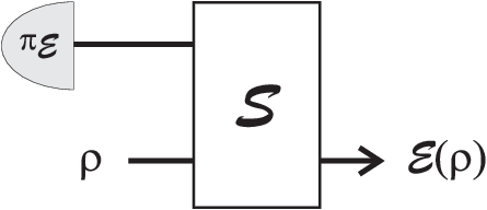
A quantum channel $\mathcal{E}$ is called programmable if there is a “simulator” $\mathcal{S}$ (another quantum channel) and a program state $\pi_{\mathcal{E}}$, such that

This is also shown in Fig. 3. Without loss of generality, the channel simulator can always be dilated into a unitary $U$ up to introducing extra degrees of freedom in the program state. Then we also say that an ensemble of channels $\Omega$ is “co-programmable” if the simulator $\mathcal{S}$ is universal over $\Omega$. In other words, for any $\mathcal{E}\in\Omega$, we may write Eq. (9) with exactly the same $\mathcal{S}$ but generally-different program states $\pi_{\mathcal{E}}$.

Let us now apply these notions to parameter estimation. Assume that the parametrised quantum channel $\mathcal{E}_{\theta}$ spans a family of co-programmable channels, so that we may write the simulation

We can then simplify any adaptive protocol over $n$ uses of this channel. In fact, we may replace each instance of the channel with its simulation of Fig. 3, so that the quantum comb in Fig. 2 can be re-organised in the form depicted in Fig. 4. The idea is to replace each use of the channel $\mathcal{E}_{\theta}$ with its program state $\pi_{\mathcal{E}_{\theta}}$, and then to “stretch” all the program states back in time, while collapsing the simulators $\mathcal{S}$ and the quantum comb (including its initial state $\sigma$) into a single quantum channel $\Lambda$. In this way, the output of the comb can be decomposed as

Note that the latter decomposition reduces the adaptive protocol into a block protocol up to an overall quantum channel $\Lambda$. Because of the properties of the QFI, we know that this is sufficient to restrict the performance of the protocol to the SQL. In fact, using monotonicity and additivity of the QFI, we may write

We have thus obtained that for the estimation of a parameter $\theta$ encoded in a programmable channel $\mathcal{E}_{\theta}$, the QCRB must satisfy the condition $\delta\theta^{2}\geq[n\mathrm{QFI}(\pi_{\mathcal{E}_{\theta}})]^{-1}$. Furthermore, note that this bound is not necessarily achievable. It would be achievable if the program state $\pi_{\mathcal{E}_{\theta}}$ could be generated by sending some input state through the channel. For instance, this would be the case if $\pi_{\mathcal{E}_{\theta}}$ were the Choi matrix of the channel, an extra property which is guaranteed if the channel is teleportation-covariant, as explained in the next section.

Before proceeding, we may ask how the channel simulation should be modified in order to cover channels that beat the SQL. One potential idea is to weaken the notion of co-programmability to involve multi-copy program states. For instance, suppose that a quantum channel $\mathcal{E}_{\theta}$ cannot be simulated as in Eq. (10) but as

This leads to the stretching $\rho_{\theta}^{n}=\Lambda(\pi_{\mathcal{E}_{\theta}}^{\otimes mn})$ and therefore to

We know that the HL $\delta\theta^{2}\gtrsim n^{-2}$ cannot be beaten so that we must have $m\leq n$. To get the HL it is sufficient that the condition in Eq. (13) holds asymptotically, i.e., in trace norm limit $\delta_{m}:=||\mathcal{E}_{\theta}(\rho)-\mathcal{S}(\rho\otimes\pi_{\mathcal{E}_{\theta}}^{\otimes m})||\overset{m}{\rightarrow}0$. Then we may take this limit jointly with the limit in $n$ for the scaling.

Teleportation simulation has been used in the past to reduce protocols of quantum communication into entanglement distillation [55, 56, 57, 58] and, more recently, to completely simplify protocols of private communication from adaptive to block forms [45], establishing the ultimate limits of QKD in point-to-point lossy communications [45] and also multi-point [59] and repeater-assisted scenarios [60]. More recently, Ref. [42] extended the technique to quantum metrology and quantum channel discrimination.

Let us start with discrete-variable systems and, in particular, qubits (arguments can be easily generalised to any finite dimension). We first recall the basic ingredients of teleportation and then we discuss how these can be modified to implement a tool of channel simulation. The standard qubit teleportation protocol [5, 61] can be broken down in three steps:

(1) Resource.

A maximally-entangled state $|\Phi_{+}\rangle=(|00\rangle+|11\rangle)/\sqrt{2}$ is prepared for qubits $A$ (Alice) and $B$ (Bob).

(2) Bell detection.

Alice performs a Bell detection on qubit $A$ and an input qubit $a$ (in an arbitrary state $\rho$). Recall that the Bell detection has four outcomes $\alpha\in\{0,1,2,3\}$ with POVM elements $|\Phi_{\alpha}\rangle\langle\Phi_{\alpha}|$ where $|\Phi_{\alpha}\rangle=(I\otimes\sigma_{\alpha})|\Phi_{+}\rangle$ and $\sigma_{\alpha}$ are the four Pauli unitaries [1]

		$\displaystyle\sigma_{0}=I:=\left(\begin{array}[c]{cc}1&0\\ 0&1\end{array}\right),\,\,\sigma_{1}=X:=\left(\begin{array}[c]{cc}0&1\\ 1&0\end{array}\right),$
		$\displaystyle\sigma_{2}=Y:=\left(\begin{array}[c]{cc}0&i\\ -i&0\end{array}\right),\,\,\sigma_{3}=Z:=\left(\begin{array}[c]{cc}1&0\\ 0&-1\end{array}\right).$

(3) Pauli corrections.

Finally, depending on the output of the Bell measurement $\alpha$, the conditional Pauli unitary $\sigma_{\alpha}^{-1}$ is applied on the qubit $B$, retrieving the input state $\rho$.

The standard teleportation protocol simulates the identity channel. A modification of the protocol is to employ a resource state which is not maximally-entangled but an arbitrary bipartite state. In this way teleportation implements not the identity but simulates a noisy channel from the input qubit $a$ to the output qubit $B$. Suppose that we choose the resource state to be the Choi matrix of a quantum channel $\mathcal{E}$, i.e.,

By teleporting over this state can we simulate channel $\mathcal{E}$?

The answer is yes for so-called teleportation-covariant channels [57, 58, 45]. By definition a quantum channel $\mathcal{E}$ is teleportation-covariant if, for any random teleportation unitary $U$ (corresponding to a Pauli operator in the qubit case), we may write

for some other unitary $V$ [45]. This property is a sufficient condition to ensure that the channel $\mathcal{E}$ can be simulated by teleporting over its Choi matrix or Choi-Jamiolkowski (CJ) state $\xi_{\mathcal{E}}^{\text{CJ}}$ (this is also known as teleportation-simulable or Choi-stretchable channel [45]). In other words, we may write the simulation [45, 42]

where $\mathcal{T}$ is teleportation. See Fig. 5 for a visual proof of Eq. (25). This is clearly a powerful design but only holds for the teleportation-covariant subset of programmable channels.

In the setting of quantum parameter estimation, we are interested in joint teleportation-covariance, where a parametrised quantum channel $\mathcal{E}_{\theta}$ satisfies Eq. (24) with a $\theta$-independent set of output unitaries, i.e., [42]

This is exactly the situation when $\theta$ is a noise parameter, i.e., a parameter that can be uniquely associated to an environment dilating the quantum channel.

If Eq. (26) holds, then we can write $\mathcal{E}_{\theta}(\rho)=\mathcal{T}(\rho\otimes\xi_{\mathcal{E}_{\theta}}^{\text{CJ}})$ and repeat the stretching of a quantum comb as before. In this way, we may decompose the output state of an adaptive parameter estimation protocol as [42]

for some quantum channel $\Lambda$. As a result, we get

This means that the estimation of a noise parameter of a teleportation-covariant channel is limited to the SQL with a pre-factor given by its Choi matrix, i.e., the QCRB reads [42]

The teleportation simulation not only allows us to compute explicitly the upper bound, but also yields a matching lower bound. As a matter of fact, an optimal strategy that saturates the bound employs a block (assisted) estimation protocol where the maximally-entangled state $\Phi_{+}$ is used at the input of the channel in an identical and independent way. This strategy provides a QFI exactly equal to $n\mathrm{QFI}(\xi_{\mathcal{E}_{\theta}}^{\text{CJ}})$. As a result, the QCRB in Eq. (29) is asymptotically achievable for large $n$.

Let us compute the QCRB for specific examples. It is known that erasure, dephasing and depolarizing channels are teleportation-covariant [45]. More precisely, these channels satisfy the condition of joint teleportation covariance of Eq. (26) with $\theta$ being their channel-defining probability parameter $p$. Recall that an erasure channel is represented by [1]

where $\left|e\right\rangle$ is an orthogonal erasure state and $p$ is the erasure probability. A dephasing channel is defined as [1]

where $p$ is the probability of phase flip. Finally, a depolarizing channel with probability $p$ is defined as [1]

where $\pi$ is the maximally-mixed state.

For each family of these channels $\mathcal{E}_{p}$ (i.e., erasure, dephasing or depolarizing), we compute the Choi matrix $\xi_{\mathcal{E}_{p}}^{\text{CJ}}$ and the associated QFI, finding $\mathrm{QFI}(\xi_{\mathcal{E}_{p}}^{\text{CJ}})=[p(1-p)]^{-1}$ for each of the families. Then, using Eq. (29), we find that the adaptive estimation of $p$ is bounded by the following asymptotically-achievable QCRB [42]

Here we present an alternative simulation for single-mode bosonic Gaussian channels which does not need to consider the limit of an asymptotic Choi matrix (but still requires the limit of an ideal Bell detection). Consider a two-mode Gaussian state with zero mean and generic CM

By teleporting over this Gaussian resource using a Braunstein-Kimble protocol with gain $g$ we obtain a Gaussian teleportation channel such that [46] $\mathbf{\bar{x}}\rightarrow g\mathbf{\bar{x}}$ and

where $\mathbf{Z}=\mathrm{diag}(1,-1)$. Therefore, a phase-insensitive Gaussian channel $\mathcal{E}_{\eta,\nu}$ with parameters $\eta$ and $\nu$ [see Eqs. (54) and (55) with $\mathbf{d}=\mathbf{0}$] can be simulated by using the gain $g=\sqrt{\eta}$ and using a CM $\mathbf{V}_{AB}$ with the choice

so that $\nu=ag^{2}-2cg+b$ [46].

We are interested in finding a finite-energy resource state $\sigma_{\nu}$ that can simulate a phase-insensitive Gaussian channel $\mathcal{E}_{\eta,\nu}$ according to

where $\mathcal{T}_{\eta}$ is the Braunstein-Kimble protocol with ideal Bell detection and gain $g=\sqrt{\eta}$. More precisely, we may write $\mathcal{T}_{\eta}=\lim_{\mu}\mathcal{T}_{\mu}^{\eta}$, where $\mathcal{T}_{\mu}^{\eta}$ is the Braunstein-Kimble $\mu$-protocol with gain $g=\sqrt{\eta}$. A possible choice for $\sigma_{\nu}$ is a Gaussian state with zero mean and CM

with the following elements

where

It is worth remarking that there exist many finite-energy resource states that can simulate a given channel. A different family of resource states has been obtained in Ref. [46] to characterise the teleportation fidelity. This family of resource states has also been exploited in quantum communication [70] to derive weak converse upper bounds for the secret key capacity of phase-insensitive Gaussian channels. These bounds closely approximate the ideal and tightest bounds obtained for infinite energy [45]. In what follows we use the sub-optimal simulation of Eq. (61) with the finite-energy resource state specified by Eqs. (62)-(64). It is the first time that this finite-resource approach is used in quantum metrology.

Note that the form of the simulation in Eq. (61) is such that the noise parameter $\nu$ only appears in the resource state $\sigma_{\nu}$ or, in other words, the teleportation LOCC $\mathcal{T}_{\eta}$ does not depend on $\nu$. For this reason, the family of channels $\mathcal{E}_{\eta,\nu}$ with fixed $\eta$ but varying $\nu$ is a family of jointly teleportation-simulable channels (which is a condition implied by the joint teleportation covariance). As a result, the adaptive estimation of the parameter $\nu$ can be completely simplified, so that the $n$-use output state of a comb reads $\rho_{\nu}^{n}=\Lambda_{\eta}(\sigma_{\nu}^{\otimes n})$ for some global quantum channel $\Lambda_{\eta}$ which is independent from the unknown parameter $\nu$. As a consequence, we may simplify the QFI of the output state $\rho_{\nu}^{n}$ and write the following QCRB for the adaptive estimation of $\nu$

As an example consider the additive-noise Gaussian channel $\mathcal{E}_{\nu}^{\text{add}}$. This channel can be simulated by exploiting a resource state $\sigma_{\nu}$ whose CM is given by Eq. (62)-(64) with $\eta=1$ (see also Refs. [71, 72]). We may then compute the QFI from the quantum fidelity [50], and find the QCRB $\delta v^{2}\geq v^{2}/n$. Note that this exactly coincides with the tight achievable bound of Eq. (57) which is obtained by simulating the channel via its asymptotic Choi matrix.

Consider now the adaptive estimation of the thermal number $\bar{n}$ of a thermal-loss channel $\mathcal{E}_{\eta,\bar{n}}^{\text{loss}}$ assuming the sub-optimal simulation. Putting $\nu=(1-\eta)(\bar{n}+1/2)$ in Eq. (65) we compute the QCRB for $\delta\bar{n}^{2}$. We do not find the tight achievable bound of Eq. (56) but a larger bound given by

For comparison, in Fig. 6 we plot the QFI for the asymptotic and finite-energy resource state. It is a open problem to find a finite-energy resource that can match the asymptotic bound. Finally, one may easily check that Eq. (66) also holds for a noisy amplifier $\mathcal{E}_{\eta,\bar{n}}^{\text{amp}}$ assuming its sub-optimal simulation.

Channel simulation is a powerful tool for completely simplifying protocols of adaptive parameter estimation, for instance represented as a quantum comb. This technique allows one to compute the ultimate precision in estimating noise parameters that are encoded in discrete- or continuous-variable channels. The tool easily applies to any programmable channel whose unknown parameter is encoded in its program (environmental) state. One can then reduce an adaptive protocol and show that the QCRB is limited to the SQL.

When a programmable channel is teleportation-covariant (such as an erasure, a Pauli or a Gaussian channel), we can exploit a precise design for its simulation which is based on a simple modification of the teleportation protocol. In this way, we may show that the QCRB is limited to the SQL with the QFI being computed on the Choi matrix of the channel (in an asymptotic fashion for bosonic Gaussian channels). Furthermore, the QCRB is shown to be achievable by a block (i.e., non-adaptive) protocol based on entanglement-assistance.

As a consequence of the previous results, a quantum channel able to beat the SQL and potentially reach the Heisenberg scaling must be necessarily non-programmable in the sense discussed in this review, i.e., it cannot be perfectly simulated by means of a single-copy program state. A potential approach to cover this type of channel is therefore considering an extended definition of multi-programmability where the simulation is achieved by using a multi-copy resource state.

In conclusion, we have reviewed the state-of-the-art in the theory of channel simulation within the context of quantum parameter estimation. The reader interested in similar applications in quantum channel discrimination may consult Ref. [42] and a forthcoming review paper [73]. The reader interested in applications to quantum and private communications (e.g., for establishing two-way capacities) may consult Ref. [64] and also one of the founding papers [45].

Acknowledgments. This work has been supported by the Innovation Fund Denmark (Qubiz project), the European Union (MSCA-IF-2016), and the EPSRC via the ‘UK Quantum Communications Hub’ (EP/M013472/1). S. P. thanks R. Demkowicz-Dobrzański, S. Lloyd, L. Maccone, J. Kolodynski, D. Braun, and G. Adesso for feedback on these topics.

References

- [1] M. A. Nielsen and I. L. Chuang, Quantum Computation and Quantum Information (Cambridge University Press, Cambridge, 2000).
- [2] C. Weedbrook, S. Pirandola, R. García-Patrón, N. J. Cerf, T. C. Ralph, J. H. Shapiro, and S. Lloyd, Rev. Mod. Phys. 84, 621 (2012).
- [3] F. Caruso, V. Giovannetti, C. Lupo, and S. Mancini, Rev. Mod. Phys. 86, 1203 (2014).
- [4] U. L. Andersen, J. S. Neergaard-Nielsen, P. van Loock, and A. Furusawa, Nature Phys. 11, 713 (2015).
- [5] C. H. Bennett, G. Brassard, C. Crépeau, R. Jozsa, A. Peres, and W. K. Wootters, Phys. Rev. Lett. 70, 1895 (1993).
- [6] L. Vaidman, Phys. Rev. A 49, 1473 (1994).
- [7] S. L. Braunstein and H. J. Kimble, Phys. Rev. Lett. 80, 869 (1998).
- [8] S. Pirandola, J. Eisert, C. Weedbrook, A. Furusawa, and S. L. Braunstein, Nat. Photon. 9, 641 (2015).
- [9] H. J. Kimble, Nature 453, 1023 (2008).
- [10] S. Pirandola and S. L. Braunstein, Nature 532, 169 (2016).
- [11] N. Gisin, G. Ribordy, W. Tittel, and H. Zbinden, Rev. Mod. Phys. 74, 145 (2002).
- [12] E. Diamanti and A. Leverrier, Entropy 17, 6072 (2015).
- [13] V. C. Usenko and R. Filip, Entropy 18, 20 (2016).
- [14] C. H. Bennett and G. Brassard. Quantum Cryptography: Public Key Distribution and Coin Tossing, Proceedings of IEEE International Conference on Computers, Systems and Signal Processing, pp. 175-179 (1984).
- [15] A.K. Ekert, Phys. Rev. Lett. 67, 661 (1991).
- [16] M. Lucamarini and S. Mancini, Phys. Rev. Lett. 94, 140501 (2005).
- [17] S. L. Braunstein, and S. Pirandola, Phys. Rev. Lett. 108, 130502 (2012).
- [18] F. Grosshans, G. Van Ache, J. Wenger, R. Brouri, N. J. Cerf, and P. Grangier, Nature 421, 238 (2003).
- [19] C. Weedbrook, A. M. Lance, W. P. Bowen, T. Symul, T. C. Ralph, and P. K. Lam, Phys. Rev. Lett. 93, 170504 (2004).
- [20] S. Pirandola, S. Mancini, S. Lloyd, and S. L. Braunstein, Nat. Phys. 4, 726 (2008).
- [21] S. Pirandola, C. Ottaviani, G. Spedalieri, C. Weedbrook, S. L. Braunstein, S. Lloyd, T. Ghering, C.S. Jacobsen, and U. L. Andersen, Nat. Photon. 9, 397 (2015).
- [22] S. Lloyd, Science 321, 1463 (2008).
- [23] S.-H. Tan, B. I. Erkmen, V. Giovannetti, S. Guha, S. Lloyd, L. Maccone, S. Pirandola, and J. H. Shapiro, Phys. Rev. Lett. 101, 253601 (2008).
- [24] S. Barzanjeh, S. Guha, C. Weedbrook, D. Vitali, J. H. Shapiro, and S. Pirandola, Phys. Rev. Lett. 114, 080503 (2015).
- [25] C. Weedbrook, S. Pirandola, J. Thompson, V. Vedral, and M. Gu, New J. Phys. 18, 043027 (2016).
- [26] M. Tsang, R. Nair, and X. Lu, Phys. Rev. X 6, 031033 (2016).
- [27] C. Lupo and S. Pirandola, Phys. Rev. Lett. 117, 190802 (2016).
- [28] R. Nair, and M. Tsang, Phys. Rev. Lett. 117, 190801 (2016).
- [29] S. L. Braunstein and C. M. Caves, Phys. Rev. Lett. 72, 3439 (1994).
- [30] P. Kok, S. L. Braunstein, and J. P. Dowling, J. Op. B 6, 8 (2004).
- [31] V. Giovannetti, S. Lloyd, and L. Maccone, Science 306, 1330 (2004).
- [32] H. M. Wiseman and G. J. Milburn, Quantum Measurement and Control (Cambridge University Press, 2010).
- [33] M. G. A. Paris, Int. J. Quant. Inf. 7, 125 (2009).
- [34] V. Giovannetti, S. Lloyd, and L. Maccone, Nature Photon. 5, 222 (2011).
- [35] G. Toth and I. Apellaniz, J. Phys. A: Math. Theor. 47, 424006 (2014).
- [36] D. Braun, G. Adesso, F. Benatti, R. Floreanini, U. Marzolino, M. W. Mitchell, and S. Pirandola, Quantum enhanced measurements without entanglement, arXiv:1701.05152 (2017).
- [37] M. A. Nielsen and Isaac L. Chuang, Phys. Rev. Lett. 79, 321 (1997).
- [38] Z. Ji, G. Wang, R. Duan, Y. Feng, and M. Ying, IEEE Trans. Info. Theory 54, 5172 (2008).
- [39] K. Matsumoto, On metric of quantum channel spaces, arXiv:1006.0300v1 (2010).
- [40] J. Kolodyński and R. Demkowicz-Dobrzański, New J. Phys. 15 073043 (2013).
- [41] R. Demkowicz-Dobrzański and L. Maccone, Phys. Rev. Lett. 113, 250801 (2014).
- [42] S. Pirandola, and C. Lupo, Phys. Rev. Lett. 118, 100502 (2017); ibidem 119, 129901 (2017).
- [43] R. Demkowicz-Dobrzański, J. Czajkowski, and P. Sekatski, Phys. Rev. X 7, 041009 (2017).
- [44] S. Zhou, M. Zhang, J. Preskill, and L. Jiang, Achieving the Heisenberg limit in quantum metrology using quantum error correction, arXiv:1706.02445 (2017).
- [45] S. Pirandola, R. Laurenza, C. Ottaviani, and L. Banchi, Nat. Commun. 8, 15043 (2017).
- [46] P. Liuzzo-Scorpo, A. Mari, V. Giovannetti, and G. Adesso, Phys. Rev. Lett. 119, 120503 (2017).
- [47] G. Chiribella, G. M. D’Ariano, and P. Perinotti, Phys. Rev. Lett. 101, 060401 (2008).
- [48] A. Uhlmann, Rep. Math. Phys. 9, 273 (1976).
- [49] R. Jozsa, Journal of Modern Optics 41, 2315 (1994).
- [50] L. Banchi, S. L. Braunstein, and S. Pirandola, Phys. Rev. Lett. 115, 260501 (2015).
- [51] S. Ishizaka and T. Hiroshima, Phys. Rev. Lett. 101, 240501 (2008).
- [52] S. Ishizaka and T. Hiroshima, Phys. Rev. A 79, 042306 (2009).
- [53] S. Ishizaka, Some remarks on port-based teleportation, arXiv:1506.01555 (2015).
- [54] W. Zhi-Wei and S. L. Braunstein, Sci. Rep. 6, 33004 (2016).
- [55] C. H. Bennett, D. P. DiVincenzo, J. A. Smolin, W. K. Wootters, Phys. Rev. A 54, 3824 (1996).
- [56] M. M. Wolf, Notes on Quantum Channels and Operations (2012).
- [57] A. Muller-Hermes, Transposition in quantum information theory (Master’s thesis, Technical University of Munich, 2012).
- [58] D. Leung and W. Matthews, IEEE Trans. Info. Theory 61, 4486 (2015).
- [59] R. Laurenza and S. Pirandola, Phys. Rev. A 96, 032318 (2017).
- [60] S. Pirandola, Capacities of repeater-assisted quantum communications, arXiv:1601.00966 (2016).
- [61] S. Pirandola and S. Mancini, Laser Physics 16, 1418 (2006).
- [62] G. Giedke and J. I. Cirac, Phys. Rev. A 66, 032316 (2002).
- [63] J. Niset, J. Fiurasek, and N. J. Cerf, Phys. Rev. Lett. 102, 120501 (2009).
- [64] S. Pirandola, S. L. Braunstein, R. Laurenza, C. Ottaviani, T. P. W. Cope, G. Spedalieri, and L. Banchi, Theory of channel simulation and bounds for private communication, arXiv:1711.09909 (2017).
- [65] A. Furusawa, J. L. Sørensen, S. L. Braunstein, C. A. Fuchs, H. J. Kimble, and E. S. Polzik, Science 282, 706 (1998).
- [66] S. L. Braunstein, G. M. D’Ariano, G. J. Milburn, and M. F. Sacchi, Phys. Rev. Lett. 84, 3486 (2000).
- [67] A. S. Holevo, Probab. Theory Appli. 48, 243 (2004).
- [68] M. E. Shirokov, Energy-constrained diamond norms and their use in quantum information theory, arXiv:1706.00361 (2017).
- [69] F. Caruso, V. Giovannetti, A. S. Holevo, New J. Phys. 8, 310 (2006).
- [70] R. Laurenza, S. L. Braunstein, and S. Pirandola, arXiv: 1706.06065 (2017).
- [71] M. Ban, M. Sasaki, and M. Takeoka, J. Phys. A 35, L401 (2002).
- [72] A. Christ, C. Lupo, and C. Silberhorn, New J. Phys. 14, 083007 (2012).
- [73] S. Pirandola, B. R. Bardhan, T. Gehring, C. Weedbrook, and S. Lloyd, Advances in quantum sensing, in preparation (2017).