Driving Spin-Boson Models From Equilibrium Using Exact Quantum Dynamics
Abstract
We present an application of the Extended Stochastic Liouville Equation (ESLE) [Phys. Rev. B 95, 125124], which gives an exact solution for the reduced density matrix of an open system surrounded by a harmonic heat bath. This method considers the extended system (the open system and the bath) being thermally equilibrated prior to the action of a time dependent perturbation, as opposed to the usual assumption that system and bath are initially partitioned. This is an exact technique capable of accounting for arbitrary parameter regimes of the model. Here we present our first numerical implementation of the method in the simplest case of a Caldeira-Leggett representation of the bath Hamiltonian, and apply it to a spin-boson system driven from coupled equilibrium. We observe significant behaviours in both the transient dynamics and asymptotic states of the reduced density matrix not present in the usual approximation.
I Introduction
The coupling of an environment to a system introduces phenomena not found in isolation. In particular, dissipation, Brownian fluctuations and (in the quantum case) decoherence cannot be observed or explicated without recourse to environments [1]. It is an essential component of quantum thermodynamics [2, 3], and vital to the field of quantum computing, where coherence is a resource which the environment can dissipate [4, 5, 6] or enhance (with suitable environmental engineering) [7].
Historically, methods based on the Feynman-Vernon influence functional [8] have had great success in the treatment of environmental effects [9, 10, 11, 12, 13, 14, 15, 16]. In this formalism, the extended system-environment Hamiltonian (consisting of the contributions due to the open system, the environment and their coupling) is cast as a path integral, where the environment can be analytically integrated over to give an expression for the reduced density matrix, representing the open system purely in terms of the open system operators. This results in a modified propagator for the open system, where the effect of the environment and its interaction with the open system is captured by additional terms in the path integral exponent known as the influence functional. In this approach the inital density matrix is factorised, i.e. it is assumed that the open system and its environment are initially partitioned and hence there is no interaction between them at the initial time [17].
From this representation, a number of techniques have been developed. A few examples are the Stochastic Schrodinger Equation [18, 19], Stochastic Liouville-von Neumann Equation [20] and the quasiadiabatic path integral [21]. While these techniques have been applied to a broad range of problems, the spin-Boson model has proved a particularly popular test-bed [22, 23, 2, 18, 19, 24]. This model has also been interrogated by other methods, including cumulant expansions [25], matrix products [26] and reaction-coordinate [27] approaches. It is also amenable to analytic derivations, both perturbatively [28] and nonpertubatively [29], as well as to an application of the Born approximation [30]. The model may also draw on the extensive work done on driven two-state models, most famously the Landau-Zener sweep [31, 32, 33] and its generalisations [34, 35, 36].
In addition, the spin-Boson model displays rich, non-trivial behaviour, with integrable and non-integrable regimes [37], diffusive and localised phases [38], as well as coherent to incoherent crossovers [39, 40]. Besides the model’s obvious application to qubit behaviour, it has been mapped to impurities in an electronic bath (i.e. Kondo model) [41, 42], Josephson junctions [43, 44], cold atoms [45, 23], and even biological systems [46]. The spin-Boson model therefore serves as an excellent toy model, with application to real experimental systems.
The main assumption made in the work mentioned above is that initially the extended system is partitioned, i.e. the open system and bath are initially non-interacting. The interaction betwen the open system and bath is then turned on for the dynamical evolution. This, so-called partitioned approach, strictly speaking, is only applicable for weak system-bath coupling, as well as when studying the long-time behaviour when transient effects due to the unphysical initial preparation of the system die away. Our recent work introduced the Extended Stochastic Liouville Equation (ESLE) method [47], which enables one to project out the environment exactly, without assuming that it is decoupled from the open system at the initial time. The ESLE is a non-perturbative, exact set of stochastic differential equations for the reduced density matrix of the open system, in which the role of the environment is played by Gaussian stochastic processes in real and imaginary time which “replace” its harmonic oscillators. It also includes an imaginary time evolution to exactly account for the chosen thermal equilibrium initial condition (although a broader class of initial conditions can also be introduced [10]), and allows for a simple and general closed form description of the evolution of the reduced density matrix. In particular, it is able to faithfully capture the transient dynamics of driving the system away from the full system-environment equilibrium caused by any local (acting only on the open system), and possibly time-dependent, perturbation. Hence, in this method one starts from the equilibrium density matrtix of the entire system at a certain temperature , and then considers exact time evolution of the open system reduced density matrix under the influence of an arbitrary system-local perturbation switched on at a particular time.
While the general proof in Ref. [47] showed that a reduced description of the open system is possible, the feasibility of numerical implementation nor resulting simulations were presented. This paper represents the first application of the ESLE method to a calculation in silico. Our aim here is (i) to introduce a numerical implementation of the ESLE; more specifically, we explain how the noises, cross-correlated with each other, can be generated on a computer, and (ii) apply this formalism to a spin-boson system driven from equilibrium, with particular attention paid to how the ESLE modifies the predicted short-time evolution and how its solution at long times depends on the initial preparation of the system.
The rest of this paper will be structured as follows: Sec. II briefly introduces the ESLC method to provide the essential theoretical basis needed, which is then applied to a simplified Hamiltonian that enables us to reduce the ESLE description to only three Gaussian noises. In Sec. III methods used to generate the noise terms in the ESLE are discussed. Sec. IV presents the spin-Boson Hamiltonian and results of the simulations using the ESLE, and we close with a discussion in Sec. V on the scope of the applications and current limitations of the ELSE.
II Extended Stochastic Liouville Equation
General theory
In our model the open system (denoted by a general argument ) is described by an arbitrary Hamiltonian (which could be time-dependent), while the environment is described by a set of harmonic oscillators (with masses ), with a potential which is quadratic in their displacement coordinates . The interaction between the two subsystems is linear in environment coordinates , but may involve an arbitrary function of the open system coordinates, . Explicitly, the total quantum Hamiltonian is given by:
| (1) |
Here is the momentum operator conjugate to the displacement , and is the environment force-constant matrix. This Hamiltonian generalises the CL model in two ways: firstly, the coupling term is generalised from a bilinear in CL to a more general one (although still linear in the bath coordinates11 1 Note that a generalisation to a quadratic coupling (with respect to the atomic displacements ) is also possible, at least formally.); secondly, the environment model is written via the site representation, rather than via normal modes, which allows for a more natural extraction of the parameters of the bath Hamiltonian from the whole system Hamiltonian (see, e.g., [49]).
As mentioned in the Introduction, in most treatments considering dynamics of an open system it is assumed that at initial time the system and environment are partitioned, i.e. the full system-environment density matrix is the tensor product of the open system density matrix and the environment matrix :
| (2) |
As was demonstrated in our previous work [47], instead of the aforementioned partitioned approximation, the initial state of the system may be described by a preparation of the canonical density matrix for the extended system [10]:
| (3) |
where
| (4) |
is the initial canonical density matrix, is the initial Hamiltonian, is the inverse temperature and is the corresponding partition function of the entire system. Here is an operator acting only on the open system. Although this operator may be chosen in various ways to reflect specific initial conditions, in the present work we restrict ourselves to the system initially being in full thermal equilibrium, i.e. we choose .
With some elementary manipulations, it is possible to derive an exact evolution of the reduced density matrix describing the open system. The set of equations governing this evolution constitutes the ESLE (for full details see [47]). The ESLE consists of two stochastic operator evolutions, which, upon averaging over realisations of the Gaussian stochastic noises it contains (see below), give the exact open system (i.e. reduced) density matrix at any time . The first evolution is in imaginary time , evolving an initial density matrix from up to , via the following equation:
| (5) |
This is then followed by a real time evolution:
| (6) |
Here is the (anti-) commutator. The two equations are coupled via the condition that the end-point of the imaginary evolution is the initial condition for the real-time stochastic dynamics:
| (7) |
To initialise the evolution of , we start with , evolve it in time and then normalise to unity at the end of the evolution.
The functions and () are zero-mean, complex, Gaussian noises in real (imaginary) time, and the actual (physical) reduced density matrix of the open system is obtained by averaging over all realisations (indicated by ) of these noise processes:
| (8) |
The origin of the noise comes from the application of a two-time Hubbard-Stratonovich transformation [50] to the influence functional derived for the environment. This provides an exact mapping of deterministic, temporally non-local dynamics to a stochastic, local model, provided the noise correlation functions satisfy the following conditions:
| (9) |
| (10) |
| (11) |
| (12) |
| (13) |
where is the Heaviside function and the various kernels are given by:
| (14) |
| (15) |
| (16) |
| (17) |
| (18) |
Here are the eigenvectors of the dynamical matrix of the environemnt, where , with eigenvalues .
Note that for a partitioned initial condition, there is no coupling between the open system and environment at . This approach is formally equivalent to neglecting the imaginary time evolution (setting ) and removing cross-correlations between the real and imaginary time evolutions (i.e. setting to zero for all and ). The initial density matrix of the open system, , can then be chosen arbitrarily. This choice may be based on physical insight or alternately as a solution of the imaginary time evolution, Eq. (5). In the latter case it would correspond to the exact reduced density matrix for the thermalised extended system.
A simplified model
The prescription considered so far requires three noises ( and ) per bath lattice site . Alternatively, one can use the eigenstates of the dynamical matrix and normal modes instead of the site representation. Formally we replace , , , and , which reduces the description to the standard Caldeira-Leggett model [1] albeit with a slightly more general coupling term, . In this representation all the correlation function matrices become diagonal, e.g.
The main simplification then comes by assuming that, up to a scaling factor, the dependences in the coupling functions are identical, i.e. . In this prescription it is possible to collectively redefine the noise terms reducing them to just three distinct terms. Taking the noises in Eq. (6) as an example:
| (19) |
with . The correlation function of this combined noise will be given by:
| (20) |
In the continuum limit we can replace the sum over bath modes with an integration over frequency:
| (21) |
Here is the bath spectral density, which is formally chosen depending on the specific model which couples oscillators of the environment and the system. In this paper we shall use an Ohmic spectral density, given by:
| (22) |
where is some cut-off frequency. The parameter is proportional to squares of the coefficients and hence describes the effective bath coupling strength.
Similarly to the noise, two other collective noises, and , are introduced, giving three noises in total. In the reduced case, which we shall use in the rest of the paper, the ESLE can be completely described by two stochastic differential equations, one for the initialisation in the imaginary time,
| (23) |
and another for the propagation in real time:
| (24) |
where the corresponding correlation functions are given by the following equations:
| (25) |
| (26) |
| (27) |
| (28) |
| (29) |
While this set of equations represents an exact description, it requires the generation of noises in two different time dimensions, which obey the specific statistical relationships detailed above. The numerical implementation of these noises will now be discussed.
III Generating Noises
The numerical scheme for the ESLE is in principle rather simple, illustrated by Fig. 1. The proceduce is to generate a realisation of the noises satisfying Eqs. (25)-(29), evolve the density matrix according to Eqs. (23) and (24), and finally average over realisations, Eq. (7). In this section we shall discuss how the three noises are generated; the method used can easily be generalised to any number of noises.
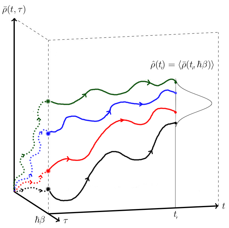
The general scheme to generate coloured Gaussian noises is well known [51], and the situation is only slightly complicated by the existence of ESLE’s non-stationary cross-time correlations. We begin by splitting each noise into sub-terms which are only correlated with one other term across the noises:
| (30) |
| (31) |
| (32) |
For instance, the noise is the auto-correlative part of the total noise, and has a non-zero correlation only with itself, while the noise only correlates with the term. To enforce this effective “noise-orthogonality”, we express each term as a convolution between a filtering kernel (which are denoted as , , etc.) and one of a number of real white noise processes , which have the property:
| (33) |
| (34) |
| (35) |
Given that the time (real or imaginary) is simply a parameter in the noise process, the distinction between and is one of notational convenience, rather than an expression of any fundamentally dissimilar statistics. The various components of the three complex noises we need are generated by the following convolutions of the filtering kernels with the white noises:
| (36) |
| (37) |
| (38) |
| (39) |
| (40) |
| (41) |
Here the limits on integrations over imaginary time reflect the fact that is constrained to lie within the interval . In this construction the various filtering kernels are yet to be determined. Importantly, as the only physically relevant constraints on the noises are the physical kernels, this linear filtering ansatz will be valid provided we can establish a consistent mapping between the physical (see Eqs. (25) - (29)) and filtering kernels. Note that in all cases we assume the filtering kernels have the same stationarity properties (i.e. they depend only on time differences) as the corresponding physical kernels . Hence the cross-time correlation filtering kernels and , that are responsible for the cross-time correlation between real and imaginary times noises (see Eq. ([eq:newcrosstimekernelident]) later on) involves both real and imaginary times, are not assumed to be stationary, unlike the other filtering kernels.
It can easily be seen that, with the above choice, , , , and ; all other correlation functions are identically equal to zero because of the design imposed “orthonormality” of the white noises, Eqs. (33)-(35). For instance,
| (42) |
as by Eq. (29).
To find the correspondence between the physical and filtering kernels, we substitute the assumed functional form of each noise given above into their relations (25) - (29) with the physical kernels. Explicit evaluation of this auto-correlative component yields:
| (43) |
leading to the first of the kernel mappings:
| (44) |
The physical kernel is therefore expressible as a self-convolution of the filtering kernel, and can be further simplified using its Fourier representation:
| (45) |
This equation is the only constraint on , and any solution to this equation yields a valid filtering kernel. In this particular case the solution is unique (up to a phase), but we shall see later that cross-correlative mappings do not uniquely define the relevant filtering kernels, and hence some choice exists which can be exploited. Given that the physical kernel here is both real and symmetric, we may constrain the filtering kernel to have the same properties and express it simply as:
| (46) |
The auto-correlative component of the noise has the same properties as above, provided we extend the integration domain of Eq. (39) and periodically extend across this domain. Then the filtering kernel has an identical mapping in Fourier space:
| (47) |
There are also two non-zero cross-correlative terms to consider: the real time correlation between the and noises, and the cross-time correlation between and . In the first case, we have:
| (48) |
or in Fourier space:
| (49) |
Unlike with the auto-correlative processes, we are left with a degree of choice in the form of the two filtering kernels. Here we take the simple expedient of choosing one of the kernels as a delta function, or . The second filtering kernel may therefore be straightforwardly identified as:
| (50) |
We now turn our attention to the final cross correlation, for which we obtain:
| (51) |
In this case we cannot use the Fourier transformation to simplify the expression of the filtering kernels, as the physical kernel is inherently non-stationary. Once again it is convenient to set one kernel as a delta function, , giving the form of the other kernel as:
| (52) |
which completes the mapping between the physical and filtering kernels. Note that setting either of the filtering kernels or to zero results in the loss of correlations between the imaginary and real time evolutions, which essentially corresponds to the reduced SLE method with the initial density matrix obtained independently from the imaginary time evolution.
Armed with this mapping, the noises are straightforwardly generated by the convolution of filtering kernels with vectors of white noise (with variances appropriate to the discretisation of the timestep). Further details on the generation of these noises, as well as the numerical solution for the ESLE may be found in the Appendix.
Typical results for noise generation are shown in Fig. 2, demonstrating that excellent convergence to the physical kernels can be achieved, provided that a sufficient sampling is taken. In particular, the apparently noisier behaviour of is due to its relatively small range of values, and the fact that its cross-time correlative part must be generated with the cruder direct summation (see Appendix). Panel (f) shows the RMS deviation for the non-zero correlations as functions of the number of runs used to generate them; one can see that the overall error is sharply decreased with the number of runs.


IV Application to a Driven Spin-Boson Model
Spin-Boson Models
Consider a two-state system described by the (matrix) Hamiltonian:
| (53) |
Here describes the bias between states, while controls tunnelling between them; and are the usual Pauli spin-matrices. While using our formalism it would be possible to consider any spin-boson model, we shall focus here on two seperate protocols: (i) an equilibrium real time evolution when the bias is kept constant at the value used to thermalise the whole system during imaginary time evolution, and (ii) a Landau-Zener type sweep, where the system has been thermalised at some time in the past, , and then evolved with . In both cases the tunneling is kept constant. Rather than using an analytic result in the second case (none exists), the asymptotic limit will be extrapolated numerically from the initial state calculated by the ESLE. Given that the ESLE evolves from an explicit thermal state at finite temperature and there is no analytic expression available, including the one to describe its asymptotic behaviour, the two-state solution provides a useful numerical benchmark to evaluate the impact of the environment.
Coupling this two-state system to an environment of the standard CL type and using , the total Hamiltonian reads as:
| (54) |
This is simply the matrix form of the total Hamiltonian given in Eq. (1), with the appropriate model-specific substitutions and the second quantisation for the environment oscillators, where () is the bosonic annhilation (creation) operator. The last term corresponds to the system-environment coupling which is proportional to the normal mode displacements of the environment. The only explicit dependence in the total Hamiltonian is contained in the (possible) bias field for the open system.
To apply the ESLE to this system, we assume that the total system-environment is allowed initially (at time ) to thermalise having the Hamiltonian corresponding to some initial value of the bias. Explicitly:
| (55) |
This initial condition implies the following ESLE equations in imaginary () and real () times:
| (56) |
| (57) |
In other words, we consider the initial condition to be parametrised by with real-time dynamics either keeping that value of the bias (the first protocol) or linearly driving the system away from its thermal state (the second).
Finally, we should be precise in our definition of strong-coupling. This is usually measured by the parameter in the spectral density, Eq. (22). It has been shown that for there is a coherent evolution, but crossing through the point causes a phase change to incoherent spin dynamics [1, 52]. Beyond this at the system enters a localised regime where tunnelling between the two states is completely suppressed (formally the bath coupling renormalises the tunelling element to ). These behaviours are peculiar to the spin-boson model, and not indicative of a general restriction of the parameter space the ESLE is capable of simulating exactly. Our results will focus on the regime , where we should expect coherent, damped oscillations in the spin expectations.
Equilibrium
As a sanity check, we first test the ESLE for a time-independent bias. Given the ESLE is thermalised in imaginary time exactly, we expect the real-time evolution to show no change in the density matrix.
Figure 3 shows the density matrix components of both the ESLE, and a comparative simulation running the real time part of the ESLE without the cross-time correlations. This reduced case corresponds to the Stochastic Liouville Equation (SLE) [20] based on the partitioned approach. In the SLE we initialise the density matrix from two initial conditions: (i) and (ii) the density matrix predicted by the ESLE imaginary time evolution, =.
For both the ESLE and the SLE simulation initialised from the imaginary-time evolution end-point, small oscillations in the components are observed, but they remain on average constant. This demonstrates that the cross-time correlations in the ESLE have little to no effect at equilibrium. This is as expected: any cross-time correlations in the noise rapidly die out as the system evolves in real time, and the noises evolving the SLE and ESLE become statistically identical. If the SLE simulation (started from the ESLE initial condition) evolved differently to the ESLE, then the ESLE would echo that behaviour later in time- a manifestly unphysical scenario at equilibrium.

The SLE simulation initialised at shows a relaxation of the spin. It is expected that this relaxation will converge to the same steady state as predicted by the other simulations, but it does so on a timescale not fully accessible by our numerical scheme. This is due to the fact that in equilibrium, the cut-off frequency of the bath spectrum must be sufficiently large that any energy the spin system dissipates to the bath is returned in a finite time. If this is not the case thermal equilibrium is not possible, as the bath acts as an energy sink (causing the spin to relax). At the same time, from a numerical perpective, higher cut-off frequencies require a smaller time-step to avoid non-physical resonances. This is doubly problematic, as the timescale for the SLE to relax increases with cut-off frequency [53], while the stochastic simulation itself is step-limited. That is, numerical instabilities at longer times require excessive averaging to eliminate, i.e. many more simulations are needed for sampling, which is extremely demanding computationally. At lower cut-off frequencies, all simulations are observed to converge to the same state, but the ESLE displays an unphysical spin-relaxation from the thermalised state due to the low cut-off.
Landau-Zener Protocol
Here we shall consider fully non-equilibrium simulations, in which the bias is linearly driven from the value used for the equilibration (imaginary time evolution). This spin-boson model is particularly useful in this case, as for specific initial conditions the asymptotic behaviour can be analytically derived. In the zero temperature case, when the system is started in the state
| (58) |
and is decoupled from the environment oscillators, the asymptotic survival probability of that state is given by:
| (59) |
This protocol is known as the Landau-Zener (LZ) sweep, with first derived by Zener by recasting the system as a Weber equation [31]. The result may also be found via contour integration [32] or direct evaluation of the time-ordered propagator [33]. This protocol has numerous experimental realisations, for example in Rydberg atoms [54] or Bose-Einstein condensates [55]. It has also been proven that the survival probability for the state is the same even with a coupling to a dissipative environment (of the Caldeira-Leggett type), with the caveat that the total system must be prepared in the ground state at zero temperature and evolved from [56, 57]. Furthermore, numerical evaluations using a Stochastic Schrödinger Equation (SSE) have shown that even in the case where the evolution is started from some finite time sufficiently far in the past (for a fixed initial spin), provided the bath coupling is sufficiently weak , is still recovered at zero temperature [18]. At stronger couplings however deviations from in the asymptotic state were observed, confirming that generally even at zero temperature the asymptotic spin state in a dissipative system depends on both the bath coupling strength and the initial preparation of the system.
As our theory enables to provide an exact dynamics of the spin-boson system density matrix, it is interesting to explore the validity of the LZ sweep limit (59) in detail, both at finite temperature and with the envoronment coupling.
General time behaviour
To model the LZ type sweep, we thermalise the system at some time in the past with the bias and then evolve it in real time for . For the purposes of achieving a quicker relaxation to the asymptotic state, the cut-off frequency was chosen for all simulations. Unlike in the equilibrium case, where a large cut-off frequency was used to ensure the energy scale of the bath was always much greater than that of the spin, in the driven case in our simulations the system starts and ends with considerably stronger bias. As all the dynamical changes occur in a window around , the effect of reducing the cut-off frequency is to narrow the region where the state transitions may happen. In addition, we set , which means that effectively all parameters of the system are scaled to units of .
Fig. 4 shows an ESLE evolution of at finite temperature, where parameters were chosen such that the initial density matrix approaches that of the LZ initial condition, , although the evolution still begins from a finite time in the past. We expect that from this initial condition the cross-time correlations (which rapidly attenuate with time) are suppressed when evolving from a regime where the bias field is initially much stronger than thermal effects. This limiting case therefore also serves as a check that the ESLE predicts evolutions consistent with partitioned methods.
One can see that at finite temperatures the asymptotic behaviour does not necessarily converge to the LZ result even at weak coupling. In addition, while the mean state of the system rapidly converges to its asymptotic limit, the amplitude of oscillations around this state, and their rate of decay appears dependent on temperature, with oscillation amplitude decaying slower at lower temperatures. We also observe that the mean value approaches the LZ value as the temperature is lowered. This can be explained by the final state (and its convergence to the LZ limit) being dependent on the size of the temporal region where the bias field is comparable to the strength of thermal fluctuations. This region, where is when thermal effects will have the greatest impact on the dynamics of the system, as elsewhere the bias field dominates the system evolution. Therefore, we should expect the asymptotic state at lower temperature to lie closer to the LZ limit. Unfortunately, the time required for oscillations to decay sufficiently to confirm this is much longer at lower temperature. Given the excessive computational cost of longer simulation times in the ESLE (see Section V), in Fig. 4 the asymptotic states for the two lowest temperatures are extrapolated from (oscillating) data. From this we conclude that high temperatures (or slow sweeps) allow thermal effects to increase the asymptotic value away from , consistent with earlier SSE results [19].

Coupling-Strength Dependence
Fig. 5 (a) shows the real time dynamics of for the LZ sweep at different coupling strengths. Here simulations are started from a sufficiently small such that the calculated initial density matrices are distinguishable from . Comparing results in Fig. 5, we find that the bath coupling has two principal effects. First, oscillatory behaviour in the spin expectations is suppressed by increasing bath coupling, as expected. The asymptotic survival probability also increases, for the same reason as when increasing temperature. Indeed, stronger coupling allows thermal effects to have a stronger influence on the evolution lifting the asymptote. This phenomenon can also be understood as the system-bath coupling renormalising the characteristic frequency scale of oscillations, resulting in a quicker thermalisation. This scaling can be expressed in terms of the renormalised tunelling element [1, 58]:
| (60) |
Given this scaling is an argument based purely on renormalising the system Hamiltonian, we should expect it to hold regardless of the initial condition chosen. It should be noted here that the ESLE is at root a faithful representation for a particular kind of initial condition, and should not affect the dynamical properties of a system. Fig. 5 (b) shows the dynamics when time is scaled via this renormalised tunnelling element, demonstrating that the curves of varying scale on top of each other, hence serving as another consistency check that the ESLE produces physically reasonable results.


Comparison to Partitioned Evolution
We now compare the full ESLE to an SLE evolution purely in real time. Using the SLE, we may consider three different initial conditions:
- •
“SLE LZ”, where the system is evolved from the Landau-Zener initial condition: ;
- •
“SLE matched”, where the initial condition is that calculated from the averaged ESLE imaginary time evolution, i.e. from the exact reduced density matrix, , obtained by solving Eq. (56); this evolution differs from the exact ESLE only in that the cross-time correlation is set to zero;
- •
“SLE partitioned”, where the partitioned approximation is made to the initial state: .
Fig. 6 shows the ESLE solution compared to these three cases of the SLE at both (a,b) weak and (c,d) strong coupling. There are several points to note here. The first is that there is a small (but visible) difference between the initial condition calculated by the ESLE and the naive initial condition used by the“SLE partitoned” approach, particularly at strong coupling. All partitioned evolutions exhibit initial oscillations (which are damped by stronger coupling), particularly in the coherence . Its asymptotic state is also different to the ESLE at both coupling strengths. The partitioned simulation also displays greater numerical instability, particularly at strong coupling.
The SLE LZ partitioned simulation differs most from the ESLE in its transient dynamics. This is consistent with the ESLE’s cross-time correlations, which are expected to have the largest effect at the start of the real-time dynamics due to the decay of the corresponding correlation kernels (27) at longer times. To test whether the oscillations observed in this simulation are simply due to initial conditions, or if the cross-time correlations in the ESLE actually suppress these oscillations, we compare to the “SLE matched” initial preparation, which starts from the calculated ESLE initial density matirx but then neglects the cross-time correlations in its real time evolution.. Comparing this simulation to the ESLE we find cross-time correlations are responsible for damping small transient oscillations in the coherence (see 6(b)). From this we conclude that the main contributary factor in the observed difference between the ESLE and “SLE partitioned” is due the choice of initial condition.
Examining the long-time behaviour reveals a small gap between the asymptotic states of the ESLE and “SLE matched” that can only be due to the cross-time correlations missing in the SLE simulation. This indicates that the cross-time correlations have an observable effect not only on the transient dynamics, but on the asymptotic state as well. This is not surprising, given that the Landau-Zener steady state is known to depend on initial conditions as representing a continuing non-equilibrium evolution with time-dependent Hamiltonian.
Finally we note that the “SLE LZ” simulation gives an asymptotic value for significantly higher than the LZ limit. This is to be expected, given the high temperature simulated, and the relatively short time in the past the evolution is begun from.


V discussion
In this paper we have presented a numerical application of the exact ESLE to a driven spin-boson model.
While there are no analytic predictions for evolutions from the exact initial density matrix presented, the numerical solution for the spin-boson system dynamics considered here using our exact partitionless method have been found to be extremely important as it can serve as a reference when comparing with previous approximate calculations based on the partitioned approach. In the latter method, cross-correlations between system preparation (imaginary time evolution or thermalisation) and real time evolution are artificially missing. In this proof of concept for the method we have restricted ourselves to relatively short evolutions at high sweep speeds, to achieve quicker convergence of the results.
We have shown that for a simple system-bath coupling considered here only three Gaussian noises need to be generated: one for the imaginary time evolution that brings the entire system (the open system and the bath) to thermal equilibrium (initial preparation), and two functions for the real time evolution. The method presented here enabled us to generate these noises in such a way that all correlation functions are reproduced. We find, however, that small errors require very large sampling set, i.e. up to and over simulation runs are required to produce physically reasonable results.
As a sanity check of the method and its implementation, we first considered a real time evolution with a cons4tant system Hamiltonian. One would expect that the real time evolution with the exact density matrix obtained after thermalisation in imaginary time should remain unchanged, and this was indeed found to be the case: we have seen that the ESLE predicts no change from initial conditions in its real time evolution (as expected). SLE simulations from various initial conditions show relaxation, but on a timescale where we cannot reliably ascertain their steady state. Nevertheless, in the long time limit cross-time correlations die away, and both the ESLE and SLE will be evolved using noises with identical statistical properties, therefore we should expect the SLE simulation to converge to the ESLE result. At the same time, we find that great care is needed in achieving numerically acceptable results. This stems from the fact that the ESLE is a stochastic differential equation with multiplicative noise, as well as a first order finite difference approximation?. This inevitably leads to a limit on the number of steps it may efficiently simulate before numerical instabilities dominate. In the future a more sophisticated numerical implementation [59, 60] will help results to converge with a larger timestep and hence allow access to longer timescales.
In addition to the equilibrium simulation, the non-equilibrium problem of a Landau-Zener sweep (in which the bias in the open system Hamiltonian is linearly driven) was also simulated. The exact ESLE simulation is compared specifically with the approximate (partitioned) SLE approach in which only real time evolution is considered from a chosen initial density matrix. We observe significant differences between partitioned evolutions and the ESLE, particularly at stronger coupling. We have found that the asymptotic behaviour of the ESLE in a Landau-Zener sweep protocol is qualitatively consistent with earlier results, showing that decreasing temperature and coupling strength brings the asymptotic solution for the survival probability closer to the known zero-temperature and zero-coupling result. At larger temperatures and coupling strengths the asymptotic state deviates significantly due to the presence of the bath, regardless of the initial condition used. In particular, even if one chooses to calculate the initial reduced density matrix exactly by thermalising the whole system, the cross-time correlations of the ESLE have a small (but observable) effect in both the transient dynamics and the asymptotic state as compared to the SLE approach where this correlation is switched off.
These results highlight behaviours that may prove important in practical applications, particularly where quantum coherence is a resource, as there is a small (but persistent) difference between the ESLE and SLE predictions for driving away from equilibrium, particularly at short times. In addition, this approximation-free behaviour will affect the efficiency of quantum heat engines. It has already been shown that strong bath coupling diminishes performance [27], and the results of ESLE calculations show the state of the system when equilibriated with a heat reservoir is not the naive canonical state.
Finally, the arena of future applications of the ESLE is particularly broad. As well as the aforementioned heat engines, properties such as thermal transport and entropy production through a spin system may be examined with the ESLE, as well as applications to the time evolution of more complex multi-state open systems interacting with bosonic fields (phonons and/or photons). These applications would require generalising the method presented here for generating noises as more than three noises would be required. To achieve these aims, a more efficient algorithm for generating noises may also be necessary.
Concluding, we stress that an important application of the ESLE is that it could serve as a test bed for verifying approximate analytical and numerical approaches. The essence of ELSE is that only for a particular manifestation of the stochastic fields an analytical representation of the reduced density matrix (and hence a precise form of the corresponding effective Liouville equation describing a non-unitary evolution) is possible. Many such evolutions must be sampled in order to get the final result which is physically meaningful. Hence, the ELSE method is ultimately a numerical technique, but upon convergence it is capable of obtaining an exact result. The fact that only numerical results are possible is not necessarily a disadvantage: even though an analytical solution with this method is out of reach, the fact that this method does provide an exact (albeit numerical) result is still very important: firstly, one can obtain exact solutions for a particular Hamiltonian, and, secondly, the method can also be used to verify various approximate analytical theories.
Acknowledgement
GM is supported by the EPSRC Centre for Doctoral Training in Cross-Disciplinary Approaches to Non-Equilibrium Systems (CANES, EP/L015854/1).
Appendix: Numerical Implementation Algorithm
The process for simulating a single trajectory for the ESLE consists of two parts: generating noise vectors, and using those in a stochastic differential equation. When generating noises, we have seen that each noise is a sum of different components with constructed correlations. In general the form of these noise components when discretised is:
| (61) |
where is a complex sum of unit variance white noises scaled by (to give the discrete delta function correlations), is the (discretised) appropriate filtering kernel and (or ) is the step for the real (imaginary) time being summed over. The second index on is necessary for describing the cross-time correlative components of the and noises, where the filtering kernel is inherently two-dimensional. In this case Eq. (61) must be implemented through direct matrix multiplication. For example, is calculated as:
| (62) |
where , with being the number of real timesteps ( imaginary timesteps). Fig 2 shows this method produces noises with the correct properties, it is inefficient since it requires operations to generate the cross-time component of a noise vector.
For components of the noise with stationary correlations (i.e. no mixing of real and imaginary time), the filtering kernel matrix is expressible as a vector of time differences, . It is therefore much more efficient to use the Fast Fourier Transform (FFT) to convolve the filtering kernels with the white noises. The FFT uses the Discrete Fourier Transform (DFT), which transforms a length sequence in the following manner:
| (63) |
with the inverse:
| (64) |
The DFT has a circular convolution theorem:
| (65) |
where is the periodic extension of the sequence :
| (66) |
It is possible to obtain the linear convolution from the circular convolution (and hence the DFT convolution theorem) by padding both the filtering kernel and noise vectors with a large number of zeros [61]. This allows an efficient generation of stationary noise components as:
| (67) |
When a noise vector has been generated, the density matrix is evolved by the first order discretisation:
| (68) |
| (69) |
This is essentially the Euler-Maruyama approximation. While the error of this discretisation is proportional to , it is straightforward to implement directly, unlike more sophisticated schemes. Provided the timestep is small enough, it has proved sufficiently accurate for a first implementation of the ESLE.
References
- [1] A.J. Leggett, S. Chakravarty, A.T. Dorsey, Matthew Fisher, Anupam Garg, and W. Zwerger. Dynamics of the dissipative two-state system. Reviews of Modern Physics, 59(1), 1987.
- [2] R. Schmidt, M. F. Carusela, J. P. Pekola, S. Suomela, and J. Ankerhold. Work and heat for two-level systems in dissipative environments: Strong driving and non-markovian dynamics. Phys. Rev. B, 91:224303, Jun 2015.
- [3] Rui Sampaio, Samu Suomela, Rebecca Schmidt, and Tapio Ala-Nissila. Quantifying non-markovianity due to driving and a finite-size environment in an open quantum system. Phys. Rev. A, 95:022120, Feb 2017.
- [4] S. Camalet and R. Chitra. Enhanced decoherence in the vicinity of a phase transition. Phys. Rev. Lett., 99:267202, Dec 2007.
- [5] Juliana Restrepo, R. Chitra, S. Camalet, and Émilie Dupont. Effect of a gap on the decoherence of a qubit. Phys. Rev. B, 84:245109, Dec 2011.
- [6] R. J. Schoelkopf and S. M. Girvin. Wiring up quantum systems. Nature, 451(7179):664–669, 2008.
- [7] Denys I. Bondar, Wing-Ki Liu, and Misha Yu. Ivanov. Enhancement and suppression of tunneling by controlling symmetries of a potential barrier. Phys. Rev. A, 82:052112, Nov 2010.
- [8] R. P. Feynman and F. L. Vernon Jr. The theory of a general quantum system interacting with a linear dissipative system. Ann. Phys., 24:118–173, 1963.
- [9] A.O. Caldeira and A.J. Leggett. Path integral approach to quantum Brownian motion. Physica A, 121(3):587–616, 1983.
- [10] Hermann Grabert, Peter Schramm, and Gert-Ludwig Ingold. Quantum Brownian motion: The functional integral approach. Physics Reports, 168(3):115–207, 1988.
- [11] P. Hänggi. Dissipative tunneling. Zeitschrift für Physik B Condensed Matter, 68(2-3):181–191, 1987.
- [12] K Tsusaka. Generalized quantum Langevin equations from the forward-backward path integral. Phys. Rev. E, 59(5 Pt A):4931–8, 1999.
- [13] Nancy Makri. Exploiting classical decoherence in dissipative quantum dynamics: Memory, phonon emission, and the blip sum. Chemical Physics Letters, 593:93–103, 2014.
- [14] Nancy Makri. Dynamics of reduced density matrices: Classical memory versus quantum nonlocality. J. Chem. Phys., 109(8):2994–2998, 1998.
- [15] Nikesh S Dattani, Felix A Pollock, and David M Wilkins. Analytic influence functionals for numerical Feynman integrals in most open quantum systems. Quantum Physics Letters, 1(1):35–45, 2012.
- [16] M Carrega, P Solinas, a Braggio, M Sassetti, and U Weiss. Functional integral approach to time-dependent heat exchange in open quantum systems: general method and applications. New Journal of Physics, 17(4):045030, 2015.
- [17] U. Weiss. Quantum dissipative systems. World Scientific, Singapore, 2009.
- [18] Peter P Orth, Adilet Imambekov, and Karyn Le Hur. Nonperturbative stochastic method for driven spin-boson model. Phys. Rev. B, 87(014305):119–123, 2013.
- [19] Peter P Orth, Adilet Imambekov, and Karyn Le Hur. Universality in dissipative Landau-Zener transitions. Phys. Rev. A., 82:032118, 2010.
- [20] Jürgen T. Stockburger. Simulating spin-boson dynamics with stochastic Liouville-von Neumann equations. Chemical Physics, 296:159–169, 2004.
- [21] P Nalbach and M Thorwart. Landau-Zener Transitions in a Dissipative Environment : Numerically Exact Results. Phys. Rev. Lett., 103(November):220401, 2009.
- [22] Matteo Carrega, Paolo Solinas, Maura Sassetti, and Ulrich Weiss. Energy exchange in driven open quantum systems at strong coupling. Phys. Rev. Lett., 116:240403, Jun 2016.
- [23] Peter P. Orth, David Roosen, Walter Hofstetter, and Karyn Le Hur. Dynamics, synchronization, and quantum phase transitions of two dissipative spins. Phys. Rev. B, 82:144423, Oct 2010.
- [24] M. Chaichian and A. Demichev. Path Integrals In Physics. IoP Publishing, London, 2001.
- [25] David R Reichman, Frank L H Brown, and Peter Neu. Cumulant expansions and the spin-boson problem. Phys. Rev. E, 55(3):2328–2337, 1997.
- [26] Michael L Wall, Arghavan Safavi-naini, and Ana Maria Rey. Simulating generic spin-boson models with matrix product states. Phys. Rev. A, 94:053637, 2016.
- [27] David Newman, Florian Mintert, and Ahsan Nazir. Performance of a quantum heat engine at strong reservoir coupling. Phys. Rev. E, 95:032139, Mar 2017.
- [28] Yosuke Kayanuma and Hiroyuki Nakayama. Nonadiabatic transition at a level crossing with dissipation. Physical Review B, 57(20):13099–13112, 1998.
- [29] D. Dylewsky, J. K. Freericks, M. L. Wall, A. M. Rey, and M. Foss-Feig. Nonperturbative calculation of phonon effects on spin squeezing. Physical Review A, 93(1):1–12, 2016.
- [30] David P. DiVincenzo and Daniel Loss. Rigorous Born approximation and beyond for the spin-boson model. Physical Review B - Condensed Matter and Materials Physics, 71(3):1–10, 2005.
- [31] Clarence Zener. Non-Adiabatic Crossing of Energy Levels. Proceedings of the Royal Society of London A: Mathematical, Physical and Engineering Sciences, 137(833):696–702, 1932.
- [32] Curt Wittig. The Landau-Zener Formula. J. Phys. Chem. B, 109(17):8428, 2005.
- [33] Alberto G Rojo. Matrix exponential solution of the Landau-Zener problem. Arxiv, page 1004.2914, 2010.
- [34] P. R. Berman, L. Yan, K. Chiam, and R. Sung. Erratum: Nonadiabatic transitions in a two-level quantum system: Pulse-shape dependence of the transition probability for a two-level atom driven by a pulsed radiation field (Physical Review A (1998) 57 (79)). Physical Review A - Atomic, Molecular, and Optical Physics, 71(3):79–92, 2005.
- [35] A. Bambini and P. R. Berman. Analytic solutions to the two-state problem for a class of coupling potentials. Physical Review A, 23(5):2496–2501, 1981.
- [36] C. E. Carroll and F. T. Hioe. Analytic solution of the two-state problem. Physical Review A, 41(5):2835–2836, 1990.
- [37] Vyacheslav V Stepanov, Gerhard Müller, and Joachim Stolze. Quantum integrability and nonintegrability in the spin-boson model. Phys. Rev. E, 77:066202, 2008.
- [38] F Guinea, V Hakim, and A Muramatsu. Diffusion and Localization of a Particle in a Periodic Potential Coupled to a Dissipative Environment. Phys. Rev. Lett., 54(4):263–266, 1985.
- [39] F. Lesage and H. Saleur. Boundary interaction changing operators and dynamical correlations in quantum impurity problems. Phys. Rev. Lett., 80:4370–4373, May 1998.
- [40] Reinhold Egger, Hermann Grabert, and Ulrich Weiss. Crossover from coherent to incoherent dynamics in damped quantum systems. Phys. Rev. E, 55:R3809–R3812, Apr 1997.
- [41] Matthias Vojta. Impurity quantum phase transitions Impurity quantum phase transitions. Philosophical Magazine, 86(13):1807–1846, 2006.
- [42] M. Blume, V. J. Emery, and A Luther. Spin-Boson Systems:One-Dimensional Equivalents and the Kondo Problem. Phys. Rev. Lett., 25(7):4–7, 1970.
- [43] Jie Liu, Libin Fu, Bi-yiao Ou, Shi-gang Chen, Dae-il Choi, Biao Wu, and Qian Niu. Theory of nonlinear Landau-Zener tunneling. Phys. Rev. A., 66:023404, 2002.
- [44] Yuriy Makhlin, Gerd Schön, and Alexander Shnirman. Quantum-state engineering with josephson-junction devices. Rev. Mod. Phys., 73:357–400, May 2001.
- [45] Peter P. Orth, Ivan Stanic, and Karyn Le Hur. Dissipative quantum ising model in a cold-atom spin-boson mixture. Phys. Rev. A, 77:051601, May 2008.
- [46] Anupam Garg, José Nelson Onuchic, and Vinay Ambegaokar. Effect of friction on electron transfer in biomolecules. The Journal of Chemical Physics, 83(9):4491–4503, 1985.
- [47] G. M. G. McCaul, C. D. Lorenz, and L. Kantorovich. Partition-free approach to open quantum systems in harmonic environments: An exact stochastic liouville equation. Phys. Rev. B, 95:125124, Mar 2017.
- [48] Note that a generalisation to a quadratic coupling (with respect to the atomic displacements ) is also possible, at least formally.
- [49] L. Kantorovich, H. Ness, L. Stella, and C. D. Lorenz. c-number quantum generalized Langevin equation for an open system. Phys. Rev. B, 94(184305), 2016.
- [50] R.L. Stratonovich. On a method of calculating quantum distribution functions. Doklady Physics, 115:1097–110, 1958.
- [51] Julian Schmidt, Alex Meistrenko, Hendrik van Hees, Zhe Xu, and Carsten Greiner. Simulation of stationary gaussian noise with regard to the langevin equation with memory effect. Phys. Rev. E, 91:032125, Mar 2015.
- [52] K. Le Hur. Entanglement entropy, decoherence, and quantum phase transitions of a dissipative two-level system. Annals of Physics, 323(9):2208 – 2240, 2008.
- [53] Luca Magazzu, Angelo Carollo, Bernardo Spagnolo, and Davide Valenti. Quantum dissipative dynamics of a bistable system in the sub-ohmic to super-ohmic regime. JSM: Theory and Experiment, 2016(5):054016, 2016.
- [54] Jan R. Rubbmark, Michael M. Kash, Michael G. Littman, and Daniel Kleppner. Dynamical effects at avoided level crossings: A study of the landau-zener effect using rydberg atoms. Phys. Rev. A, 23:3107–3117, Jun 1981.
- [55] Abraham J. Olson, Su-Ju Wang, Robert J. Niffenegger, Chuan-Hsun Li, Chris H. Greene, and Yong P. Chen. Tunable landau-zener transitions in a spin-orbit-coupled bose-einstein condensate. Phys. Rev. A, 90:013616, Jul 2014.
- [56] Martijn Wubs, Keiji Saito, Sigmund Kohler, Peter Hänggi, and Yosuke Kayanuma. Gauging a quantum heat bath with dissipative landau-zener transitions. Phys. Rev. Lett., 97:200404, Nov 2006.
- [57] Keiji Saito, Martijn Wubs, Sigmund Kohler, Yosuke Kayanuma, and Peter Hänggi. Dissipative landau-zener transitions of a qubit: Bath-specific and universal behavior. Phys. Rev. B, 75:214308, Jun 2007.
- [58] Hassan Shapourian. Dynamical renormalization-group approach to the spin-boson model. Phys. Rev. A, 93:032119, Mar 2016.
- [59] H. Nakajima and S. Furui. A new algorithm for numerical simulation of langevin equations. Nuclear Physics B - Proceedings Supplements, 53(1):983 – 986, 1997. Lattice 96.
- [60] Kun Lü and Jing-Dong Bao. Numerical simulation of generalized langevin equation with arbitrary correlated noise. Phys. Rev. E, 72:067701, Dec 2005.
- [61] A.V Oppenheim and R.w Schafer. Discrete-Time Signal Processing. Pearson, Harlow, 2014.