跳到论文正文
W Papers独立论文阅读器 arXiv:1712.06210 论文正文 计算阅读时间 · 0%
引用这篇论文根据当前论文元数据生成,正式投稿前建议核对。


License: arXiv.org perpetual non-exclusive license
arXiv:1712.06210v1 [math.NA] 17 Dec 2017

An energy stable fourth order finite difference scheme for the Cahn-Hilliard equation

Kelong Cheng ††thanks: School of Science, Southwest University of Science and Technology, Mianyang, Sichuan 621010, P. R. China (zhengkelong@swust.edu.cn )    Wenqiang Feng ††thanks: Department of Mathematics, The University of Tennessee, Knoxville, TN 37996 (wfeng1@utk.edu)    Cheng Wang ††thanks: Department of Mathematics, The University of Massachusetts, North Dartmouth, MA 02747 (Corresponding Author: cwang1@umassd.edu)    Steven M. Wise ††thanks: Department of Mathematics, The University of Tennessee, Knoxville, TN 37996 (swise1@utk.edu)
Abstract

In this paper we propose and analyze an energy stable numerical scheme for the Cahn-Hilliard equation, with second order accuracy in time and the fourth order finite difference approximation in space. In particular, the truncation error for the long stencil fourth order finite difference approximation, over a uniform numerical grid with a periodic boundary condition, is analyzed, via the help of discrete Fourier analysis instead of the the standard Taylor expansion. This in turn results in a reduced regularity requirement for the test function. In the temporal approximation, we apply a second order BDF stencil, combined with a second order extrapolation formula applied to the concave diffusion term, as well as a second order artificial Douglas-Dupont regularization term, for the sake of energy stability. As a result, the unique solvability, energy stability are established for the proposed numerical scheme, and an optimal rate convergence analysis is derived in the ℓ∞​(0,T,ℓ2)∩ℓ2​(0,T,Hh2)\ell^{\infty}(0,T;\ell^{2})\cap\ell^{2}(0,T;H_{h}^{2}) norm. A few numerical experiments are presented, which confirm the robustness and accuracy of the proposed scheme.

Key words.   Cahn-Hilliard equation, long stencil fourth order finite difference approximation, second order accuracy in time, energy stability, optimal rate convergence analysis, preconditioned steepest descent iteration

AMS Subject Classification   35K35, 35K55, 65K10, 65M06, 65M12

1 Introduction

In this article we consider an energy stable scheme for the Cahn-Hilliard equation, with second order temporal accuracy and long stencil fourth order finite difference spatial approximation. For any ϕ∈H1​(Ω)\phi\in H^{1}(\Omega), with Ω⊂Rd\Omega\subset R^{d} (d=2d=2 or d=3d=3), the energy functional is given by (see [5] for a detailed derivation):

E⁡(ϕ)=∫Ω(14​ϕ4−12​ϕ2+14+ε22​|∇ϕ|2)​𝑑𝐱,E(\phi)=\int_{\Omega}\left(\frac{1}{4}\phi^{4}-\frac{1}{2}\phi^{2}+\frac{1}{4}+\frac{\varepsilon^{2}}{2}|\nabla\phi|^{2}\right)d{\bf x}, (1.1)

where the parmeter ε\varepsilon controls the diffuse interface width. In turn, the Cahn-Hilliard equation is realized as the H−1H^{-1} conserved gradient flow of the energy functional (1.1):

ϕt=Δ​μ,μ:=δϕ​E=ϕ3−ϕ−ε2​Δ​ϕ,\phi_{t}=\Delta\mu,\quad\mu:=\delta_{\phi}E=\phi^{3}-\phi-\varepsilon^{2}\Delta\phi, (1.2)

where μ\mu is the chemical potential and periodic boundary conditions are assumed. Subsequently, the energy dissipation law follows from an inner product with (1.2) by μ\mu: E′(t)=−∫Ω|∇μ|2d𝐱≤0E^{\prime}(t)=-\int_{\Omega}|\nabla\mu|^{2}d{\bf x}\leq 0. Meanwhile, because it is constructed as an H−1H^{-1} gradient flow, the equation is mass conservative: ∫Ω∂tϕ​𝑑𝐱=0\int_{\Omega}\partial_{t}\phi d{\bf x}=0.

The finite difference and finite element schemes to the CH equation have been extensively studied; see the related references [1, 14, 13, 17, 16, 22, 26, 30, 32, 36, 37, 38, 39, 55, 57], et cetera. Meanwhile, it is observed that, most finite difference works in the existing literature have been focused on the standard second order centered difference approximation; among the finite element works, most computations are based on either linear or quadratic polynomial elements, since the implementation of higher order accurate elements are expected to be very complicated. On the other hand, a fourth order and even more accurate spatial discretization is highly desirable, for the sake of its ability to capture the more detailed structure with a reduced computational cost. Of course, the spectral/pseudo-spectral approximation is one choice; see the related references [11, 41], etc. However, the spectral/pseudo-spectral differentiation turns out to be a global operator in space, and this feature leads to great challenges in the numerical implementations, especially in the case of an implicit treatment of nonlinear terms; and also, spectral/pseudo-spectral differentiation itself is involved with O⁡(Nd​ln⁡N)O(N^{d}\ln N) float point calculations, instead of O⁡(Nd)O(N^{d}) scale for the finite difference ones.

This article is concerned with fourth order finite difference numerical approximation to the Cahn-Hilliard equation, with a theoretically justified energy stability and convergence. Among the existing fourth order finite difference works, it is worthy of mentioning [42], in which the authors considered a second order accurate in time, fourth order compact difference scheme. The error estimate was derived, while the energy stability has not been theoretically proved. Similar works could also be found in [40, 43, 50]. Meanwhile, we notice that, the compact difference approximation has always been involved with an additional discrete Poisson-like operator, therefore one more Poisson solver has to be included in the computational cost. Instead, if the long stencil fourth order finite difference is used in the numerical scheme, such an additional Poisson solver could be saved. In addition, the truncation error for the fourth order finite difference approximation, over a uniform numerical grid with a periodic boundary condition, is analyzed in this article. Instead of the classical maximum norm estimate for the truncation error, based on the standard Taylor expansion for the test function, we provide a discrete ℓ2\ell^{2} estimate. As a result, the regularity requirement is reduced to an H6H^{6} bound for the test function, compared with the C6C^{6} bound in the classical approach. In the 1-D case, such an estimate could be derived with an application of Taylor expansion in the integral form. In the 2-D and 3-D cases, the discrete and continuous Fourier expansions for the test function and its higher order derivatives are applied to obtain the discrete ℓ2\ell^{2} estimate for the truncation error, in which both the eigenvalue analysis and aliasing error control have to be considered.

In turn, we apply the long stencil fourth order difference discretization in space, combined with a second order accurate, energy stable temporal algorithm. There have been extensive studies on the second order (in time) energy stable numerical approach for the Cahn-Hilliard equation, based on the modified Crank-Nicolson version; see the related references [11, 13, 14, 15, 30, 31]. As an alternate numerical approach with energy stability, a careful numerical experiment in a recent finite element work [59] reveals that a modified backward differentiation formula (BDF) method could also preserve the desired energy stability for the Cahn-Hilliard flow. Furthermore, since the nonlinear term in the BDF method has a stronger convexity than the one in the Crank-Nicolson approach, a 20 to 25 percent improvement of the computational efficiency is generally expected. In addition, due to the long stencil operators involved in the fourth order spatial discretization, such an efficiency improvement is expected to be even more prominent. Consequently, we use the second order BDF concept to derive second order temporal accuracy, but modified so that the concave diffusion term is treated explicitly. Such an explicit treatment for the concave part of the chemical potential ensures the unique solvability of the scheme without sacrificing energy stability. An additional term A​Δ​t​Δ​(ϕk+1−ϕk)A{\Delta t}\Delta(\phi^{k+1}-\phi^{k}) is added, which represents a second order Douglas-Dupont-type regularization, and a careful calculation shows that energy stability is guaranteed, provided a mild condition A≥116A\geq\frac{1}{16} is enforced. As a result of this energy stability, a uniform in time H1H^{1} bound for the numerical solution becomes available, with the discrete H1H^{1} norm defined at an appropriate discrete level.

With such an Hh1H_{h}^{1} bound at hand, we are able to derive a discrete ℓ6\ell^{6} bound for the numerical solution, uniform in time, with the help of discrete Sobolev embedding. Such an embedding analysis could be derived from a straightforward calculation; instead, a discrete Fourier analysis, combined with certain aliasing error estimate have to involved in the derivation. In turn, such an ℓ6\ell^{6} estimate enables one to obtain an optimal rate (O⁡(Δ​t2+h4)O({\Delta t}^{2}+h^{4})) convergence analysis for the proposed numerical scheme, in the ℓ∞​(0,T,ℓ2)∩ℓ2​(0,T,Hh2)\ell^{\infty}(0,T;\ell^{2})\cap\ell^{2}(0,T;H_{h}^{2}) norm.

The outline of the paper is given as follows. In Section 2 we provide a discrete ℓ2\ell^{2} truncation error estimate for the long stencil fourth order finite difference approximation over a uniform numerical grid. The fully discrete scheme is formulated in Section 3, with the main theoretical results stated. The proof of these results is given by Section 4. The main numerical results are presented in Section 5. Finally, some concluding remarks are made in Section 6.

2 The long stencil difference operator and the local truncation error estimate

The long stencil fourth order finite difference formula can be derived by the Taylor expansion for the test function. In more detail, the fourth order approximations to the first and second order derivatives, over a uniform numerical grid, are given by

𝒟x,(4)1​fi\displaystyle{\cal D}_{x,(4)}^{1}f_{i} =\displaystyle= D~x​(1−h26​Dx2)​fi=fi−2−8​fi−1+8​fi+1−fi+212​h=f′​(xi)+O⁡(h4),\displaystyle\tilde{D}_{x}(1-\frac{h^{2}}{6}D_{x}^{2})f_{i}=\frac{f_{i-2}-8f_{i-1}+8f_{i+1}-f_{i+2}}{12h}=f^{\prime}(x_{i})+O(h^{4}), (2.1)
𝒟x,(4)2​fi\displaystyle{\cal D}_{x,(4)}^{2}f_{i} =\displaystyle= Dx2​(1−h212​Dx2)​fi=−fi−2+16​fi−1−30​fi+16​fi+1−fi+212​h2\displaystyle D_{x}^{2}(1-\frac{h^{2}}{12}D_{x}^{2})f_{i}=\frac{-f_{i-2}+16f_{i-1}-30f_{i}+16f_{i+1}-f_{i+2}}{12h^{2}} (2.2)
=\displaystyle= f′′​(xi)+O⁡(h4),\displaystyle f^{\prime\prime}(x_{i})+O(h^{4}),

where D~x\tilde{D}_{x} and Dx2D_{x}^{2} are the standard centered difference approximation to the first and second order derivatives, respectively. See the detailed derivations in the related references [24, 25, 35, 47], etc. These long stencil fourth order finite difference approximations have been extensively applied to different types of partial differential equations (PDEs), such as incompressible Boussinesq equation [45, 52], three-dimensional geophysical fluid models [44, 48], the Maxwell equation [19].

In the consistency analysis for these long stencil fourth order finite difference schemes, the classical truncation error estimate implies that

‖τ1‖∞≤C​h4​‖f‖C5,with​(τ1)i=𝒟x,(4)1​fi−f′​(xi),\displaystyle\left\|\tau_{1}\right\|_{\infty}\leq Ch^{4}\left\|f\right\|_{C^{5}},\quad\mbox{with}\,\,\,(\tau_{1})_{i}={\cal D}_{x,(4)}^{1}f_{i}-f^{\prime}(x_{i}), (2.3)
‖τ2‖∞≤C​h4​‖f‖C6,with​(τ2)i=𝒟x,(4)2​fi−f′′​(xi),\displaystyle\left\|\tau_{2}\right\|_{\infty}\leq Ch^{4}\left\|f\right\|_{C^{6}},\quad\mbox{with}\,\,\,(\tau_{2})_{i}={\cal D}_{x,(4)}^{2}f_{i}-f^{\prime\prime}(x_{i}), (2.4)

in which the CmC^{m} regularity of the test function is involved. Meanwhile, for most time-dependent PDEs, a max-norm bound of the truncation error (in the ‖⋅‖∞\left\|\,\cdot\,\right\|_{\infty} norm) is not necessary in the numerical analysis. Indeed, a discrete ℓ2\ell^{2} bound of the truncation error is typically sufficient in the convergence analysis. Subsequently, a natural question arises: could a discrete ℓ2\ell^{2} estimate be available for the truncation error associated with the fourth order finite difference approximation, which only requires an HmH^{m} regularity for the test function?

This important issue is studied in this section. We begin with the analysis for the 1-D case.

2.1 A discrete ℓ2\ell^{2} truncation error estimate over a 1-D numerical grid

Consider a 1-D domain Ω=(0,L)\Omega=(0,L), a uniform grid xi=i​hx_{i}=ih, with h=L/N∗h=L/N^{*}, 0≤i≤N∗−10\leq i\leq N^{*}-1. For any discrete grid function gg, which is evaluated at grid points xix_{i}, 0≤i≤N∗−10\leq i\leq N^{*}-1, the discrete ℓ2\ell^{2} norm is introduced as

‖g‖22=h​∑i=0N∗−1gi2.\left\|g\right\|_{2}^{2}=h\sum_{i=0}^{N^{*}-1}g_{i}^{2}. (2.5)
Proposition 2.1.

For f∈Hp​e​r6​(Ω):={f∈H6​(Ω):f is periodic}f\in H^{6}_{per}(\Omega):=\left\{f\in H^{6}(\Omega):\mbox{f is periodic}\right\}, we have

‖τ‖2≤C​h4​‖f‖H6,with​τi=𝒟x,(4)2​fi−f′′​(xi),\left\|\tau\right\|_{2}\leq Ch^{4}\left\|f\right\|_{H^{6}},\quad\mbox{with}\,\,\,\tau_{i}={\cal D}_{x,(4)}^{2}f_{i}-f^{\prime\prime}(x_{i}), (2.6)

in which the fourth order finite difference operator 𝒟x,(4)2{\cal D}_{x,(4)}^{2} is given by (2.4).

Proof.

An application of Taylor’s series in integral form shows that

fi+1\displaystyle f_{i+1} =\displaystyle= fi+h​f′​(xi)+h22​f′′​(xi)+h36​f′′′​(xi)+h424​f(4)​(xi)+h5120​f(5)​(xi)\displaystyle f_{i}+hf^{\prime}(x_{i})+\frac{h^{2}}{2}f^{\prime\prime}(x_{i})+\frac{h^{3}}{6}f^{\prime\prime\prime}(x_{i})+\frac{h^{4}}{24}f^{(4)}(x_{i})+\frac{h^{5}}{120}f^{(5)}(x_{i}) (2.7)
+∫xixi+1f(6)​(t)120(xi+1−t)5dt,\displaystyle+\int_{x_{i}}^{x_{i+1}}\frac{f^{(6)}(t)}{120}(x_{i+1}-t)^{5}dt,
fi−1\displaystyle f_{i-1} =\displaystyle= fi−h​f′​(xi)+h22​f′′​(xi)−h36​f′′′​(xi)+h424​f(4)​(xi)−h5120​f(5)​(xi)\displaystyle f_{i}-hf^{\prime}(x_{i})+\frac{h^{2}}{2}f^{\prime\prime}(x_{i})-\frac{h^{3}}{6}f^{\prime\prime\prime}(x_{i})+\frac{h^{4}}{24}f^{(4)}(x_{i})-\frac{h^{5}}{120}f^{(5)}(x_{i}) (2.8)
+∫xixi−1f(6)​(t)120(xi−1−t)5dt,\displaystyle+\int_{x_{i}}^{x_{i-1}}\frac{f^{(6)}(t)}{120}(x_{i-1}-t)^{5}dt,
fi+2\displaystyle f_{i+2} =\displaystyle= fi+2​h​f′​(xi)+4​h22​f′′​(xi)+8​h36​f′′′​(xi)+16​h424​f(4)​(xi)+32​h5120​f(5)​(xi)\displaystyle f_{i}+2hf^{\prime}(x_{i})+\frac{4h^{2}}{2}f^{\prime\prime}(x_{i})+\frac{8h^{3}}{6}f^{\prime\prime\prime}(x_{i})+\frac{16h^{4}}{24}f^{(4)}(x_{i})+\frac{32h^{5}}{120}f^{(5)}(x_{i}) (2.9)
+∫xixi+2f(6)​(t)120(xi+2−t)5dt,\displaystyle+\int_{x_{i}}^{x_{i+2}}\frac{f^{(6)}(t)}{120}(x_{i+2}-t)^{5}dt,
fi−2\displaystyle f_{i-2} =\displaystyle= fi−2​h​f′​(xi)+4​h22​f′′​(xi)−8​h36​f′′′​(xi)+16​h424​f(4)​(xi)−32​h5120​f(5)​(xi)\displaystyle f_{i}-2hf^{\prime}(x_{i})+\frac{4h^{2}}{2}f^{\prime\prime}(x_{i})-\frac{8h^{3}}{6}f^{\prime\prime\prime}(x_{i})+\frac{16h^{4}}{24}f^{(4)}(x_{i})-\frac{32h^{5}}{120}f^{(5)}(x_{i}) (2.10)
+∫xixi−2f(6)​(t)120(xi−2−t)5dt.\displaystyle+\int_{x_{i}}^{x_{i-2}}\frac{f^{(6)}(t)}{120}(x_{i-2}-t)^{5}dt.

These expansions in turn yield that

τi=𝒟x,(4)2​fi−f′′​(xi)=−fi−2+16​fi−1−30​fi+16​fi+1−fi+212​h2−f′′​(xi)\displaystyle\tau_{i}={\cal D}_{x,(4)}^{2}f_{i}-f^{\prime\prime}(x_{i})=\frac{-f_{i-2}+16f_{i-1}-30f_{i}+16f_{i+1}-f_{i+2}}{12h^{2}}-f^{\prime\prime}(x_{i}) (2.11)
=\displaystyle= 11440​h2​(16​∫xixi+1f(6)​(t)​(xi+1−t)5​𝑑t−16​∫xi−1xif(6)​(t)​(xi−1−t)5​𝑑tCLOSE\displaystyle\frac{1}{1440h^{2}}\Bigl(16\int_{x_{i}}^{x_{i+1}}f^{(6)}(t)(x_{i+1}-t)^{5}dt-16\int_{x_{i-1}}^{x_{i}}f^{(6)}(t)(x_{i-1}-t)^{5}dt
−∫xixi+2f(6)(t)(xi+2−t)5dt+∫xi−2xif(6)(t)(xi−2−t)5dt).\displaystyle-\int_{x_{i}}^{x_{i+2}}f^{(6)}(t)(x_{i+2}-t)^{5}dt+\int_{x_{i-2}}^{x_{i}}f^{(6)}(t)(x_{i-2}-t)^{5}dt\Bigr).

Meanwhile, an application of Hölder’s inequality implies that

|∫xixi+1f(6)​(t)​(xi+1−t)5​𝑑t|\displaystyle\left|\int_{x_{i}}^{x_{i+1}}f^{(6)}(t)(x_{i+1}-t)^{5}dt\right| (2.12)
≤\displaystyle\leq ‖f(6)​(t)‖ℓ2​(xi,xi+1)⋅‖(xi+1−t)5‖ℓ2​(xi,xi+1)=111​h11/2​‖f(6)​(t)‖ℓ2​(xi,xi+1),\displaystyle\left\|f^{(6)}(t)\right\|_{\ell^{2}(x_{i},x_{i+1})}\cdot\left\|(x_{i+1}-t)^{5}\right\|_{\ell^{2}(x_{i},x_{i+1})}=\frac{1}{\sqrt{11}}h^{11/2}\left\|f^{(6)}(t)\right\|_{\ell^{2}(x_{i},x_{i+1})},
|∫xi−1xif(6)​(t)​(xi−1−t)5​𝑑t|≤111​h11/2​‖f(6)​(t)‖ℓ2​(xi−1,xi),\displaystyle\left|\int_{x_{i-1}}^{x_{i}}f^{(6)}(t)(x_{i-1}-t)^{5}dt\right|\leq\frac{1}{\sqrt{11}}h^{11/2}\left\|f^{(6)}(t)\right\|_{\ell^{2}(x_{i-1},x_{i})}, (2.13)
|∫xixi+2f(6)​(t)​(xi+2−t)5​𝑑t|≤32​211​h11/2​‖f(6)​(t)‖ℓ2​(xi,xi+2),\displaystyle\left|\int_{x_{i}}^{x_{i+2}}f^{(6)}(t)(x_{i+2}-t)^{5}dt\right|\leq\frac{32\sqrt{2}}{\sqrt{11}}h^{11/2}\left\|f^{(6)}(t)\right\|_{\ell^{2}(x_{i},x_{i+2})}, (2.14)
|∫xi−2xif(6)​(t)​(xi−2−t)5​𝑑t|≤32​211​h11/2​‖f(6)​(t)‖ℓ2​(xi−2,xi).\displaystyle\left|\int_{x_{i-2}}^{x_{i}}f^{(6)}(t)(x_{i-2}-t)^{5}dt\right|\leq\frac{32\sqrt{2}}{\sqrt{11}}h^{11/2}\left\|f^{(6)}(t)\right\|_{\ell^{2}(x_{i-2},x_{i})}. (2.15)

Its combination with (2.11) leads to

|τi|≤1+2​245​11​h7/2​‖f(6)​(t)‖ℓ2​(xi−2,xi+2).\displaystyle\left|\tau_{i}\right|\leq\frac{1+2\sqrt{2}}{45\sqrt{11}}h^{7/2}\left\|f^{(6)}(t)\right\|_{\ell^{2}(x_{i-2},x_{i+2})}. (2.16)

In turn, a discrete ℓ2\ell^{2} estimate of the truncation error τ\tau is obtained:

h​∑i=0N∗−1|τi|2≤C​h8​∑i=0N∗−1‖f(6)​(t)‖ℓ2​(xi−2,xi+2)2≤4​C​h8​‖f(6)​(t)‖ℓ2​(0,L)2,\displaystyle h\sum_{i=0}^{N^{*}-1}\left|\tau_{i}\right|^{2}\leq Ch^{8}\sum_{i=0}^{N^{*}-1}\left\|f^{(6)}(t)\right\|^{2}_{\ell^{2}(x_{i-2},x_{i+2})}\leq 4Ch^{8}\left\|f^{(6)}(t)\right\|^{2}_{\ell^{2}(0,L)},
i.e.‖τ‖2≤C​h4​‖f‖H6​(0,L),\displaystyle\quad\mbox{i.e.}\quad\left\|\tau\right\|_{2}\leq Ch^{4}\left\|f\right\|_{H^{6}(0,L)}, (2.17)

in which the second step comes from the following obvious fact:

∑i=0N∗−1‖f(6)​(t)‖ℓ2​(xi−2,xi+2)2≤4​‖f(6)​(t)‖ℓ2​(0,L)2.\displaystyle\sum_{i=0}^{N^{*}-1}\left\|f^{(6)}(t)\right\|^{2}_{\ell^{2}(x_{i-2},x_{i+2})}\leq 4\left\|f^{(6)}(t)\right\|^{2}_{\ell^{2}(0,L)}. (2.18)

Proposition 2.1 is proven. ∎

Remark 2.2.

A detailed calculation reveals that the standard Taylor expansion results in the classical truncation error estimate as (2.4), with a C6C^{6} regularity requirement for the test function; while the Taylor expansion in the integral form gives an improved truncation error estimate (2.6), in which only an H6H^{6} regularity requirement is set for the test function.

Remark 2.3.

For the long stencil fourth order finite difference approximation (2.1) to the first order derivative, the following discrete ℓ2\ell^{2} truncation error estimate can be derived in a similar manner:

‖τ1‖2≤C​h4​‖f‖H5,with​(τ1)i=𝒟x,(4)1​fi−f′​(xi).\left\|\tau_{1}\right\|_{2}\leq Ch^{4}\left\|f\right\|_{H^{5}},\quad\mbox{with}\,\,\,(\tau_{1})_{i}={\cal D}_{x,(4)}^{1}f_{i}-f^{\prime}(x_{i}). (2.19)

The details are skipped for brevity.

2.2 The 2-D and 3-D analyses

Consider a 2-D domain Ω=(0,L)2\Omega=(0,L)^{2} with a uniform grid (xi,yj)=(i​h,j​h)(x_{i},y_{j})=(ih,jh), h=L/N∗h=L/N^{*}, 0≤i,j≤2​N0\leq i,j\leq 2N, and periodic boundary conditions in both directions. For simplicity of presentation in the Fourier analysis, it is assumed that N∗=2​N+1N^{*}=2N+1. We also make a 2-D extension of the fourth order long stencil finite difference operator as Δh,(4)=𝒟x,(4)2+Dy,(4)2\Delta_{h,(4)}={\cal D}_{x,(4)}^{2}+D_{y,(4)}^{2}:

𝒟x,(4)2​fi,j=Dx2​(1−h212​Dx2)​fi,j=−fi−2,j+16​fi−1,j−30​fi,j+16​fi+1,j−fi+2,j12​h2,\displaystyle{\cal D}_{x,(4)}^{2}f_{i,j}=D_{x}^{2}(1-\frac{h^{2}}{12}D_{x}^{2})f_{i,j}=\frac{-f_{i-2,j}+16f_{i-1,j}-30f_{i,j}+16f_{i+1,j}-f_{i+2,j}}{12h^{2}}, (2.20)
𝒟y,(4)2​fi,j=Dy2​(1−h212​Dy2)​fi,j=−fi,j−2+16​fi,j−1−30​fi,j+16​fi,j+1−fi,j+212​h2.\displaystyle{\cal D}_{y,(4)}^{2}f_{i,j}=D_{y}^{2}(1-\frac{h^{2}}{12}D_{y}^{2})f_{i,j}=\frac{-f_{i,j-2}+16f_{i,j-1}-30f_{i,j}+16f_{i,j+1}-f_{i,j+2}}{12h^{2}}. (2.21)

In addition, for any discrete grid function gg, which is evaluated at 2-D grid points (xi,yj)(x_{i},y_{j}), 0≤i,j≤N∗−10\leq i,j\leq N^{*}-1, the discrete ℓ2\ell^{2} norm is defined as

‖g‖22=h2​∑i,j=0N∗−1gi,j2.\left\|g\right\|_{2}^{2}=h^{2}\sum_{i,j=0}^{N^{*}-1}g_{i,j}^{2}. (2.22)
Proposition 2.4.

For f∈Hp​e​r6​(Ω)f\in H^{6}_{per}(\Omega), we have

‖τ‖2≤C​h4​‖f‖H6,with​τi,j=Δh,(4)​fi,j−(Δ​f)​(xi,yj),\left\|\tau\right\|_{2}\leq Ch^{4}\left\|f\right\|_{H^{6}},\quad\mbox{with}\,\,\,\tau_{i,j}=\Delta_{h,(4)}f_{i,j}-(\Delta f)(x_{i},y_{j}), (2.23)

in which CC only depends on LL.

2.3 Review of Fourier series and interpolation

For f⁡(x,y)∈ℓ2​(Ω)f(x,y)\in\ell^{2}(\Omega), Ω=(0,L)2\Omega=(0,L)^{2}, with Fourier series

f(x,y)=∑k,l=−∞∞f^k,le2​π​i​(k​x+l​y)/L,withf^k,l=∫Ωf(x,y)e−2πi(kx+ly)/Ldxdy,\displaystyle f(x,y)=\sum_{k,l=-\infty}^{\infty}\hat{f}_{k,l}{\rm e}^{2\pi{\rm i}(kx+ly)/L},\quad\mbox{with}\quad\hat{f}_{k,l}=\int_{\Omega}f(x,y){\rm e}^{-2\pi{\rm i}(kx+ly)/L}dxdy, (2.24)

its truncated series is defined as the projection onto the space ℬN{\cal B}^{N} of trigonometric polynomials in xx and yy of degree up to NN, given by

𝒫N​f​(x,y)=∑k,l=−NNf^k,l​e2​π​i​(k​x+l​y)/L.{\cal P}_{N}f(x,y)=\sum_{k,l=-N}^{N}\hat{f}_{k,l}{\rm e}^{2\pi{\rm i}(kx+ly)/L}. (2.25)

Meanwhile, an interpolation operator ℐN{\cal I}_{N} is introduced if one wants an approximation which matches the function at a given set of points. Given a uniform numerical grid with (2​N+1)(2N+1) points in each dimension and a grid function 𝐟,{\mathbf{f}}, where 𝐟i,j=f⁡(xi,yj){\mathbf{f}}_{i,j}=f(x_{i},y_{j}), the Fourier interpolation of the function is defined by

ℐN​f​(x,y)=∑k,l=−NN(f^cN)k,l​e2​π​i​(k​x+l​y)/L,{\cal I}_{N}f(x,y)=\sum_{k,l=-N}^{N}(\hat{f}_{c}^{N})_{k,l}{\rm e}^{2\pi{\rm i}(kx+ly)/L}, (2.26)

where the (2​N+1)2(2N+1)^{2} pseudospectral coefficients (f^cN)k,l(\hat{f}_{c}^{N})_{k,l} are be computed based on the interpolation requirement

f⁡(xi,yj)=ℐN​f​(xi,yj)f(x_{i},y_{j})={\cal I}_{N}f(x_{i},y_{j})

at the (2​N+1)2(2N+1)^{2} equidistant points [4, 27, 33]. Note that these collocation coefficients can be efficiently computed using the fast Fourier transform (FFT). Also, observe that these interpolation coefficients are not equal to the actual Fourier coefficients. The difference between them is known as the aliasing error. In general, 𝒫N​f​(x,y)≠ℐN​f​(x,y){\cal P}_{N}f(x,y)\neq{\cal I}_{N}f(x,y), and even 𝒫N​f​(xi,yj)≠ℐN​f​(xi,yj){\cal P}_{N}f(x_{i},y_{j})\neq{\cal I}_{N}f(x_{i},y_{j}), except of course in the case that f∈ℬNf\in{\cal B}^{N}.

The consistency and accuracy of the Fourier projection and interpolation have been well established in the existing literature. As long as f∈Hp​e​rm​(Ω)f\in H^{m}_{per}(\Omega), the convergence of the derivatives of the projection and interpolation is given by

‖∂αf−∂α𝒫N​f‖\displaystyle\|\partial^{\alpha}f-\partial^{\alpha}{\cal P}_{N}f\| ≤\displaystyle\leq C​‖f(m)‖​hm−|α|,for​   0≤|α|≤m,\displaystyle C\|f^{(m)}\|h^{m-|\alpha|},\quad\mbox{for}\,\,\,0\leq|\alpha|\leq m,
‖∂αf−∂αℐN​f‖\displaystyle\|\partial^{\alpha}f-\partial^{\alpha}{\cal I}_{N}f\| ≤\displaystyle\leq C​‖f‖Hm​hm−|α|,for​   0≤|α|≤m,m>d2,\displaystyle C\|f\|_{H^{m}}h^{m-|\alpha|},\quad\mbox{for}\,\,\,0\leq|\alpha|\leq m,\,m>\frac{d}{2}, (2.27)

where ∥⋅∥\|\cdot\| denotes the standard ℓ2\ell^{2} norm and dd is the dimension. For more details, see the discussion of approximation theory by Canuto and Quarteroni [6] .

2.4 Proof of Proposition 2.4

Assume that f∈Hp​e​r6f\in H^{6}_{per} has a Fourier expansion

f⁡(x,y)=∑k,l=−∞∞f^k,l​exp​(2​π​i​(k​x+l​y)/L).\displaystyle f(x,y)=\sum_{k,l=-\infty}^{\infty}\hat{f}_{k,l}\mbox{exp}\left(2\pi{\rm i}(kx+ly)/L\right). (2.28)

The Parseval equality shows that

‖f‖22=L2​∑k,l=−∞∞|f^k,l|2.\left\|f\right\|_{2}^{2}=L^{2}\sum_{k,l=-\infty}^{\infty}\left|\hat{f}_{k,l}\right|^{2}. (2.29)

Similarly, for the derivatives, we have

Δm0​f​(x,y)=∑k,l=−∞∞(−(2​πL)2​(k2+l2)2)m0​f^k,l​exp​(2​π​i​(k​x+l​y)/L),\displaystyle\Delta^{m_{0}}f(x,y)=\sum_{k,l=-\infty}^{\infty}\Bigl(-(\frac{2\pi}{L})^{2}(k^{2}+l^{2})^{2}\Bigr)^{m_{0}}\hat{f}_{k,l}\mbox{exp}\left(2\pi{\rm i}(kx+ly)/L\right), (2.30)

for m0≥1m_{0}\geq 1, and the corresponding Parseval equality gives

‖Δm0​f‖22=L2​∑k,l=−∞∞(4​π2L2​(k2+l2))2​m0​|f^k,l|2.\left\|\Delta^{m_{0}}f\right\|_{2}^{2}=L^{2}\sum_{k,l=-\infty}^{\infty}\left(\frac{4\pi^{2}}{L^{2}}(k^{2}+l^{2})\right)^{2m_{0}}\left|\hat{f}_{k,l}\right|^{2}. (2.31)

In particular, we see that

‖Δ​f‖22\displaystyle\left\|\Delta f\right\|_{2}^{2} =\displaystyle= L2​∑k,l=−∞∞(4​π2L2​(k2+l2))2​|f^k,l|2,\displaystyle L^{2}\sum_{k,l=-\infty}^{\infty}\left(\frac{4\pi^{2}}{L^{2}}(k^{2}+l^{2})\right)^{2}\left|\hat{f}_{k,l}\right|^{2},
‖Δ3​f‖22\displaystyle\left\|\Delta^{3}f\right\|_{2}^{2} =\displaystyle= L2​∑k,l=−∞∞(4​π2L2​(k2+l2))6​|f^k,l|2.\displaystyle L^{2}\sum_{k,l=-\infty}^{\infty}\left(\frac{4\pi^{2}}{L^{2}}(k^{2}+l^{2})\right)^{6}\left|\hat{f}_{k,l}\right|^{2}. (2.32)

We also note that for any (periodic) discrete grid function over (xi,yj)(x_{i},y_{j}), 0≤i,j≤2​N0\leq i,j\leq 2N, with a discrete Fourier expansion

gi,j=∑k,l=−NNg^k,l​exp​(2​π​i​(k​xi+l​yj)/L),g_{i,j}=\sum_{k,l=-N}^{N}\hat{g}_{k,l}\mbox{exp}\left(2\pi{\rm i}(kx_{i}+ly_{j})/L\right), (2.33)

the corresponding discrete Parseval equality is valid:

h2​∑i,j=02​N|gi,j|2=L2​∑k,l=−NN|g^k,l|2.h^{2}\sum_{i,j=0}^{2N}|g_{i,j}|^{2}=L^{2}\sum_{k,l=-N}^{N}\left|\hat{g}_{k,l}\right|^{2}. (2.34)

Meanwhile, we observe that the discrete Fourier expansion of ff over the uniform grid (xi,yj)(x_{i},y_{j}), 0≤i,j≤2​N0\leq i,j\leq 2N, is not the projection of (2.28), due to the appearance of aliasing errors. A more careful calculation reveals that

fi,j=∑k,l=−NNf^~k,l​exp​(2​π​i​(k​xi+l​yj)/L),with​f^~k,l=∑k1,l1=−∞∞f^k+k1​N∗,l+l1​N∗.\displaystyle f_{i,j}=\sum_{k,l=-N}^{N}\tilde{\hat{f}}_{k,l}\mbox{exp}\left(2\pi{\rm i}(kx_{i}+ly_{j})/L\right),\quad\mbox{with}\,\,\,\tilde{\hat{f}}_{k,l}=\sum_{k_{1},l_{1}=-\infty}^{\infty}\hat{f}_{k+k_{1}N^{*},l+l_{1}N^{*}}. (2.35)

(See the related derivations in [51].) In turn, taking the centered difference 𝒟x,(4)2{\cal D}_{x,(4)}^{2}, 𝒟y,(4)2{\cal D}_{y,(4)}^{2} on ff and making use of the fact that exp​(2​π​i​(k​xi+l​yj)/L)\mbox{exp}\left(2\pi{\rm i}(kx_{i}+ly_{j})/L\right) is also an eigenfunction of the discrete operator Δh,(4)\Delta_{h,(4)} lead to the following formulas:

Δh,(4)​fi,j=∑k,l=−NN(λk​x,(4)+λl​y,(4))​f^~k,l​exp​(2​π​i​(k​xi+l​yj)/L),\Delta_{h,(4)}f_{i,j}=\sum_{k,l=-N}^{N}\left(\lambda_{kx,(4)}+\lambda_{ly,(4)}\right)\tilde{\hat{f}}_{k,l}\mbox{exp}\left(2\pi{\rm i}(kx_{i}+ly_{j})/L\right), (2.36)

where

λk​x,(4)=λk−h212​λk2,λl​y,(4)=λl−h212​λl2,λk=−4​sin2​(k​π​h/L)h2,λl=−4​sin2​(l​π​h/L)h2.\lambda_{kx,(4)}=\lambda_{k}-\frac{h^{2}}{12}\lambda_{k}^{2},\,\,\lambda_{ly,(4)}=\lambda_{l}-\frac{h^{2}}{12}\lambda_{l}^{2},\,\,\lambda_{k}=\frac{-4\mbox{sin}^{2}(k\pi h/L)}{h^{2}},\quad\lambda_{l}=\frac{-4\mbox{sin}^{2}(l\pi h/L)}{h^{2}}. (2.37)

Moreover, a differentiation of the Fourier expansion (2.28) leads to

Δ​f​(x,y)=∑k,l=−∞∞(−4​π2L2​(k2+l2))​f^k,l​exp​(2​π​i​(k​xi+l​yj)/L),\Delta f(x,y)=\sum_{k,l=-\infty}^{\infty}\left(\frac{-4\pi^{2}}{L^{2}}(k^{2}+l^{2})\right)\hat{f}_{k,l}\mbox{exp}\left(2\pi{\rm i}(kx_{i}+ly_{j})/L\right), (2.38)

and its interpolation at (xi,yj)(x_{i},y_{j}) gives

(Δ​f)i,j=∑k,l=−NNf^~k,l(2)​exp​(2​π​i​(k​xi+l​yj)/L),\displaystyle(\Delta f)_{i,j}=\sum_{k,l=-N}^{N}\tilde{\hat{f}}_{k,l}^{(2)}\mbox{exp}\left(2\pi{\rm i}(kx_{i}+ly_{j})/L\right), (2.39)

with

f^~k,l(2)=∑k1,l1=−∞∞(−4​(k+k1​N∗)2​π2−4​(l+l1​N∗)2​π2L2)​f^k+k1​N∗,l+l1​N∗.\displaystyle\tilde{\hat{f}}_{k,l}^{(2)}=\sum_{k_{1},l_{1}=-\infty}^{\infty}\left(\frac{-4(k+k_{1}N^{*})^{2}\pi^{2}-4(l+l_{1}N^{*})^{2}\pi^{2}}{L^{2}}\right)\hat{f}_{k+k_{1}N^{*},l+l_{1}N^{*}}. (2.40)

Therefore, the difference between (2.36) and (2.40) gives

τi,j=∑k=−NN((λk​x,(4)+λl​y,(4))​f^~k,l−f^~k,l(2))​exp​(2​π​i​(k​xi+l​yj)/L).\displaystyle\tau_{i,j}=\sum_{k=-N}^{N}\left(\left(\lambda_{kx,(4)}+\lambda_{ly,(4)}\right)\tilde{\hat{f}}_{k,l}-\tilde{\hat{f}}_{k,l}^{(2)}\right)\mbox{exp}\left(2\pi{\rm i}(kx_{i}+ly_{j})/L\right). (2.41)

As a result, an application of discrete Parseval equality yields

‖τ‖22=L2​∑k,l=−NN|(λk​x,(4)+λl​y,(4))​f^~k,l−f^~k,l(2)|2.\displaystyle\left\|\tau\right\|_{2}^{2}=L^{2}\sum_{k,l=-N}^{N}\left|\left(\lambda_{kx,(4)}+\lambda_{ly,(4)}\right)\tilde{\hat{f}}_{k,l}-\tilde{\hat{f}}_{k,l}^{(2)}\right|^{2}. (2.42)

Moreover, a detailed comparison between (2.35) and (2.40) results in

(λk​x,(4)+λl​y,(4))​f^~k,l−f^~k,l(2)\displaystyle\left(\lambda_{kx,(4)}+\lambda_{ly,(4)}\right)\tilde{\hat{f}}_{k,l}-\tilde{\hat{f}}_{k,l}^{(2)} =\displaystyle= ((λk​x,(4)+4​k2​π2L2)+(λl​y,(4)+4​l2​π2L2))​f^k,l\displaystyle\left(\left(\lambda_{kx,(4)}+\frac{4k^{2}\pi^{2}}{L^{2}}\right)+\left(\lambda_{ly,(4)}+\frac{4l^{2}\pi^{2}}{L^{2}}\right)\right)\hat{f}_{k,l} (2.43)
+∑k1,l1=−∞(k1,l1)≠(0,0)∞{(λk​x,(4)+4​(k+k1​N∗)2​π2L2)\displaystyle+\sum_{k_{1},l_{1}=-\infty\atop(k_{1},l_{1})\neq(0,0)}^{\infty}\biggl\{\left(\lambda_{kx,(4)}+\frac{4(k+k_{1}N^{*})^{2}\pi^{2}}{L^{2}}\right)
+(λl​y,(4)+4​(l+l1​N∗)2​π2L2)}f^k+k1​N∗,l+l1​N∗.\displaystyle+\left(\lambda_{ly,(4)}+\frac{4(l+l_{1}N^{*})^{2}\pi^{2}}{L^{2}}\right)\biggr\}\hat{f}_{k+k_{1}N^{*},l+l_{1}N^{*}}.

The estimates of the above terms are given by the following lemmas. The proofs will be provided in the appendix.

Lemma 2.5.

We have, for some C1>0C_{1}>0,

|λk​x,(4)+4​k2​π2L2|≤C1​h4​(2​k​πL)6,|λl​y,(4)+4​l2​π2L2|≤C1​h4​(2​l​πL)6,∀  0≤k,l≤N.\left|\lambda_{kx,(4)}+\frac{4k^{2}\pi^{2}}{L^{2}}\right|\leq C_{1}h^{4}\left(\frac{2k\pi}{L}\right)^{6},\quad\left|\lambda_{ly,(4)}+\frac{4l^{2}\pi^{2}}{L^{2}}\right|\leq C_{1}h^{4}\left(\frac{2l\pi}{L}\right)^{6},\quad\forall\,\,0\leq k,l\leq N.\qquad (2.44)
Lemma 2.6.

We have

∑k,l=−NN|∑k1,l1=−∞(k1,l1)≠(0,0)∞(λk​x,(4)+4​(k+k1​N∗)2​π2L2)​f^k+k1​N∗,l+l1​N∗|2≤C2​h8​‖f‖H62,\displaystyle\sum_{k,l=-N}^{N}\left|\sum_{k_{1},l_{1}=-\infty\atop(k_{1},l_{1})\neq(0,0)}^{\infty}\left(\lambda_{kx,(4)}+\frac{4(k+k_{1}N^{*})^{2}\pi^{2}}{L^{2}}\right)\hat{f}_{k+k_{1}N^{*},l+l_{1}N^{*}}\right|^{2}\leq C_{2}h^{8}\left\|f\right\|_{H^{6}}^{2},
∑k,l=−NN|∑k1,l1=−∞(k1,l1)≠(0,0)∞(λl​y,(4)+4​(l+l1​N∗)2​π2L2)​f^k+k1​N∗,l+l1​N∗|2≤C2​h8​‖f‖H62,\displaystyle\sum_{k,l=-N}^{N}\left|\sum_{k_{1},l_{1}=-\infty\atop(k_{1},l_{1})\neq(0,0)}^{\infty}\left(\lambda_{ly,(4)}+\frac{4(l+l_{1}N^{*})^{2}\pi^{2}}{L^{2}}\right)\hat{f}_{k+k_{1}N^{*},l+l_{1}N^{*}}\right|^{2}\leq C_{2}h^{8}\left\|f\right\|_{H^{6}}^{2}, (2.45)

where C2>0C_{2}>0 is a constant that only depends on LL.

A direct consequence of Lemma 2.5 shows that

∑k,l=−NN(λk​x,(4)+4​k2​π2L2)2​|f^k,l|2≤∑k,l=−NNC12​h8​(2​k​πL)12​|f^k,l|2≤C~1​h8​‖f‖H62,\displaystyle\sum_{k,l=-N}^{N}\left(\lambda_{kx,(4)}+\frac{4k^{2}\pi^{2}}{L^{2}}\right)^{2}\left|\hat{f}_{k,l}\right|^{2}\leq\sum_{k,l=-N}^{N}C_{1}^{2}h^{8}\left(\frac{2k\pi}{L}\right)^{12}\left|\hat{f}_{k,l}\right|^{2}\leq\tilde{C}_{1}h^{8}\left\|f\right\|_{H^{6}}^{2},
∑k,l=−NN(λl​y,(4)+4​l2​π2L2)2​|f^k,l|2≤∑k,l=−NNC12​h8​(2​l​πL)12​|f^k,l|2≤C~1​h8​‖f‖H62,\displaystyle\sum_{k,l=-N}^{N}\left(\lambda_{ly,(4)}+\frac{4l^{2}\pi^{2}}{L^{2}}\right)^{2}\left|\hat{f}_{k,l}\right|^{2}\leq\sum_{k,l=-N}^{N}C_{1}^{2}h^{8}\left(\frac{2l\pi}{L}\right)^{12}\left|\hat{f}_{k,l}\right|^{2}\leq\tilde{C}_{1}h^{8}\left\|f\right\|_{H^{6}}^{2}, (2.46)

with C~1=C12L2\tilde{C}_{1}=\frac{C_{1}^{2}}{L^{2}}, in which we used the estimate (2.32)

∑k,l=−NN((2​k​πL)12+(2​l​πL)12)​|f^k,l|2≤∑k,l=−∞∞((2​k​πL)12+(2​l​πL)12)​|f^k,l|2≤1L2​‖Δ3​f‖2.\sum_{k,l=-N}^{N}\left(\left(\frac{2k\pi}{L}\right)^{12}+\left(\frac{2l\pi}{L}\right)^{12}\right)\left|\hat{f}_{k,l}\right|^{2}\leq\sum_{k,l=-\infty}^{\infty}\left(\left(\frac{2k\pi}{L}\right)^{12}+\left(\frac{2l\pi}{L}\right)^{12}\right)\left|\hat{f}_{k,l}\right|^{2}\leq\frac{1}{L^{2}}\left\|\Delta^{3}f\right\|^{2}. (2.47)

A combination of (2.43), (2.46) and Lemma 2.6 indicates that

∑k,l=−NN|(λk​x,(4)+λl​y,(4))​f^~k,l−f^~k,l(2)|2\displaystyle\hskip-72.26999pt\sum_{k,l=-N}^{N}\left|\left(\lambda_{kx,(4)}+\lambda_{ly,(4)}\right)\tilde{\hat{f}}_{k,l}-\tilde{\hat{f}}_{k,l}^{(2)}\right|^{2} (2.48)
≤\displaystyle\leq 4∑k,l=−NN{((λk​x,(4)+4​k2​π2L2)2+(λl​y,(4)+4​l2​π2L2)2)|f^k,l|2\displaystyle 4\sum_{k,l=-N}^{N}\Biggl\{\left(\left(\lambda_{kx,(4)}+\frac{4k^{2}\pi^{2}}{L^{2}}\right)^{2}+\left(\lambda_{ly,(4)}+\frac{4l^{2}\pi^{2}}{L^{2}}\right)^{2}\right)\left|\hat{f}_{k,l}\right|^{2}
+|∑k1,l1=−∞(k1,l1)≠(0,0)∞(λk​x,(4)+4​(k+k1​N∗)2​π2L2)​f^k+k1​N∗,l+l1​N∗|2\displaystyle+\left|\sum_{k_{1},l_{1}=-\infty\atop(k_{1},l_{1})\neq(0,0)}^{\infty}\left(\lambda_{kx,(4)}+\frac{4(k+k_{1}N^{*})^{2}\pi^{2}}{L^{2}}\right)\hat{f}_{k+k_{1}N^{*},l+l_{1}N^{*}}\right|^{2}
+|∑k1,l1=−∞(k1,l1)≠(0,0)∞(λl​y,(4)+4​(l+l1​N∗)2​π2L2)f^k+k1​N∗,l+l1​N∗|2}\displaystyle+\left|\sum_{k_{1},l_{1}=-\infty\atop(k_{1},l_{1})\neq(0,0)}^{\infty}\left(\lambda_{ly,(4)}+\frac{4(l+l_{1}N^{*})^{2}\pi^{2}}{L^{2}}\right)\hat{f}_{k+k_{1}N^{*},l+l_{1}N^{*}}\right|^{2}\Bigg\}
≤\displaystyle\leq C~2​h8​‖f‖H62,\displaystyle\tilde{C}_{2}h^{8}\left\|f\right\|_{H^{6}}^{2},

where C~2=8​C~1+8​C2\tilde{C}_{2}=8\tilde{C}_{1}+8C_{2}. Observe that the Cauchy inequality

|a1+a2+a3+a4|2≤4​(|a1|2+|a2|2+|a3|2+|a4|2)|a_{1}+a_{2}+a_{3}+a_{4}|^{2}\leq 4(|a_{1}|^{2}+|a_{2}|^{2}+|a_{3}|^{2}+|a_{4}|^{2})

was applied in the first step.

Finally, a substitution of (2.48) into (2.42) results in (2.23), with the constant CC given by

C=C~2​L.C=\sqrt{\tilde{C}_{2}}L. (2.49)

This completes the proof of Proposition 2.4.

2.5 An extension to a 3-D domain

Similarly, consider a 3-D domain Ω=(0,L)3\Omega=(0,L)^{3} with a uniform grid (xi,yj,zk)=(i​h,j​h,k​h)(x_{i},y_{j},z_{k})=(ih,jh,kh), h=L/N∗h=L/N^{*}, (N∗=2​N+1N^{*}=2N+1), 0≤i,j,k≤2​N0\leq i,j,k\leq 2N, and periodic boundary conditions in both xx, yy and zz directions. The 3-D extension of the fourth order long stencil finite difference operator as Δh,(4)=𝒟x,(4)2+Dy,(4)2+Dz,(4)2\Delta_{h,(4)}={\cal D}_{x,(4)}^{2}+D_{y,(4)}^{2}+D_{z,(4)}^{2} can be defined in the same way as (2.20)-(2.21). For any 3-D discrete grid function gg, at grid points (xi,yj,zk)(x_{i},y_{j},z_{k}), 0≤i,j,k≤N∗−10\leq i,j,k\leq N^{*}-1, the discrete ℓ2\ell^{2} norm is given by

‖g‖2=(h3​∑i,j=0N∗−1gi,j,k2)12.\left\|g\right\|_{2}=\Bigl(h^{3}\sum_{i,j=0}^{N^{*}-1}g_{i,j,k}^{2}\Bigr)^{\frac{1}{2}}. (2.50)

The discrete ℓ2\ell^{2} truncation error estimate can be performed in a similar fashion as in the 2-D case. Both the continuous Fourier expansion for the test function and the discrete expansions of its higher order derivatives interpolated at the numerical grid points have to be analyzed. Lemma 2.5 is still valid, which provides a detailed eigenvalue comparison and analysis between Δh,(4)\Delta_{h,(4)} and Δ\Delta. Furthermore, Lemma 2.6 can be established in a similar way, and the convergence property of the following triple series plays a key role:

∑k1,l1,m​1=−∞(k1,l1,m​1)≠(0,0,0)∞1((|k1|−12)2+(|l1|−12)2+(|m1|−12)2)β0,\displaystyle\sum_{k_{1},l_{1},m1=-\infty\atop(k_{1},l_{1},m1)\neq(0,0,0)}^{\infty}\frac{1}{\left((|k_{1}|-\frac{1}{2})^{2}+(|l_{1}|-\frac{1}{2})^{2}+(|m_{1}|-\frac{1}{2})^{2}\right)^{\beta_{0}}}, (2.51)

with β0=2\beta_{0}=2 is convergent, where β0=K02=2\beta_{0}=\frac{K_{0}}{2}=2, with the accuracy order K0=4K_{0}=4.

As a result, the following theorem could be established. Its detailed proof is skipped for brevity.

Proposition 2.7.

For f∈Hp​e​r6​(Ω)f\in H^{6}_{per}(\Omega), with Ω=(0,L)3\Omega=(0,L)^{3}, we have

‖τ‖2≤C​h4​‖f‖H6,with​τi,j,k=Δh,(4)​fi,j,k−(Δ​f)​(xi,yj,zk),\left\|\tau\right\|_{2}\leq Ch^{4}\left\|f\right\|_{H^{6}},\quad\mbox{with}\,\,\,\tau_{i,j,k}=\Delta_{h,(4)}f_{i,j,k}-(\Delta f)(x_{i},y_{j},z_{k}), (2.52)

in which CC only depends on LL.

3 The numerical scheme for the Cahn-Hilliard equation

For simplicity, we focus our attention on a 2-D domain. The extension to the 3-D case is expected to be straightforward.

3.1 The spatial discretization and the related notations

As defined in the previous section, it is assumed that assume Ω=(0,L)2\Omega=(0,L)^{2}. We write L=m⋅hL=m\cdot h, where mm is a positive integer. The parameter h=Lmh=\frac{L}{m} is called the mesh or grid spacing. We define the following uniform, infinite grid with grid spacing h>0h>0: E:={xi|i∈ℤ}E:=\{x_{i}\ |\ i\in{\mathbb{Z}}\}, with xi:=(i−12)​hx_{i}:=(i-\frac{1}{2})h. Consider the following 2-D discrete periodic function spaces:

𝒱per\displaystyle{\mathcal{V}}_{\rm per} :⁣=\displaystyle:= {ν:E×E→ℝ|νi,j=νi+α​m,j+β​m,∀i,j,α,β∈ℤ}.\displaystyle\{\nu:E\times E\rightarrow{\mathbb{R}}\ |\ \nu_{i,j}=\nu_{i+\alpha m,j+\beta m},\ \forall\,i,j,\alpha,\beta\in\mathbb{Z}\}.

We also define the mean zero space

𝒱̊per:={ν∈𝒱per|ν¯:=h2|Ω|​∑i,j=1mνi,j=0}.\mathring{\mathcal{V}}_{\rm per}:=\left\{\nu\in{\mathcal{V}}_{\rm per}\ \middle|\overline{\nu}:=\frac{h^{2}}{|\Omega|}\sum_{i,j=1}^{m}\nu_{i,j}=0\right\}.

The 4th order 2-D discrete Laplacian, Δh,(4):𝒱per→𝒱per\Delta_{h,(4)}:{\mathcal{V}}_{\rm per}\rightarrow{\mathcal{V}}_{\rm per}, is given by

Δh,(4):=𝒟x,(4)2+Dy,(4)2.\Delta_{h,(4)}:={\cal D}_{x,(4)}^{2}+D_{y,(4)}^{2}.

Now we define the following discrete inner products:

(ν,ξ)2\displaystyle(\nu,\xi)_{2} :=h2​∑i,j=1mνi,j​ψi,j,ν,ξ∈𝒱per.\displaystyle:=h^{2}\sum_{i,j=1}^{m}\nu_{i,j}\psi_{i,j},\quad\nu,\,\xi\in{\mathcal{V}}_{\rm per}.

Suppose that ζ∈𝒱̊per\zeta\in\mathring{\cal V}_{\rm per}, then there is a unique solution 𝖳h​[ζ]∈𝒱̊per\mathsf{T}_{h}[\zeta]\in\mathring{\cal V}_{\rm per} such that −Δh,(4)​𝖳h​[ζ]=ζ-\Delta_{h,(4)}\mathsf{T}_{h}[\zeta]=\zeta. We often write, in this case, 𝖳h​[ζ]=−Δh,(4)−1​ζ\mathsf{T}_{h}[\zeta]=-\Delta^{-1}_{h,(4)}\zeta. The discrete analog of the H̊per−1\mathring{H}^{-1}_{\rm per} inner product is defined as

(ζ,ξ)−1:=(ζ,𝖳h​[ξ])2=(𝖳h​[ζ],ξ)2,ζ,ξ∈𝒱̊per.(\zeta,\xi)_{-1}:=\left(\zeta,\mathsf{T}_{h}[\xi]\right)_{2}=\left(\mathsf{T}_{h}[\zeta],\xi\right)_{2},\quad\zeta,\,\xi\in\mathring{\cal V}_{\rm per}.

With the above machinery, if ν∈𝒱̊per\nu\in\mathring{\cal V}_{\rm per}, then ‖ν‖−1,h2=(ν,ν)−1\|\nu\|_{-1,h}^{2}=(\nu,\nu)_{-1}. If ν∈𝒱per\nu\in{\cal V}_{\rm per}, then ‖ν‖22:=(ν,ν)2\left\|\nu\right\|_{2}^{2}:=(\nu,\nu)_{2}; ‖ν‖pp:=(|ν|p,1)2\left\|\nu\right\|_{p}^{p}:=(|\nu|^{p},1)_{2} (1≤p<∞1\leq p<\infty), and ‖ν‖∞:=max1≤i≤m1≤j≤n⁡|νi,j|\left\|\nu\right\|_{\infty}:=\max_{1\leq i\leq m\atop 1\leq j\leq n}\left|\nu_{i,j}\right|.

For ϕ,ψ∈𝒱̊per\phi,\psi\in\mathring{\cal V}_{\rm per}, the following summation by parts formulas are available:

−(ϕ,Δh,(4)​ψ)2=−(Δh,(4)​ϕ,ψ)2=(∇hϕ,∇hψ)2+h212​(Δh​ϕ,Δh​ψ)2,\displaystyle-(\phi,\Delta_{h,(4)}\psi)_{2}=-(\Delta_{h,(4)}\phi,\psi)_{2}=(\nabla_{h}\phi,\nabla_{h}\psi)_{2}+\frac{h^{2}}{12}(\Delta_{h}\phi,\Delta_{h}\psi)_{2}, (3.1)
(𝖳h​ϕ,(−Δh,(4))​ψ)2=(ϕ,ψ)2.\displaystyle(\mathsf{T}_{h}\phi,(-\Delta_{h,(4)})\psi)_{2}=(\phi,\psi)_{2}. (3.2)

In turn, we denote the following norm for the discrete gradient, corresponding to the long stencil difference:

‖∇h,(4)f‖22=‖∇hf‖22+h212​‖Δh​f‖22.\displaystyle\|\nabla_{h,(4)}f\|_{2}^{2}=\|\nabla_{h}f\|_{2}^{2}+\frac{h^{2}}{12}\|\Delta_{h}f\|_{2}^{2}. (3.3)

In addition, the discrete ‖⋅‖Hh1\left\|\,\cdot\,\right\|_{H_{h}^{1}} and ‖⋅‖Hh2\left\|\,\cdot\,\right\|_{H_{h}^{2}} norms are given by

‖f‖Hh12:=‖f‖22+‖∇hf‖22,‖f‖Hh22:=‖f‖Hh12+‖Δh​ϕ‖22.\displaystyle\left\|f\right\|_{H_{h}^{1}}^{2}:=\left\|f\right\|_{2}^{2}+\left\|\nabla_{h}f\right\|_{2}^{2},\quad\left\|f\right\|_{H_{h}^{2}}^{2}:=\left\|f\right\|_{H_{h}^{1}}^{2}+\left\|\Delta_{h}\phi\right\|_{2}^{2}. (3.4)

For any periodic grid function ϕ\phi, the discrete energy is introduced as

Eh​(ϕ)=14​‖ϕ‖44−12​‖ϕ‖22+14​|Ω|+ε22​‖∇h,(4)ϕ‖22,\displaystyle E_{h}(\phi)=\frac{1}{4}\|\phi\|_{4}^{4}-\frac{1}{2}\|\phi\|_{2}^{2}+\frac{1}{4}|\Omega|+\frac{\varepsilon^{2}}{2}\|\nabla_{h,(4)}\phi\|_{2}^{2}, (3.5)

The following result, a discrete Sobolev embedding from Hh1H_{h}^{1} to ℓ6\ell^{6}, could be derived in the same manner as Lemma 2.1 in [11], and Lemma 5.1 in [20]. The details are left to interested readers; also see the related analyses in [21].

Lemma 3.1.

For any periodic grid function ff, we have

‖f‖6≤C⁡(‖f‖2+‖∇hf‖2),\displaystyle\|f\|_{6}\leq C(\|f\|_{2}+\|\nabla_{h}f\|_{2}), (3.6)

for some constant CC only dependent on Ω\Omega.

The inequalities in the next lemma will play an important role in the energy stability and optimal rate convergence analysis. A direct calculation is not able to derive these inequalities; instead, a discrete Fourier analysis has to be applied in the derivation; the details will be left in Appendix A.

Lemma 3.2.

We have

‖f‖22≤‖f‖−1,h⋅‖∇h,(4)f‖2,∀f∈𝒱̊per,\displaystyle\|f\|_{2}^{2}\leq\|f\|_{-1,h}\cdot\|\nabla_{h,(4)}f\|_{2},\quad\forall f\in\mathring{\cal V}_{\rm per}, (3.7)
‖Δh​f‖2≤‖Δh,(4)​f‖2,∀f∈𝒱per.\displaystyle\|\Delta_{h}f\|_{2}\leq\|\Delta_{h,(4)}f\|_{2},\quad\forall f\in{\cal V}_{\rm per}. (3.8)

3.2 The fully discrete scheme and the main theoretical results

A modified second order BDF temporal discretization is applied to the Cahn-Hilliard equation, combined with long stencil fourth order difference approximation in space:

32​ϕk+1−2​ϕk+12​ϕk−1Δ​t\displaystyle\hskip-21.68121pt\frac{\frac{3}{2}\phi^{k+1}-2\phi^{k}+\frac{1}{2}\phi^{k-1}}{{\Delta t}} =\displaystyle= Δh,(4)​μhk+1,\displaystyle\Delta_{h,(4)}\mu_{h}^{k+1}, (3.9)
μhk+1\displaystyle\hskip-21.68121pt\mu_{h}^{k+1} =\displaystyle= (ϕk+1)3−2​ϕk+ϕk−1−ε2​Δh,(4)​ϕk+1−A​Δ​t​Δh,(4)​(ϕk+1−ϕk).\displaystyle(\phi^{k+1})^{3}-2\phi^{k}+\phi^{k-1}-\varepsilon^{2}\Delta_{h,(4)}\phi^{k+1}-A{\Delta t}\Delta_{h,(4)}(\phi^{k+1}-\phi^{k}). (3.10)

In comparison with the standard BDF algorithm, the concave diffusion term is updated explicitly, for the sake of unique solvability. In addition, a second order Douglas-Dupont-type regularization term is added in the chemical potential. Similar ideas could be found in [59], with the finite element approximation in space, and [21], in which the epitaxial thin film growth model is analyzed.

We denote Φ\Phi as the exact solution for (1.2), and the initial value is taken as ϕi,j0=Φ⁡(xi,yj,t=0)\phi^{0}_{i,j}=\Phi(x_{i},y_{j},t=0). In addition, it is noticed that (3.9)-(3.10) is a two-step numerical method, so that a “ghost” point extrapolation for ϕ−1\phi^{-1} is needed. To preserve the second order accuracy in time, we apply the following approximation:

ϕ−1=ϕ0−Δ​t​Δh,(4)​μh0,with​μh0:=(ϕ0)3−ϕ0−ε2​Δh,(4)​ϕ0.\displaystyle\phi^{-1}=\phi^{0}-{\Delta t}\Delta_{h,(4)}\mu_{h}^{0},\quad\mbox{with}\,\,\mu_{h}^{0}:=(\phi^{0})^{3}-\phi^{0}-\varepsilon^{2}\Delta_{h,(4)}\phi^{0}. (3.11)

A careful Taylor expansion indicates an O⁡(Δ​t2+h4)O({\Delta t}^{2}+h^{4}) accuracy for such an approximation:

‖ϕ−1−Φ−1‖2≤C⁡(Δ​t2+h4).\displaystyle\|\phi^{-1}-\Phi^{-1}\|_{2}\leq C({\Delta t}^{2}+h^{4}). (3.12)
Theorem 3.3.

Given ϕk,ϕk−1∈𝒱per\phi^{k},\phi^{k-1}\in{\mathcal{V}}_{\rm per}, with ϕk¯=ϕk−1¯\overline{\phi^{k}}=\overline{\phi^{k-1}}, there exists a unique solution ϕk+1∈𝒱per\phi^{k+1}\in{\mathcal{V}}_{\rm per} for the numerical scheme (3.9)-(3.10). And also, this scheme is mass conservative, i.e., ϕk¯≡ϕ0¯:=β0\overline{\phi^{k}}\equiv\overline{\phi^{0}}:=\beta_{0}, for any k≥0k\geq 0.

Theorem 3.4.

For k≥1k\geq 1, we introduce

ℰh​(ϕk+1,ϕk):=Eh​(ϕk+1)+14​Δ​t​‖ϕk+1−ϕk‖−1,h2+12​‖ϕk+1−ϕk‖22.\mathcal{E}_{h}(\phi^{k+1},\phi^{k}):=E_{h}(\phi^{k+1})+\frac{1}{4{\Delta t}}\|\phi^{k+1}-\phi^{k}\|_{-1,h}^{2}+\frac{1}{2}\|\phi^{k+1}-\phi^{k}\|_{2}^{2}. (3.13)

For A≥116A\geq\frac{1}{16}, a modified energy-decay property is available for the numerical scheme (3.9)-(3.10):

ℰh​(ϕk+1,ϕk)≤ℰh​(ϕk,ϕk−1).\mathcal{E}_{h}(\phi^{k+1},\phi^{k})\leq\mathcal{E}_{h}(\phi^{k},\phi^{k-1}). (3.14)
Remark 3.5.

The energy stability for a gradient flow has always played an essential role in the accuracy of long time numerical simulation. Originated from the pioneering references [17, 18], the related works could also be found for many related physical models, such as the phase field crystal (PFC) equation and the modified version [2, 3, 34, 54, 58]; epitaxial thin film growth models [7, 9, 49, 53]; non-local gradient model [28, 29]; the Cahn-Hilliard model coupled with fluid flow [8, 12, 23, 46, 56]; etc. Meanwhile, most of these works are associated with either the second order centered difference or finite element spatial approximations; this article is the first work to justify the energy stability for a fourth order finite difference scheme, combined with a second order temporal accuracy.

As a direct consequence of the energy stability, a uniform in time Hh1H_{h}^{1} bound for the numerical solution is given as follows.

Corollary 3.6.

Suppose that the initial data are sufficiently regular so that

Eh​(ϕ0)+Δ​t4​‖∇h,(4)μh0‖22+Δ​t22​‖Δh,(4)​μh0‖22≤C~0,E_{h}(\phi^{0})+\frac{{\Delta t}}{4}\|\nabla_{h,(4)}\mu_{h}^{0}\|_{2}^{2}+\frac{{\Delta t}^{2}}{2}\|\Delta_{h,(4)}\mu_{h}^{0}\|_{2}^{2}\leq\tilde{C}_{0},

for some C~0\tilde{C}_{0} that is independent of hh, and A≥116A\geq\frac{1}{16}. Then we have the following uniform (in time) Hh1H_{h}^{1} bound for the numerical solution:

‖ϕm‖Hh1≤C~1,∀m≥1,\left\|\phi^{m}\right\|_{H_{h}^{1}}\leq\tilde{C}_{1},\quad\forall m\geq 1, (3.15)

in which C~1\tilde{C}_{1} only depends on Ω\Omega, ε\varepsilon and C~0\tilde{C}_{0}, independent on hh, Δ​t{\Delta t} and final time.

With an initial data with sufficient regularity, we could assume that the exact solution has regularity of class ℛ\mathcal{R}:

Φ∈ℛ:=H3​(0,T,C0)∩H2​(0,T,H4)∩L∞​(0,T,H8).\Phi\in\mathcal{R}:=H^{3}(0,T;C^{0})\cap H^{2}(0,T;H^{4})\cap L^{\infty}(0,T;H^{8}). (3.16)
Theorem 3.7.

Given initial data Φ0∈Hper8​(Ω)\Phi_{0}\in H_{\rm per}^{8}(\Omega), suppose the exact solution for Cahn-Hilliard equation (1.2) is of regularity class ℛ\mathcal{R}. Then, provided Δ​t{\Delta t} and hh are sufficiently small, for all positive integers nn, such that n​Δ​t≤Tn{\Delta t}\leq T, we have

‖Φn−ϕn‖2+(ε2​Δ​t​∑m=1n‖Δh​(Φm−ϕm)‖22)1/2≤C⁡(Δ​t2+h4),\|\Phi^{n}-\phi^{n}\|_{2}+(\varepsilon^{2}{\Delta t}\sum_{m=1}^{n}\|\Delta_{h}(\Phi^{m}-\phi^{m})\|_{2}^{2})^{1/2}\leq C({\Delta t}^{2}+h^{4}), (3.17)

where C>0C>0 is independent of Δ​t{\Delta t} and hh.

4 The detailed proof

4.1 Proof of Theorem 3.3: unique solvability

Proof.

We see that the scheme (3.9)-(3.10) can be rewritten as

𝒩h​[ϕ]\displaystyle\mathcal{N}_{h}[\phi] =\displaystyle= f,\displaystyle f, (4.1)
with​𝒩h​[ϕ]\displaystyle\mbox{with}\,\,\mathcal{N}_{h}[\phi] :⁣=\displaystyle:= −Δh,(4)−1​(32​ϕ−2​ϕk+12​ϕk−1)+Δ​t​ϕ3−Δ​t​(A​Δ​t+ε2)​Δh,(4)​ϕ,\displaystyle-\Delta_{h,(4)}^{-1}\left(\frac{3}{2}\phi-2\phi^{k}+\frac{1}{2}\phi^{k-1}\right)+{\Delta t}\phi^{3}-{\Delta t}(A{\Delta t}+\varepsilon^{2})\Delta_{h,(4)}\phi,
f\displaystyle f :⁣=\displaystyle:= −2​Δ​t​ϕk+Δ​t​ϕk−1+A​Δ​t2​Δh,(4)​ϕk.\displaystyle-2{\Delta t}\phi^{k}+{\Delta t}\phi^{k-1}+A{\Delta t}^{2}\Delta_{h,(4)}\phi^{k}.

Meanwhile, the nonlinear equation (4.1) can be recast as a minimization problem for the following discrete energy functional:

Fh​[ϕ]:=13​‖32​ϕ−2​ϕk+12​ϕk−1‖−1,h2+Δ​t4​‖ϕ‖44+Δ​t2​(A​Δ​t+ε2)​‖∇h,(4)ϕ‖22−(f,ϕ)2,F_{h}[\phi]:=\frac{1}{3}\left\|\frac{3}{2}\phi-2\phi^{k}+\frac{1}{2}\phi^{k-1}\right\|_{-1,h}^{2}+\frac{{\Delta t}}{4}\left\|\phi\right\|_{4}^{4}+\frac{{\Delta t}}{2}(A{\Delta t}+\varepsilon^{2})\left\|\nabla_{h,(4)}\phi\right\|_{2}^{2}-(f,\phi)_{2}, (4.2)

for any ϕ∈𝒱per\phi\in\mathcal{V}_{\rm per}. In turn, the strong convexity of FhF_{h} (in terms of ϕ\phi), over the hyperplane of ϕ¯=β0\bar{\phi}=\beta_{0}, implies a unique numerical solution for (3.9)-(3.10).

By taking a discrete summation of (3.9), and making use of the fact that Δh,(4)​μhk+1¯=0\overline{\Delta_{h,(4)}\mu_{h}^{k+1}}=0, as well as the mass conservation of the previous time steps: ϕk¯=ϕk−1¯=β0\overline{\phi^{k}}=\overline{\phi^{k-1}}=\beta_{0}, we are able to conclude that ϕk+1¯=β0\overline{\phi^{k+1}}=\beta_{0}, for any k≥0k\geq 0. ∎

4.2 Proof of Theorem 3.4: energy stability

Proof.

Since ϕk+1−ϕk∈𝒱̊per\phi^{k+1}-\phi^{k}\in\mathring{\cal V}_{\rm per}, we take a discrete inner product with (3.9) by (−Δh,(4))−1​(ϕk+1−ϕk)(-\Delta_{h,(4)})^{-1}(\phi^{k+1}-\phi^{k}), with the following inequalities derived:

(32​ϕk+1−2​ϕk+12​ϕk−12​Δ​t,(−Δh,(4))−1​(ϕk+1−ϕk))2\displaystyle\left(\frac{\frac{3}{2}\phi^{k+1}-2\phi^{k}+\frac{1}{2}\phi^{k-1}}{2{\Delta t}},(-\Delta_{h,(4)})^{-1}(\phi^{k+1}-\phi^{k})\right)_{2} (4.3)
=\displaystyle= 1Δ​t​(32​‖ϕk+1−ϕk‖−1,h2−12​(ϕk−ϕk−1,ϕk+1−ϕk)−1)\displaystyle\frac{1}{{\Delta t}}\left(\frac{3}{2}\left\|\phi^{k+1}-\phi^{k}\right\|_{-1,h}^{2}-\frac{1}{2}(\phi^{k}-\phi^{k-1},\phi^{k+1}-\phi^{k})_{-1}\right)
≥\displaystyle\geq 1Δ​t​(54​‖ϕk+1−ϕk‖−1,h2−14​‖ϕk−ϕk−1‖−1,h2),\displaystyle\frac{1}{{\Delta t}}\left(\frac{5}{4}\left\|\phi^{k+1}-\phi^{k}\right\|_{-1,h}^{2}-\frac{1}{4}\left\|\phi^{k}-\phi^{k-1}\right\|_{-1,h}^{2}\right),
(−Δh,(4)​((ϕk+1)3),(−Δh,(4))−1​(ϕk+1−ϕk))2\displaystyle\left(-\Delta_{h,(4)}((\phi^{k+1})^{3}),(-\Delta_{h,(4)})^{-1}(\phi^{k+1}-\phi^{k})\right)_{2}
=\displaystyle= ((ϕk+1)3,ϕk+1−ϕk)2≥14​(‖ϕk+1‖44−‖ϕk‖44),\displaystyle\left((\phi^{k+1})^{3},\phi^{k+1}-\phi^{k}\right)_{2}\geq\frac{1}{4}(\|\phi^{k+1}\|_{4}^{4}-\|\phi^{k}\|_{4}^{4}), (4.4)
(Δh,(4)2​ϕk+1,(−Δh,(4))−1​(ϕk+1−ϕk))2=(−Δh,(4)​ϕk+1,ϕk+1−ϕk)2\displaystyle\left(\Delta_{h,(4)}^{2}\phi^{k+1},(-\Delta_{h,(4)})^{-1}(\phi^{k+1}-\phi^{k})\right)_{2}=\left(-\Delta_{h,(4)}\phi^{k+1},\phi^{k+1}-\phi^{k}\right)_{2}
=\displaystyle= 12​(‖∇h,(4)ϕk+1‖2−‖∇h,(4)ϕk‖2+‖∇h,(4)(ϕk+1−ϕk)‖2),\displaystyle\frac{1}{2}\left(\|\nabla_{h,(4)}\phi^{k+1}\|^{2}-\|\nabla_{h,(4)}\phi^{k}\|^{2}+\|\nabla_{h,(4)}(\phi^{k+1}-\phi^{k})\|^{2}\right), (4.5)
Δ​t​(Δh,(4)2​(ϕk+1−ϕk),(−Δh,(4))−1​(ϕk+1−ϕk))2=Δ​t​‖∇h,(4)(ϕk+1−ϕk)‖2,\displaystyle{\Delta t}\left(\Delta_{h,(4)}^{2}(\phi^{k+1}-\phi^{k}),(-\Delta_{h,(4)})^{-1}(\phi^{k+1}-\phi^{k})\right)_{2}={\Delta t}\|\nabla_{h,(4)}(\phi^{k+1}-\phi^{k})\|^{2}, (4.6)
OPEN(Δh,(4)​(2​ϕk−ϕk−1),(−Δh,(4))−1​(ϕk+1−ϕk))2=−(2​ϕk−ϕk−1,ϕk+1−ϕk))2\displaystyle\left(\Delta_{h,(4)}(2\phi^{k}-\phi^{k-1}),(-\Delta_{h,(4)})^{-1}(\phi^{k+1}-\phi^{k})\right)_{2}=-\left(2\phi^{k}-\phi^{k-1},\phi^{k+1}-\phi^{k})\right)_{2}
≥\displaystyle\geq −12​(‖ϕk+1‖22−‖ϕk‖22)−12​‖ϕk−ϕk−1‖22.\displaystyle-\frac{1}{2}\left(\|\phi^{k+1}\|_{2}^{2}-\|\phi^{k}\|_{2}^{2}\right)-\frac{1}{2}\|\phi^{k}-\phi^{k-1}\|_{2}^{2}. (4.7)

Meanwhile, an application of Cauchy inequality indicates the following estimate:

1Δ​t​‖ϕk+1−ϕk‖−1,h2+A​Δ​t​‖∇h,(4)(ϕk+1−ϕk)‖22\displaystyle\frac{1}{{\Delta t}}\left\|\phi^{k+1}-\phi^{k}\right\|_{-1,h}^{2}+A{\Delta t}\|\nabla_{h,(4)}(\phi^{k+1}-\phi^{k})\|_{2}^{2} (4.8)
≥\displaystyle\geq 2​A1/2​‖ϕn+1−ϕn‖−1,h⋅‖∇h,(4)(ϕn+1−ϕn)‖2≥2​A1/2​‖ϕn+1−ϕn‖22,\displaystyle 2A^{1/2}\left\|\phi^{n+1}-\phi^{n}\right\|_{-1,h}\cdot\|\nabla_{h,(4)}(\phi^{n+1}-\phi^{n})\|_{2}\geq 2A^{1/2}\|\phi^{n+1}-\phi^{n}\|_{2}^{2},

in which (3.7) (in Lemma 3.2) has been used in the second step. In turn, a combination of (4.3)-(4.7) and (4.8) yields

Eh​(ϕk+1)−Eh​(ϕk)+14​Δ​t​(‖ϕk+1−ϕk‖−1,h2−‖ϕk−ϕk−1‖−1,h2)\displaystyle E_{h}(\phi^{k+1})-E_{h}(\phi^{k})+\frac{1}{4{\Delta t}}\left(\|\phi^{k+1}-\phi^{k}\|_{-1,h}^{2}-\|\phi^{k}-\phi^{k-1}\|_{-1,h}^{2}\right)
+12​(‖ϕn+1−ϕn‖22−‖ϕn−ϕn−1‖22)≤(−2​A1/2+12)​‖ϕn+1−ϕn‖22≤0,if A≥116.\displaystyle+\frac{1}{2}\left(\|\phi^{n+1}-\phi^{n}\|_{2}^{2}-\|\phi^{n}-\phi^{n-1}\|_{2}^{2}\right)\leq(-2A^{1/2}+\frac{1}{2})\|\phi^{n+1}-\phi^{n}\|_{2}^{2}\leq 0,\quad\mbox{if $A\geq\frac{1}{16}$}. (4.9)

Then we arrive at (3.14), provided that A≥116A\geq\frac{1}{16}. This completes the proof of Theorem 3.4. ∎

4.3 Proof of Corollary 3.6: uniform in time Hh1H_{h}^{1} bound

Proof.

As a result of (3.14), the following energy bound is available:

Eh​(ϕm)\displaystyle E_{h}(\phi^{m}) ≤\displaystyle\leq ℰh​(ϕm,ϕm−1)≤ℰh​(ϕ0,ϕ−1)=Eh​(ϕ0)+14​Δ​t​‖ϕ0−ϕ−1‖−1,h2+12​‖ϕ0−ϕ−1‖22\displaystyle\mathcal{E}_{h}(\phi^{m},\phi^{m-1})\leq\mathcal{E}_{h}(\phi^{0},\phi^{-1})=E_{h}(\phi^{0})+\frac{1}{4{\Delta t}}\|\phi^{0}-\phi^{-1}\|_{-1,h}^{2}+\frac{1}{2}\|\phi^{0}-\phi^{-1}\|_{2}^{2} (4.10)
=\displaystyle= Eh​(ϕ0)+Δ​t4​‖∇h,(4)μh0‖22+Δ​t22​‖Δh,(4)​μh0‖22≤C~0,∀m≥1.\displaystyle E_{h}(\phi^{0})+\frac{{\Delta t}}{4}\|\nabla_{h,(4)}\mu_{h}^{0}\|_{2}^{2}+\frac{{\Delta t}^{2}}{2}\|\Delta_{h,(4)}\mu_{h}^{0}\|_{2}^{2}\leq\tilde{C}_{0},\quad\forall m\geq 1.

On the other hand, the point-wise quadratic inequality, 18​ϕ4−12​ϕ2≥−12\frac{1}{8}\phi^{4}-\frac{1}{2}\phi^{2}\geq-\frac{1}{2}, implies that

18​‖ϕm‖44−12​‖ϕm‖22≥−12​|Ω|.\displaystyle\frac{1}{8}\|\phi^{m}\|_{4}^{4}-\frac{1}{2}\|\phi^{m}\|_{2}^{2}\geq-\frac{1}{2}|\Omega|. (4.11)

Its substitution into (4.10) yields

12​‖ϕm‖22+ε22​‖∇h,(4)ϕm‖22≤C~0+34​|Ω|,so that​‖ϕm‖22+‖∇h,(4)ϕm‖22≤2​ε−2​(C~0+34​|Ω|).\displaystyle\frac{1}{2}\|\phi^{m}\|_{2}^{2}+\frac{\varepsilon^{2}}{2}\|\nabla_{h,(4)}\phi^{m}\|_{2}^{2}\leq\tilde{C}_{0}+\frac{3}{4}|\Omega|,\,\,\mbox{so that}\,\,\|\phi^{m}\|_{2}^{2}+\|\nabla_{h,(4)}\phi^{m}\|_{2}^{2}\leq 2\varepsilon^{-2}(\tilde{C}_{0}+\frac{3}{4}|\Omega|). (4.12)

In turn, we arrive at

‖ϕm‖Hh12≤‖ϕm‖22+‖∇hϕm‖22≤‖ϕm‖22+‖∇h,(4)ϕm‖22≤2​ε−2​(C~0+34​|Ω|),\displaystyle\|\phi^{m}\|_{H_{h}^{1}}^{2}\leq\|\phi^{m}\|_{2}^{2}+\|\nabla_{h}\phi^{m}\|_{2}^{2}\leq\|\phi^{m}\|_{2}^{2}+\|\nabla_{h,(4)}\phi^{m}\|_{2}^{2}\leq 2\varepsilon^{-2}(\tilde{C}_{0}+\frac{3}{4}|\Omega|),
so that‖ϕm‖Hh1≤ε−1​(2​(C~0+34​|Ω|))1/2:=C~1,∀m≥1,\displaystyle\mbox{so that}\quad\|\phi^{m}\|_{H_{h}^{1}}\leq\varepsilon^{-1}\Bigl(2(\tilde{C}_{0}+\frac{3}{4}|\Omega|)\Bigr)^{1/2}:=\tilde{C}_{1},\quad\forall m\geq 1, (4.13)

in which the second step comes from an obvious fact that ‖∇hϕm‖2≤‖∇h,(4)ϕm‖2\|\nabla_{h}\phi^{m}\|_{2}\leq\|\nabla_{h,(4)}\phi^{m}\|_{2}. This completes the proof of Corollary 3.6. ∎

Remark 4.1.

As a combination of the uniform in time Hh1H_{h}^{1} bound (3.15) and the discrete Sobolev embedding inequality (3.6), we arrive at a uniform in time ℓ6\ell^{6} estimate for the numerical solution:

‖ϕm‖6≤C​C~1,∀m≥1.\displaystyle\|\phi^{m}\|_{6}\leq C\tilde{C}_{1},\quad\forall m\geq 1. (4.14)

This estimate will be useful in the convergence analysis presented below.

4.4 Proof of Theorem 3.7: the ℓ2​(0,T,ℓ2)∩ℓ2​(0,T,Hh2)\ell^{2}(0,T;\ell^{2})\cap\ell^{2}(0,T;H_{h}^{2}) convergence analysis

Before the ℓ2​(0,T,ℓ2)∩ℓ2​(0,T,Hh2)\ell^{2}(0,T;\ell^{2})\cap\ell^{2}(0,T;H_{h}^{2}) convergence analysis, we recall a modified version of discrete Gronwall inequality, excerpted from [13]; this result will be used in the convergence estimate, due to the 2nd order BDF stencil.

Lemma 4.2.

[13] Fix T>0T>0. Let MM be a positive integer, with Δ​t≤TM{\Delta t}\leq\frac{T}{M}. Suppose {am}m=0M\left\{a_{m}\right\}_{m=0}^{M}, {bm}m=0M\left\{b_{m}\right\}_{m=0}^{M} and {cm}m=0M−1\left\{c_{m}\right\}_{m=0}^{M-1} are non-negative sequences such that Δ​t​∑m=0M−1cm≤D1{\Delta t}\sum_{m=0}^{M-1}c_{m}\leq D_{1}, with D1D_{1} independent of Δ​t{\Delta t} and MM. Suppose that, for all Δ​t>0{\Delta t}>0 and for some constant 0<α<10<\alpha<1,

aℓ+Δ​t​∑m=0ℓbm≤D2+Δ​t​∑m=0ℓ−1cm​∑j=0mαm−j​aj,∀ 1≤ℓ≤M,a_{\ell}+{\Delta t}\sum_{m=0}^{\ell}b_{m}\leq D_{2}+{\Delta t}\sum_{m=0}^{\ell-1}c_{m}\sum_{j=0}^{m}\alpha^{m-j}a_{j},\quad\forall\,1\leq\ell\leq M, (4.15)

where D2>0D_{2}>0 is a constant independent of Δ​t{\Delta t} and MM. Then, for all Δ​t>0{\Delta t}>0,

aℓ+Δ​t​∑m=0ℓbm≤(D2+a0​D1)​exp⁡(D11−α),∀ 1≤ℓ≤M.a_{\ell}+{\Delta t}\sum_{m=0}^{\ell}b_{m}\leq(D_{2}+a_{0}D_{1})\exp\left(\frac{D_{1}}{1-\alpha}\right),\quad\forall\,1\leq\ell\leq M. (4.16)
Proof.

For Φ∈ℛ\Phi\in\mathcal{R}, a careful consistency analysis indicates the following truncation error estimate:

32​Φk+1−2​Φk+12​Φk−1Δ​t\displaystyle\frac{\frac{3}{2}\Phi^{k+1}-2\Phi^{k}+\frac{1}{2}\Phi^{k-1}}{{\Delta t}} =\displaystyle= Δh,(4)​((Φk+1)3−2​Φk+Φk−1−ε2​Δh,(4)​Φk+1CLOSE\displaystyle\Delta_{h,(4)}\Bigl((\Phi^{k+1})^{3}-2\Phi^{k}+\Phi^{k-1}-\varepsilon^{2}\Delta_{h,(4)}\Phi^{k+1} (4.17)
OPEN−A​Δ​t​Δh,(4)​(Φk+1−Φk))+τk+1,\displaystyle\qquad-A{\Delta t}\Delta_{h,(4)}(\Phi^{k+1}-\Phi^{k})\Bigr)+\tau^{k+1},

with ‖τk+1‖2≤C⁡(Δ​t2+h4)\|\tau^{k+1}\|_{2}\leq C({\Delta t}^{2}+h^{4}). The derivation of (4.17) is accomplished with the help of Proposition 2.4 and other related estimates; the details are left to interested readers.

The numerical error function is defined at a point-wise level:

ϕ~k:=Φk−ϕk,∀m≥0,\displaystyle\tilde{\phi}^{k}:=\Phi^{k}-\phi^{k},\quad\forall m\geq 0, (4.18)

In turn, subtracting the numerical scheme (3.9)-(3.10) from (4.17) gives

32​ϕ~k+1−2​ϕ~k+12​ϕ~k−1Δ​t\displaystyle\frac{\frac{3}{2}\tilde{\phi}^{k+1}-2\tilde{\phi}^{k}+\frac{1}{2}\tilde{\phi}^{k-1}}{{\Delta t}} =\displaystyle= Δh,(4)​(𝒩ℒ⁡(Φk+1,ϕk+1)−2​ϕ~k+ϕ~k−1−ε2​Δh,(4)​ϕ~k+1CLOSE\displaystyle\Delta_{h,(4)}\Bigl({\cal NL}(\Phi^{k+1},\phi^{k+1})-2\tilde{\phi}^{k}+\tilde{\phi}^{k-1}-\varepsilon^{2}\Delta_{h,(4)}\tilde{\phi}^{k+1} (4.19)
OPEN−A​Δ​t​Δh,(4)​(ϕ~k+1−ϕ~k))+τk+1,\displaystyle\quad-A{\Delta t}\Delta_{h,(4)}(\tilde{\phi}^{k+1}-\tilde{\phi}^{k})\Bigr)+\tau^{k+1},
with𝒩ℒ⁡(Φk+1,ϕk+1)\displaystyle\mbox{with}\quad{\cal NL}(\Phi^{k+1},\phi^{k+1}) =\displaystyle= ((Φk+1)2+Φk+1​ϕk+1+(ϕk+1)2)​ϕ~k+1.\displaystyle((\Phi^{k+1})^{2}+\Phi^{k+1}\phi^{k+1}+(\phi^{k+1})^{2})\tilde{\phi}^{k+1}. (4.20)

Taking a discrete inner product with (4.19)-(4.20) by ϕ~k+1\tilde{\phi}^{k+1}, with a repeated application of summation by parts, we get

(32​ϕ~k+1−2​ϕ~k+12​ϕ~k−1,ϕ~k+1)2+ε2​Δ​t​‖Δh,(4)​ϕ~k+1‖22+A​Δ​t2​(Δh,(4)​(ϕ~k+1−ϕ~k),Δh,(4)​ϕ~k+1)2\displaystyle\Bigl(\frac{3}{2}\tilde{\phi}^{k+1}-2\tilde{\phi}^{k}+\frac{1}{2}\tilde{\phi}^{k-1},\tilde{\phi}^{k+1}\Bigr)_{2}+\varepsilon^{2}{\Delta t}\|\Delta_{h,(4)}\tilde{\phi}^{k+1}\|_{2}^{2}+A{\Delta t}^{2}\Bigl(\Delta_{h,(4)}(\tilde{\phi}^{k+1}-\tilde{\phi}^{k}),\Delta_{h,(4)}\tilde{\phi}^{k+1}\Bigr)_{2} (4.21)
=\displaystyle= Δ​t​(𝒩ℒ⁡(Φk+1,ϕk+1),Δh,(4)​ϕ~k+1)2+Δ​t​(ϕ~k+1,τk+1)2.\displaystyle{\Delta t}\left({\cal NL}(\Phi^{k+1},\phi^{k+1}),\Delta_{h,(4)}\tilde{\phi}^{k+1}\right)_{2}+{\Delta t}(\tilde{\phi}^{k+1},\tau^{k+1})_{2}.

The time marching term could be analyzed as follows:

(32​ϕ~k+1−2​ϕ~k+12​ϕ~k−1,ϕ~k+1)2=32​(ϕ~k+1−ϕ~k,ϕ~k+1)2−12​(ϕ~k−ϕ~k−1,ϕ~k+1)2\displaystyle\left(\frac{3}{2}\tilde{\phi}^{k+1}-2\tilde{\phi}^{k}+\frac{1}{2}\tilde{\phi}^{k-1},\tilde{\phi}^{k+1}\right)_{2}=\frac{3}{2}\left(\tilde{\phi}^{k+1}-\tilde{\phi}^{k},\tilde{\phi}^{k+1}\right)_{2}-\frac{1}{2}\left(\tilde{\phi}^{k}-\tilde{\phi}^{k-1},\tilde{\phi}^{k+1}\right)_{2} (4.22)
≥\displaystyle\geq (34​‖ϕ~k+1‖22−14​‖ϕ~k‖22)−(34​‖ϕ~k‖22−14​‖ϕ~k−1‖22)+12​(‖ϕ~k+1−ϕ~k‖22−‖ϕ~k−ϕ~k−1‖22).\displaystyle\left(\frac{3}{4}\|\tilde{\phi}^{k+1}\|_{2}^{2}-\frac{1}{4}\|\tilde{\phi}^{k}\|_{2}^{2}\right)-\left(\frac{3}{4}\|\tilde{\phi}^{k}\|_{2}^{2}-\frac{1}{4}\|\tilde{\phi}^{k-1}\|_{2}^{2}\right)+\frac{1}{2}\left(\|\tilde{\phi}^{k+1}-\tilde{\phi}^{k}\|_{2}^{2}-\|\tilde{\phi}^{k}-\tilde{\phi}^{k-1}\|_{2}^{2}\right).

The third term on the left hand side of (4.21) could be handled as follows:

(Δh,(4)​(ϕ~k+1−ϕ~k),Δh,(4)​ϕ~k+1)2≥12​(‖Δh,(4)​ϕ~k+1‖22−‖Δh,(4)​ϕ~k‖22).\displaystyle\Bigl(\Delta_{h,(4)}(\tilde{\phi}^{k+1}-\tilde{\phi}^{k}),\Delta_{h,(4)}\tilde{\phi}^{k+1}\Bigr)_{2}\geq\frac{1}{2}(\|\Delta_{h,(4)}\tilde{\phi}^{k+1}\|_{2}^{2}-\|\Delta_{h,(4)}\tilde{\phi}^{k}\|_{2}^{2}). (4.23)

The term associated with the local truncation error could be bounded with the help of Cauchy inequality:

(ϕ~k+1,τk+1)2≤‖ϕ~k+1‖2⋅‖τk+1‖2≤12​(‖ϕ~k+1‖22+‖τk+1‖22).\displaystyle(\tilde{\phi}^{k+1},\tau^{k+1})_{2}\leq\|\tilde{\phi}^{k+1}\|_{2}\cdot\|\tau^{k+1}\|_{2}\leq\frac{1}{2}(\|\tilde{\phi}^{k+1}\|_{2}^{2}+\|\tau^{k+1}\|_{2}^{2}). (4.24)

For the nonlinear error term, we begin with an application of discrete Hölder inequality:

∥𝒩ℒ(Φk+1∥2\displaystyle\|{\cal NL}(\Phi^{k+1}\|_{2} ≤\displaystyle\leq ‖(Φk+1)2+Φk+1​ϕk+1+(ϕk+1)2‖3⋅‖ϕ~k+1‖6\displaystyle\|(\Phi^{k+1})^{2}+\Phi^{k+1}\phi^{k+1}+(\phi^{k+1})^{2}\|_{3}\cdot\|\tilde{\phi}^{k+1}\|_{6} (4.25)
≤\displaystyle\leq C⁡(‖Φk+1‖62+‖ϕk+1‖62)​‖ϕ~k+1‖6≤C⁡((C∗)2+C~12)​‖ϕ~k+1‖6,\displaystyle C(\|\Phi^{k+1}\|_{6}^{2}+\|\phi^{k+1}\|_{6}^{2})\|\tilde{\phi}^{k+1}\|_{6}\leq C((C^{*})^{2}+\tilde{C}_{1}^{2})\|\tilde{\phi}^{k+1}\|_{6},

in which the estimates ‖Φk+1‖6≤C∗\|\Phi^{k+1}\|_{6}\leq C^{*}, and ‖ϕk+1‖6≤C​C~1\|\phi^{k+1}\|_{6}\leq C\tilde{C}_{1} (which comes from the uniform in time estimate (4.14) for the numerical solution, as given by Remark 4.1), have been used. On the other hand, we make use of the discrete Sobolev embedding inequality (3.6) again, and obtain

‖ϕ~k+1‖6\displaystyle\|\tilde{\phi}^{k+1}\|_{6} ≤\displaystyle\leq C⁡(‖ϕ~k+1‖2+‖∇hϕ~k+1‖2)≤C⁡(‖ϕ~k+1‖2+‖∇h,(4)ϕ~k+1‖2)\displaystyle C(\|\tilde{\phi}^{k+1}\|_{2}+\|\nabla_{h}\tilde{\phi}^{k+1}\|_{2})\leq C(\|\tilde{\phi}^{k+1}\|_{2}+\|\nabla_{h,(4)}\tilde{\phi}^{k+1}\|_{2}) (4.26)
≤\displaystyle\leq C⁡(‖ϕ~k+1‖2+‖ϕ~k+1‖21/2⋅‖Δh,(4)​ϕ~k+1‖21/2),\displaystyle C(\|\tilde{\phi}^{k+1}\|_{2}+\|\tilde{\phi}^{k+1}\|_{2}^{1/2}\cdot\|\Delta_{h,(4)}\tilde{\phi}^{k+1}\|_{2}^{1/2}),

in which the second step comes from the fact that ‖∇hϕ~k+1‖2≤‖∇h,(4)ϕ~k+1‖2\|\nabla_{h}\tilde{\phi}^{k+1}\|_{2}\leq\|\nabla_{h,(4)}\tilde{\phi}^{k+1}\|_{2}, while the last step is based on the following estimate:

OPEN‖∇h,(4)ϕ~k+1‖22=(ϕ~k+1,−Δh,(4)​ϕ~k+1)2≤‖ϕ~k+1‖2⋅‖Δh,(4)​ϕ~k+1‖2).\displaystyle\|\nabla_{h,(4)}\tilde{\phi}^{k+1}\|_{2}^{2}=(\tilde{\phi}^{k+1},-\Delta_{h,(4)}\tilde{\phi}^{k+1})_{2}\leq\|\tilde{\phi}^{k+1}\|_{2}\cdot\|\Delta_{h,(4)}\tilde{\phi}^{k+1}\|_{2}). (4.27)

Consequently, a substitution of (4.26) into (4.25) yields

∥𝒩ℒ(Φk+1∥2≤C~2(∥ϕ~k+1∥2+∥ϕ~k+1∥21/2⋅∥Δh,(4)ϕ~k+1∥21/2),\displaystyle\|{\cal NL}(\Phi^{k+1}\|_{2}\leq\tilde{C}_{2}(\|\tilde{\phi}^{k+1}\|_{2}+\|\tilde{\phi}^{k+1}\|_{2}^{1/2}\cdot\|\Delta_{h,(4)}\tilde{\phi}^{k+1}\|_{2}^{1/2}), (4.28)

with C~2=C⁡((C∗)2+C~12)\tilde{C}_{2}=C((C^{*})^{2}+\tilde{C}_{1}^{2}). In turn, a bound for the nonlinear error inner product term could be derived:

(𝒩ℒ⁡(Φk+1,ϕk+1),Δh,(4)​ϕ~k+1)2\displaystyle\left({\cal NL}(\Phi^{k+1},\phi^{k+1}),\Delta_{h,(4)}\tilde{\phi}^{k+1}\right)_{2} ≤\displaystyle\leq ∥𝒩ℒ(Φk+1∥2⋅∥Δh,(4)ϕ~k+1∥2\displaystyle\|{\cal NL}(\Phi^{k+1}\|_{2}\cdot\|\Delta_{h,(4)}\tilde{\phi}^{k+1}\|_{2} (4.29)
≤\displaystyle\leq C~2​(‖ϕ~k+1‖2⋅‖Δh,(4)​ϕ~k+1‖2+‖ϕ~k+1‖21/2⋅‖Δh,(4)​ϕ~k+1‖23/2)\displaystyle\tilde{C}_{2}(\|\tilde{\phi}^{k+1}\|_{2}\cdot\|\Delta_{h,(4)}\tilde{\phi}^{k+1}\|_{2}+\|\tilde{\phi}^{k+1}\|_{2}^{1/2}\cdot\|\Delta_{h,(4)}\tilde{\phi}^{k+1}\|_{2}^{3/2})
≤\displaystyle\leq C~3,ε​‖ϕ~k+1‖22+ε22​‖Δh,(4)​ϕ~k+1‖22,\displaystyle\tilde{C}_{3,\varepsilon}\|\tilde{\phi}^{k+1}\|_{2}^{2}+\frac{\varepsilon^{2}}{2}\|\Delta_{h,(4)}\tilde{\phi}^{k+1}\|_{2}^{2},

with the Young’s inequality applied in the last step.

Subsequently, a substitution of (4.22)-(4.24) and (4.29) into (4.21) yields

𝒢k+1−𝒢k+ε22​Δ​t​‖Δh,(4)​ϕ~k+1‖22≤(C~3,ε+12)​Δ​t​‖ϕ~k+1‖22+Δ​t​‖τk+1‖22,\displaystyle{\cal G}^{k+1}-{\cal G}^{k}+\frac{\varepsilon^{2}}{2}{\Delta t}\|\Delta_{h,(4)}\tilde{\phi}^{k+1}\|_{2}^{2}\leq(\tilde{C}_{3,\varepsilon}+\frac{1}{2}){\Delta t}\|\tilde{\phi}^{k+1}\|_{2}^{2}+{\Delta t}\|\tau^{k+1}\|_{2}^{2}, (4.30)
with𝒢k+1:=34​‖ϕ~k+1‖22−14​‖ϕ~k‖22+12​‖ϕ~k+1−ϕ~k‖22+A2​Δ​t2​‖Δh,(4)​ϕ~k+1‖22.\displaystyle\mbox{with}\quad{\cal G}^{k+1}:=\frac{3}{4}\|\tilde{\phi}^{k+1}\|_{2}^{2}-\frac{1}{4}\|\tilde{\phi}^{k}\|_{2}^{2}+\frac{1}{2}\|\tilde{\phi}^{k+1}-\tilde{\phi}^{k}\|_{2}^{2}+\frac{A}{2}{\Delta t}^{2}\|\Delta_{h,(4)}\tilde{\phi}^{k+1}\|_{2}^{2}. (4.31)

Meanwhile, for the term ‖ϕ~k+1‖22\|\tilde{\phi}^{k+1}\|_{2}^{2}, the following inductive estimate is available:

‖ϕ~k+1‖22\displaystyle\|\tilde{\phi}^{k+1}\|_{2}^{2} ≤\displaystyle\leq 43​𝒢k+1+13​‖ϕ~k‖22≤43​𝒢k+1+49​𝒢k+19​‖ϕ~k−1‖22≤…\displaystyle\frac{4}{3}{\cal G}^{k+1}+\frac{1}{3}\|\tilde{\phi}^{k}\|_{2}^{2}\leq\frac{4}{3}{\cal G}^{k+1}+\frac{4}{9}{\cal G}^{k}+\frac{1}{9}\|\tilde{\phi}^{k-1}\|_{2}^{2}\leq... (4.32)
≤\displaystyle\leq 43​∑i=0k+1(13)i​𝒢k+1−i.\displaystyle\frac{4}{3}\sum_{i=0}^{k+1}(\frac{1}{3})^{i}{\cal G}^{k+1-i}.

This in turn leads to the following inequality

𝒢k+1−𝒢k+ε22​Δ​t​‖Δh,(4)​ϕ~k+1‖22≤43​(C~3,ε+12)​Δ​t​∑i=0k+1(13)i​𝒢k+1−i+Δ​t​‖τk+1‖22.\displaystyle{\cal G}^{k+1}-{\cal G}^{k}+\frac{\varepsilon^{2}}{2}{\Delta t}\|\Delta_{h,(4)}\tilde{\phi}^{k+1}\|_{2}^{2}\leq\frac{4}{3}(\tilde{C}_{3,\varepsilon}+\frac{1}{2}){\Delta t}\sum_{i=0}^{k+1}(\frac{1}{3})^{i}{\cal G}^{k+1-i}+{\Delta t}\|\tau^{k+1}\|_{2}^{2}. (4.33)

Therefore, with an application of Lemma 4.2, and making use of the fact that ‖τk+1‖2≤C⁡(Δ​t2+h4)\|\tau^{k+1}\|_{2}\leq C({\Delta t}^{2}+h^{4}), we conclude that

𝒢k+1+ε2​Δ​t​∑i=1k+1‖Δh,(4)​ϕ~i‖22≤C^​(Δ​t4+h8),\displaystyle{\cal G}^{k+1}+\varepsilon^{2}{\Delta t}\sum_{i=1}^{k+1}\|\Delta_{h,(4)}\tilde{\phi}^{i}\|_{2}^{2}\leq\hat{C}({\Delta t}^{4}+h^{8}), (4.34)

with C^\hat{C} independent on Δ​t{\Delta t} and hh. Furthermore, with an application of (4.32), we arrive at the desired convergence estimate:

‖ϕ~k+1‖2+(ε2​Δ​t​∑i=1k+1‖Δh​ϕ~i‖22)1/2≤C​C^1/2​(Δ​t2+h4),\displaystyle\|\tilde{\phi}^{k+1}\|_{2}+\Bigl(\varepsilon^{2}{\Delta t}\sum_{i=1}^{k+1}\|\Delta_{h}\tilde{\phi}^{i}\|_{2}^{2}\Bigr)^{1/2}\leq C\hat{C}^{1/2}({\Delta t}^{2}+h^{4}), (4.35)

This completes the proof of Theorem 3.7. ∎

5 Numerical results

The numerical implementation of the proposed fourth order finite difference scheme (3.9)-(3.10) requires a nonlinear solver. Meanwhile, since the nonlinear term corresponds to a convex functional, as indicated by (4.2), some ideas associated with convex optimization could be efficiently applied. We use the precondition steepest descent (PSD) iteration to implement this numerical algorithm; such an iteration has been proposed and analyzed for the regularized p-Laplacian problem in recent works [20, 21], and its extension to Cahn-Hilliard-type problem is straightforward.

5.1 Precondition steepest descent (PSD) solver

The main idea of the PSD solver is to use a linearized version of the nonlinear operator as a pre-conditioner, or in other words, as a metric for choosing the search direction. A linearized version of the nonlinear operator ℒh:𝒱̊per→𝒱̊per\mathcal{L}_{h}:\mathring{\mathcal{V}}_{\rm per}\to\mathring{\mathcal{V}}_{\rm per}, is defined as follows:

ℒh​[ψ]:=−Δh,(4)−1​ψ+Δ​t​ψ−Δ​t​(ε2+A​Δ​t)​Δh,(4)2​ψ.\displaystyle{\mathcal{L}}_{h}[\psi]:=-\Delta_{h,(4)}^{-1}\psi+{\Delta t}\psi-{\Delta t}(\varepsilon^{2}+A{\Delta t})\Delta_{h,(4)}^{2}\psi. (5.1)

Given the current iterate ϕ(n)∈𝒱per\phi^{(n)}\in{\mathcal{V}}_{\rm per}, we define the following search direction problem: find d(n)∈𝒱̊perd^{(n)}\in\mathring{\mathcal{V}}_{\rm per} such that

ℒh​[d(n)]=f−𝒩h​[ϕ(n)]:=r(n),{\mathcal{L}}_{h}[d^{(n)}]=f-\mathcal{N}_{h}[\phi^{(n)}]:=r^{(n)},

where r(n)r^{(n)} is the nonlinear residual of the nthn^{\rm th} iterate ϕ(n)\phi^{(n)}. This equation can be solved efficiently using the Fast Fourier Transform (FFT).

In turn, the next iterate is given by

ϕ(n+1)=ϕ(n)+α¯​d(n),\phi^{(n+1)}=\phi^{(n)}+\overline{\alpha}d^{(n)}, (5.2)

where α¯∈ℝ\overline{\alpha}\in\mathbb{R} is the unique solution to the steepest descent line minimization problem

α¯:=argmaxα∈ℝFh​[ϕ(n)+α​d(n)]=argzeroα∈ℝδ​Fh​[ϕ(n)+α​d(n)]​(d(n)).\overline{\alpha}:=\operatorname*{argmax}_{\alpha\in\mathbb{R}}F_{h}[\phi^{(n)}+\alpha d^{(n)}]=\operatorname*{argzero}_{\alpha\in\mathbb{R}}\delta F_{h}[\phi^{(n)}+\alpha d^{(n)}](d^{(n)}). (5.3)

The geometric convergence analysis of the PSD solver has been established in [20], for egularized p-Laplacian problem. For the Cahn-Hilliard-type problem (3.9)-(3.10), the corresponding nonlinearity is weaker than that of the p-Laplacian problem, and the geometric convergence rate: ϕ(n)→ϕk+1\phi^{(n)}\to\phi^{k+1}, (where ϕk+1\phi^{k+1} is the exact numerical solution to (3.9)-(3.10)), as n→∞n\to\infty, is expected to be derived in a similar way; the details are left to interested readers.

5.2 Convergence test for the numerical scheme

In this subsection we perform some numerical experiments to support the theoretical results, using a uniform Cartesian grid and set periodic boundary conditions. In particular, it is observed that the search direction and Poisson-like equations can also be efficiently solved efficiently by using the Fourier pseudo-spectral method (see the related discussions in [4, 10, 27, 33]) and Fast Fourier Transform (FFT).

To test the convergence rate, we choose the data such that the exact solution of (1.2) on the square domain Ω=(0,3.2)×(0,3.2)\Omega=(0,3.2)\times(0,3.2):

ϕe​(x,y,t)=12​π​sin⁡(2​π​x/3.2)​cos⁡(2​π​y/3.2)​cos⁡(t).\displaystyle\phi_{e}(x,y,t)=\frac{1}{2\pi}\sin\big({2\pi x}/{3.2}\big)\cos\big({2\pi y}/{3.2}\big)\cos(t). (5.4)

We take a quadratic refinement path for scheme (3.9)-(3.10) , i.e. Δ​t=C​h2{\Delta t}=Ch^{2}. The final time is taken as T=0.32T=0.32, and we expect the global error to be 𝒪⁡(h4)\mathcal{O}(h^{4}) under the ∥⋅∥∞\|\cdot\|_{\infty} and ∥⋅∥2\|\cdot\|_{2} norm, as h,Δ​t→0h,{\Delta t}\to 0. The other parameter are given by Lx=Ly=3.2L_{x}=L_{y}=3.2, ε=0.1\varepsilon=0.1.

The error norms and the convergence rates can be found in Table 1, which confirms our theoretical results.

Table 1: The error norms and the convergence rates for the computed solution with scheme (3.9)-(3.10) .
hh ‖ϕ−ℐh​ϕe‖∞\|\phi-\mathcal{I}_{h}\phi_{e}\|_{\infty} Rate ‖ϕ−ℐh​ϕe‖2\|\phi-\mathcal{I}_{h}\phi_{e}\|_{2} Rate
3.216\frac{3.2}{16} 5.4719×10−55.4719\times 10^{-5} - 9.1073×10−59.1073\times 10^{-5} -
3.232\frac{3.2}{32} 3.5430×10−63.5430\times 10^{-6} 3.95 5.7279×10−65.7279\times 10^{-6} 3.99
3.264\frac{3.2}{64} 2.2333×10−72.2333\times 10^{-7} 3.99 3.5846×10−73.5846\times 10^{-7} 4.00
3.2128\frac{3.2}{128} 1.3961×10−81.3961\times 10^{-8} 4.00 2.2367×10−82.2367\times 10^{-8} 4.00

5.3 Numerical simulation of spinodal decomposition and energy dissipation

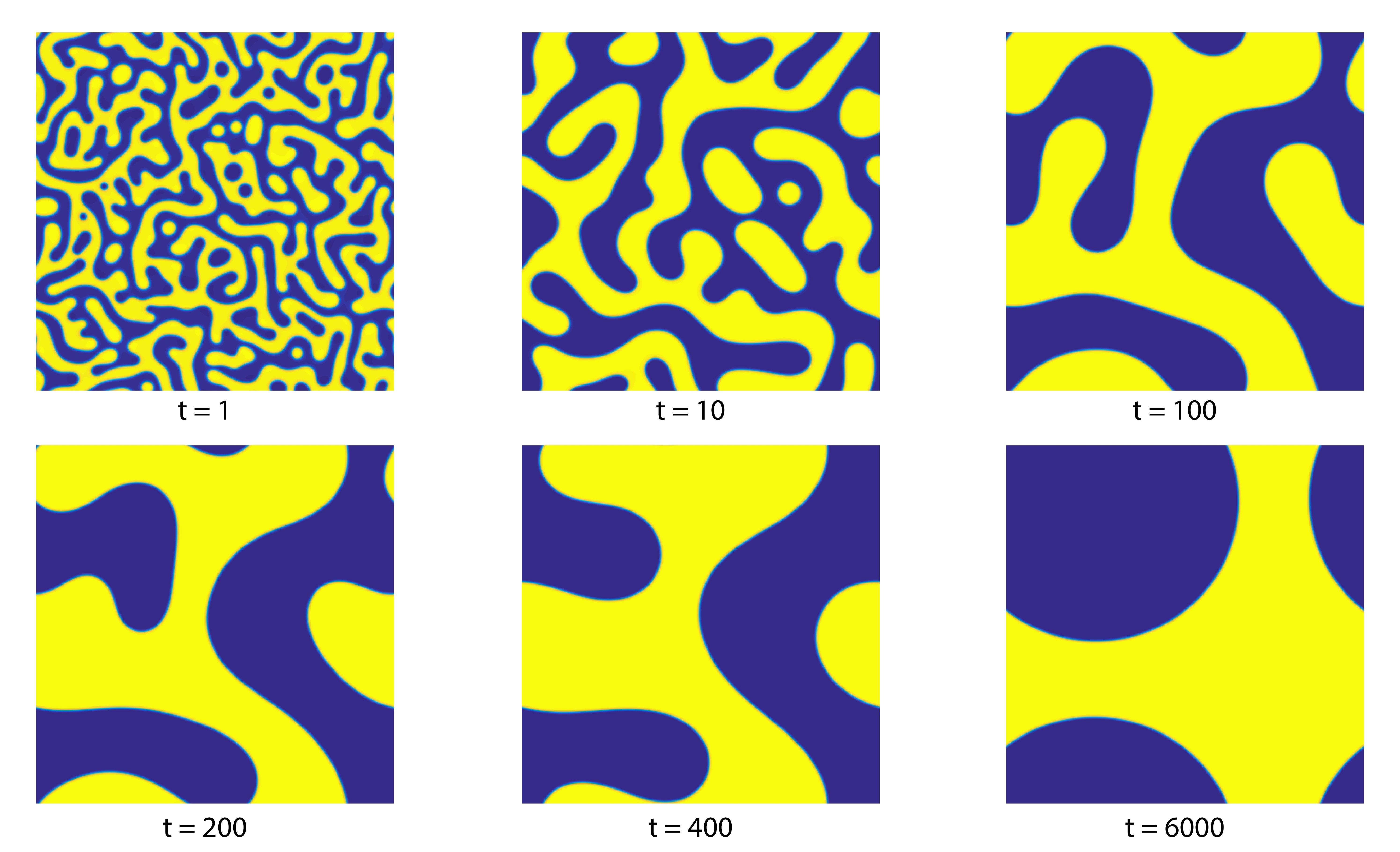
We simulate the spinodal decomposition of a mixed binary fluid and present the energy dissipation in this subsection. The parameters are given by Lx=Ly=12.8L_{x}=L_{y}=12.8, ε=0.03\varepsilon=0.03, h=12.8/512h=12.8/512,. The initial data for this simulation is taken as a random field values ϕi,j0=ϕ¯+0.1⋅(2​ri,j−1)\phi^{0}_{i,j}=\bar{\phi}+0.1\cdot(2r_{i,j}-1), with an average composition ϕ¯=0\bar{\phi}=0 and ri,j∈[0,1]r_{i,j}\in[0,1]. For the temporal step size Δ​t{\Delta t}, we use increasing values of Δ​t{\Delta t} in the time evolution: Δ​t=0.01{\Delta t}=0.01 on the time interval [0,2000][0,2000] and Δ​t=0.04{\Delta t}=0.04 on the time interval [2000,6000][2000,6000]. Whenever a new time step size is applied, we initiate the two-step numerical scheme by taking ϕ−1=ϕ0\phi^{-1}=\phi^{0}, with the initial data ϕ0\phi^{0} given by the final time output of the last time period. The snapshots of spinodal decomposition for the proposed numerical scheme, with second order accuracy in time and fourth order accuracy in space, can be found in Figure 1. The corresponding energy decay plot is displayed in Figure 2.

The log-log plots of energy evolution and the corresponding linear regression in Figure 2 shows that the energy indeed decays like t−1/3t^{-1/3} for the proposed scheme, which verifies the one-third power law. The detailed scaling “exponent” is obtained using least squares fits of the computed data up to time t=400t=400. A clear observation of the ae​t−bea_{e}t^{-b_{e}} scaling law can be made, with ae=2.3670a_{e}=2.3670, be=0.3332b_{e}=0.3332. In other words, an almost perfect t−1/3t^{-1/3} energy dissipation law is confirmed by our numerical simulation.

The linear regressions is only taken up to t=6000t=6000, since the saturation time would be of the order of ε−2\varepsilon^{-2}.

Refer to caption
Figure 1: (Color online). Snapshots of spinodal decomposition of Cahn-Hilliard equation for a mixed binary fluid with scheme (3.9)-(3.10) in Ω=(0,12.8)×(0,12.8)\Omega=(0,12.8)\times(0,12.8) at a sequence of time instants: 1, 10, 100, 200, 400 and 2000. The surface diffusion parameter is taken to be ε=0.03\varepsilon=0.03 and the time step size is Δ​t=0.01{\Delta t}=0.01.
Refer to caption
Figure 2: The evolutions of discrete energy. The parameters are given in the text and in the caption of Figure 1. The energy decays like t−1/3t^{-1/3}, which verifies the one-third power law. More precisely, the linear fit has the form ae​t−bea_{e}t^{-b_{e}} with ae=2.3670,be=−0.3332a_{e}=2.3670,b_{e}=-0.3332.

6 Concluding remarks

In this article, we propose and analyze an energy stable fourth order finite difference scheme for the Cahn-Hilliard equation, with second order temporal accuracy. As a preliminary truncation error estimate for the long stencil difference operator, over a uniform numerical grid with a periodic boundary condition, the discrete ℓ2\ell^{2} estimate only requires an HmH^{m} regularity for the test function, which in turn results in a reduced regularity requirement. In the temporal approximation, we apply a modified BDF algorithm, combined with a second order extrapolation formula applied to the concave term. And also, a second order artificial Douglas-Dupont regularization is included in the numerical scheme, to ensure the energy stability at a discrete level. With such a careful construction, the unique solvability and energy stability are proved for the proposed numerical scheme, and a uniform in time Hh1H_{h}^{1} bound for the numerical solution is established. As a result of this Hh1H_{h}^{1} bound, we are able to derive an optimal rate convergence analysis for the proposed numerical scheme, in the ℓ∞​(0,T,ℓ2)∩ℓ2​(0,T,Hh2)\ell^{\infty}(0,T;\ell^{2})\cap\ell^{2}(0,T;H_{h}^{2}) norm. In addition, a few numerical experiments have confirmed these theoretical results, and the numerical simulations results of spinodal decomposition in a mixed binary fluid have indicated an energy dissipation law of t−1/3t^{-1/3}.

Appendix A Proof of Lemma 2.5

By substituting (2.36), we see that the first inequality of (2.44) is equivalent to

|−4​sin2​(k​π​h/L)−43​sin4​(k​π​h/L)+4​k2​π2​h2L2|≤C1​h6​(2​k​πL)6,∀  0≤k≤N.\left|-4\mbox{sin}^{2}(k\pi h/L)-\frac{4}{3}\mbox{sin}^{4}(k\pi h/L)+\frac{4k^{2}\pi^{2}h^{2}}{L^{2}}\right|\leq C_{1}h^{6}\left(\frac{2k\pi}{L}\right)^{6},\quad\forall\,\,0\leq k\leq N. (A.1)

We denote ck=k​π​h/Lc_{k}=k\pi h/L. Due to the fact that h=L2​N+1h=\frac{L}{2N+1}, we have

0≤ck≤π2,∀  1≤k≤N.0\leq c_{k}\leq\frac{\pi}{2},\quad\forall\,\,1\leq k\leq N. (A.2)

In turn, we need both the lower and upper bounds of −4​sin2​ck−43​sin4​ck+4​ck2-4\mbox{sin}^{2}c_{k}-\frac{4}{3}\mbox{sin}^{4}c_{k}+4c_{k}^{2} to establish the estimate (A.1). For the lower bound, the following inequality is observed:

h1​(t):=sin2​t+13​sin4​t≤h2​(t):=t2,∀t≥0.h_{1}(t):=\mbox{sin}^{2}t+\frac{1}{3}\mbox{sin}^{4}t\leq h_{2}(t):=t^{2},\quad\forall\,\,t\geq 0. (A.3)

The derivation of this inequality is based on the fact that

h1​(0)=h2​(0)=0,h1′​(0)=h2′​(0)=0,h_{1}(0)=h_{2}(0)=0,\quad h^{\prime}_{1}(0)=h^{\prime}_{2}(0)=0, (A.4)

and a careful comparison between their second order derivatives:

h1′′​(t)=2​(cos2​t+sin2​t​cos2​t−53​sin4​t)≤h2′′​(t)=2,∀t≥0.h^{\prime\prime}_{1}(t)=2\left(\mbox{cos}^{2}t+\mbox{sin}^{2}t\mbox{cos}^{2}t-\frac{5}{3}\mbox{sin}^{4}t\right)\leq h^{\prime\prime}_{2}(t)=2,\quad\forall\,\,t\geq 0. (A.5)

As a result of (A.3), we obtain the following lower bound:

0≤−4​sin2​ck−43​sin4​ck+4​ck2,∀  0≤k≤N.0\leq-4\mbox{sin}^{2}c_{k}-\frac{4}{3}\mbox{sin}^{4}c_{k}+4c_{k}^{2},\quad\forall\,\,0\leq k\leq N. (A.6)

For the upper bound, we begin with a Taylor expansion for sin​t\mbox{sin}t:

sin​t≥t−t33!=t−t36≥0,∀  0≤t≤π2,\mbox{sin}t\geq t-\frac{t^{3}}{3!}=t-\frac{t^{3}}{6}\geq 0,\quad\forall\,\,0\leq t\leq\frac{\pi}{2}, (A.7)

in which the second inequality comes from the range that 0≤t≤π20\leq t\leq\frac{\pi}{2}. Subsequently, we set ck=k​π​h/Lc_{k}=k\pi h/L and arrive at

4​sin2​ck+43​sin4​ck≥4​(ck−ck36)2+43​(ck−ck36)4=4​ck2−79​ck6+29​ck8−281​ck10+1972​ck12,\displaystyle 4\mbox{sin}^{2}c_{k}+\frac{4}{3}\mbox{sin}^{4}c_{k}\geq 4\left(c_{k}-\frac{c_{k}^{3}}{6}\right)^{2}+\frac{4}{3}\left(c_{k}-\frac{c_{k}^{3}}{6}\right)^{4}=4c_{k}^{2}-\frac{7}{9}c_{k}^{6}+\frac{2}{9}c_{k}^{8}-\frac{2}{81}c_{k}^{10}+\frac{1}{972}c_{k}^{12}, (A.8)

for any 0≤k≤N0\leq k\leq N. In turn, the following estimate is available:

−4​sin2​ck−43​sin4​ck+4​ck2≤79​ck6−29​ck8+281​ck10−1972​ck12,∀  0≤k≤N.\displaystyle-4\mbox{sin}^{2}c_{k}-\frac{4}{3}\mbox{sin}^{4}c_{k}+4c_{k}^{2}\leq\frac{7}{9}c_{k}^{6}-\frac{2}{9}c_{k}^{8}+\frac{2}{81}c_{k}^{10}-\frac{1}{972}c_{k}^{12},\quad\forall\,\,0\leq k\leq N. (A.9)

Consequently, a combination of (A.6) and (A.9) results in

|−4​sin2​ck−43​sin4​ck+4​ck2|≤79​ck6−29​ck8+281​ck10−1972​ck12,∀  0≤k≤N.\displaystyle\left|-4\mbox{sin}^{2}c_{k}-\frac{4}{3}\mbox{sin}^{4}c_{k}+4c_{k}^{2}\right|\leq\frac{7}{9}c_{k}^{6}-\frac{2}{9}c_{k}^{8}+\frac{2}{81}c_{k}^{10}-\frac{1}{972}c_{k}^{12},\quad\forall\,\,0\leq k\leq N. (A.10)

On the other hand, by the definition ck=k​π​h/Lc_{k}=k\pi h/L, the following estimates can be derived:

ck6=h6​(k​π/L)6≤164​h6​(2​k​π/L)6,∀  0≤k≤N,\displaystyle c_{k}^{6}=h^{6}\left(k\pi/L\right)^{6}\leq\frac{1}{64}h^{6}\left(2k\pi/L\right)^{6},\quad\forall\,\,0\leq k\leq N, (A.11)
ckm=ck6⋅ckm−6≤(π2)m−6⋅164​h6​(2​k​π/L)6,∀m≥6,  0≤k≤N.\displaystyle c_{k}^{m}=c_{k}^{6}\cdot c_{k}^{m-6}\leq\left(\frac{\pi}{2}\right)^{m-6}\cdot\frac{1}{64}h^{6}\left(2k\pi/L\right)^{6},\quad\forall\,\,m\geq 6,\,\,0\leq k\leq N. (A.12)

Finally, a combination of (A.10), (A.11) and (A.12) implies (A.1), with an appropriate choice of C1C_{1}. The proof of the first part of Lemma 2.5 is finished. The second inequality can be derived in the same manner.

Appendix B Proof of Lemma 2.6

We see that the expansion for ‖Δ3​f‖L2\left\|\Delta^{3}f\right\|_{L^{2}} in (2.32) can be decomposed in the following way:

‖Δ3​f‖22=∑k,l=−NNIk,l,with\displaystyle\left\|\Delta^{3}f\right\|_{2}^{2}=\sum_{k,l=-N}^{N}I_{k,l},\quad\mbox{with}
Ik,l=L2​∑k1,l1=−∞∞((2​(k+k1​N∗)​πL)2+(2​(l+l1​N∗)​πL)2)6​|f^k+k1​N∗,l+l1​N∗|2.\displaystyle I_{k,l}=L^{2}\sum_{k_{1},l_{1}=-\infty}^{\infty}\left(\left(\frac{2(k+k_{1}N^{*})\pi}{L}\right)^{2}+\left(\frac{2(l+l_{1}N^{*})\pi}{L}\right)^{2}\right)^{6}\left|\hat{f}_{k+k_{1}N^{*},l+l_{1}N^{*}}\right|^{2}. (B.1)

In particular, we observe that

((2​(k+k1​N∗)​πL)2+(2​(l+l1​N∗)​πL)2)6​|f^k+k1​N∗,l+l1​N∗|2≤Ik,lL2,\displaystyle\left(\left(\frac{2(k+k_{1}N^{*})\pi}{L}\right)^{2}+\left(\frac{2(l+l_{1}N^{*})\pi}{L}\right)^{2}\right)^{6}\left|\hat{f}_{k+k_{1}N^{*},l+l_{1}N^{*}}\right|^{2}\leq\frac{I_{k,l}}{L^{2}},
i.e.|f^k+k1​N∗,l+l1​N∗|≤((2​(k+k1​N∗)​πL)2+(2​(l+l1​N∗)​πL)2)−3​Ik,lL3.\displaystyle\quad\mbox{i.e.}\quad\left|\hat{f}_{k+k_{1}N^{*},l+l_{1}N^{*}}\right|\leq\left(\left(\frac{2(k+k_{1}N^{*})\pi}{L}\right)^{2}+\left(\frac{2(l+l_{1}N^{*})\pi}{L}\right)^{2}\right)^{-3}\sqrt{\frac{I_{k,l}}{L^{3}}}. (B.2)

Meanwhile, the following fact is obvious

|λk​x,(4)+4​(k+k1​N∗)2​π2L2|≤4​(k+k1​N∗)2​π2L2,since λk​x,(4)≤0 and |λk​x,(4)|≤4​k2​π2L2.\left|\lambda_{kx,(4)}+\frac{4(k+k_{1}N^{*})^{2}\pi^{2}}{L^{2}}\right|\leq\frac{4(k+k_{1}N^{*})^{2}\pi^{2}}{L^{2}},\quad\mbox{since $\lambda_{kx,(4)}\leq 0$ and $|\lambda_{kx,(4)}|\leq\frac{4k^{2}\pi^{2}}{L^{2}}$}. (B.3)

Therefore, the following estimate is valid for a fixed (k,l)(k,l) and (k1,l1)≠(0,0)(k_{1},l_{1})\neq(0,0):

|(λk​x,(4)+4​(k+k1​N∗)2​π2L2)​f^k+k1​N∗,l+l1​N∗|≤4​(k+k1​N∗)2​π2L2​|f^k+k1​N∗,l+l1​N∗|\displaystyle\hskip-54.2025pt\left|\left(\lambda_{kx,(4)}+\frac{4(k+k_{1}N^{*})^{2}\pi^{2}}{L^{2}}\right)\hat{f}_{k+k_{1}N^{*},l+l_{1}N^{*}}\right|\leq\frac{4(k+k_{1}N^{*})^{2}\pi^{2}}{L^{2}}\left|\hat{f}_{k+k_{1}N^{*},l+l_{1}N^{*}}\right| (B.4)
≤\displaystyle\leq ((2​(k+k1​N∗)​πL)2+(2​(l+l1​N∗)​πL)2)−2​Ik,lL2\displaystyle\left(\left(\frac{2(k+k_{1}N^{*})\pi}{L}\right)^{2}+\left(\frac{2(l+l_{1}N^{*})\pi}{L}\right)^{2}\right)^{-2}\sqrt{\frac{I_{k,l}}{L^{2}}}
≤\displaystyle\leq (4​(N∗)2​π2L2​((|k1|−12)2+(|l1|−12)2))−2​Ik,lL2\displaystyle\left(\frac{4(N^{*})^{2}\pi^{2}}{L^{2}}\left((|k_{1}|-\frac{1}{2})^{2}+(|l_{1}|-\frac{1}{2})^{2}\right)\right)^{-2}\sqrt{\frac{I_{k,l}}{L^{2}}}
≤\displaystyle\leq 116​h4​π−4​Ik,lL2​1((|k1|−12)2+(|l1|−12)2)2,\displaystyle\frac{1}{16}h^{4}\pi^{-4}\sqrt{\frac{I_{k,l}}{L^{2}}}\frac{1}{\left((|k_{1}|-\frac{1}{2})^{2}+(|l_{1}|-\frac{1}{2})^{2}\right)^{2}},

in which the grid size h=L2​N+1h=\frac{L}{2N+1} was recalled. Also note that we used the following estimate in the third step

|k+k1N∗|≥(|k1|−12)​N∗2,|l+l1N∗|≥(|l1|−12)​N∗2,fork1≠0,l1≠0,\left|k+k_{1}N^{*}\right|\geq\frac{(|k_{1}|-\frac{1}{2})N^{*}}{2},\quad\left|l+l_{1}N^{*}\right|\geq\frac{(|l_{1}|-\frac{1}{2})N^{*}}{2},\quad\mbox{for}\quad k_{1}\neq 0,\,\,l_{1}\neq 0, (B.5)

due to the fact that |k|,|l|≤N∗/2|k|,|l|\leq N^{*}/2. Consequently, its substitution into (2.45) shows that

|∑k1,l1=−∞(k1,l1)≠(0,0)∞(λk​x,(4)+4​(k+k1​N∗)2​π2L2)​f^k+k1​N∗,l+l1​N∗|\displaystyle\hskip-36.135pt\left|\sum_{k_{1},l_{1}=-\infty\atop(k_{1},l_{1})\neq(0,0)}^{\infty}\left(\lambda_{kx,(4)}+\frac{4(k+k_{1}N^{*})^{2}\pi^{2}}{L^{2}}\right)\hat{f}_{k+k_{1}N^{*},l+l_{1}N^{*}}\right| (B.6)
≤\displaystyle\leq ∑k1,l1=−∞(k1,l1)≠(0,0)∞|(λk​x,(4)+4​(k+k1​N∗)2​π2L2)​f^k+k1​N∗,l+l1​N∗|\displaystyle\sum_{k_{1},l_{1}=-\infty\atop(k_{1},l_{1})\neq(0,0)}^{\infty}\left|\left(\lambda_{kx,(4)}+\frac{4(k+k_{1}N^{*})^{2}\pi^{2}}{L^{2}}\right)\hat{f}_{k+k_{1}N^{*},l+l_{1}N^{*}}\right|
≤\displaystyle\leq ∑k1,l1=−∞(k1,l1)≠(0,0)∞116​h4​π−4​Ik,lL2​1((|k1|−12)2+(|l1|−12)2)2=C∗​h4​Ik,lL2,\displaystyle\sum_{k_{1},l_{1}=-\infty\atop(k_{1},l_{1})\neq(0,0)}^{\infty}\frac{1}{16}h^{4}\pi^{-4}\sqrt{\frac{I_{k,l}}{L^{2}}}\frac{1}{\left((|k_{1}|-\frac{1}{2})^{2}+(|l_{1}|-\frac{1}{2})^{2}\right)^{2}}=C^{*}h^{4}\sqrt{\frac{I_{k,l}}{L^{2}}},

where

C∗=116​π−4​∑k1,l1=−∞(k1,l1)≠(0,0)∞1((|k1|−12)2+(|l1|−12)2)2.C^{*}=\frac{1}{16}\pi^{-4}\sum_{k_{1},l_{1}=-\infty\atop(k_{1},l_{1})\neq(0,0)}^{\infty}\frac{1}{\left((|k_{1}|-\frac{1}{2})^{2}+(|l_{1}|-\frac{1}{2})^{2}\right)^{2}}. (B.7)

Note that the double series

∑k1,l1=−∞(k1,l1)≠(0,0)∞1((|k1|−12)2+(|l1|−12)2)β0,\sum_{k_{1},l_{1}=-\infty\atop(k_{1},l_{1})\neq(0,0)}^{\infty}\frac{1}{\left((|k_{1}|-\frac{1}{2})^{2}+(|l_{1}|-\frac{1}{2})^{2}\right)^{\beta_{0}}}, (B.8)

with β0=2\beta_{0}=2, is convergent. In turn, we arrive at

∑k,l=−NN|∑k1,l1=−∞(k1,l1)≠(0,0)∞(λk​x,(4)+4​(k+k1​N∗)2​π2L2)​f^k+k1​N∗,l+l1​N∗|2\displaystyle\hskip-36.135pt\sum_{k,l=-N}^{N}\left|\sum_{k_{1},l_{1}=-\infty\atop(k_{1},l_{1})\neq(0,0)}^{\infty}\left(\lambda_{kx,(4)}+\frac{4(k+k_{1}N^{*})^{2}\pi^{2}}{L^{2}}\right)\hat{f}_{k+k_{1}N^{*},l+l_{1}N^{*}}\right|^{2} (B.9)
≤\displaystyle\leq ∑k,l=−NN(C∗)2​h8⋅Ik,lL2=(C∗)2L2​h8​∑k,l=−NNIk,l=(C∗)2L2​h8​‖Δ3​f‖2\displaystyle\sum_{k,l=-N}^{N}(C^{*})^{2}h^{8}\cdot\frac{I_{k,l}}{L^{2}}=\frac{(C^{*})^{2}}{L^{2}}h^{8}\sum_{k,l=-N}^{N}I_{k,l}=\frac{(C^{*})^{2}}{L^{2}}h^{8}\left\|\Delta^{3}f\right\|^{2}
=\displaystyle= (C∗)2L2​h8​‖f‖H62,\displaystyle\frac{(C^{*})^{2}}{L^{2}}h^{8}\left\|f\right\|_{H^{6}}^{2},

in which the decomposition (B.1) was used in the second to the last step. Therefore, the first inequality of Lemma 2.6 is proven by taking C2=(C∗)2L2C_{2}=\frac{(C^{*})^{2}}{L^{2}}. The second inequality of Lemma 2.6 can be established in the same manner. This completes the proof of Lemma 2.6.

Appendix C Proof of Lemma 3.2

Proof.

For any periodic grid function ff, it has a corresponding discrete Fourier transformation:

fi,j\displaystyle f_{i,j} =\displaystyle= ∑ℓ,m=−NNf^ℓ,mN​e2​π​i​(ℓ​xi+m​yj)/L,\displaystyle\sum^{N}_{\ell,m=-N}\hat{f}^{N}_{\ell,m}{\rm e}^{2\pi i(\ell x_{i}+my_{j})/L}, (C.1)

where xi=(i−12)​hx_{i}=(i-\frac{1}{2})h, yj=(j−12)​hy_{j}=(j-\frac{1}{2})h, and f^ℓ,mN\hat{f}^{N}_{\ell,m} are the coefficients. In turn, for an application of the operator −Δh,(4)-\Delta_{h,(4)} to ff, the following discrete Fourier expansion is available:

−Δh​fi,j=∑ℓ,m=−NN(νℓ+νm)​f^ℓ,mN​e2​π​i​(ℓ​xi+m​yj)/L,\displaystyle-\Delta_{h}f_{i,j}=\sum^{N}_{\ell,m=-N}(\nu_{\ell}+\nu_{m})\hat{f}^{N}_{\ell,m}{\rm e}^{2\pi i(\ell x_{i}+my_{j})/L}, (C.2)
−Δh,(4)​fi,j=∑ℓ,m=−NNΛℓ,m​f^ℓ,mN​e2​π​i​(ℓ​xi+m​yj)/L,\displaystyle-\Delta_{h,(4)}f_{i,j}=\sum^{N}_{\ell,m=-N}\Lambda_{\ell,m}\hat{f}^{N}_{\ell,m}{\rm e}^{2\pi i(\ell x_{i}+my_{j})/L}, (C.3)
with​νk=4​sin2⁡ℓ​π​hLh2,μk=νk2+h212​νk2,Λℓ,m=μℓ+μm.\displaystyle\mbox{with}\,\,\nu_{k}=\frac{4\sin^{2}{\frac{\ell\pi h}{L}}}{h^{2}},\,\,\mu_{k}=\nu_{k}^{2}+\frac{h^{2}}{12}\nu_{k}^{2},\,\,\Lambda_{\ell,m}=\mu_{\ell}+\mu_{m}. (C.4)

For any f∈𝒱̊perf\in\mathring{\cal V}_{\rm per}, we observe that h​a​t​fℓ,mN=0hat{f}^{N}_{\ell,m}=0, due to the fact that f¯=0\overline{f}=0. In turn, a similar expansion could be derived for (−Δh,(4))−1​f(-\Delta_{h,(4)})^{-1}f:

(−Δh,(4))−1​fi,j=∑ℓ,m≠(0,0)Λℓ,m−1​f^ℓ,mN​e2​π​i​(ℓ​xi+m​yj)/L.\displaystyle(-\Delta_{h,(4)})^{-1}f_{i,j}=\sum_{\ell,m\neq(0,0)}\Lambda_{\ell,m}^{-1}\hat{f}^{N}_{\ell,m}{\rm e}^{2\pi i(\ell x_{i}+my_{j})/L}. (C.5)

On the other hand, the following identities could be derived, based on the orthonormal property of the Fourier basis function:

∥∥f∥−1,h2=(f,(−Δh,(4))−1f)2=L2∑ℓ,m≠(0,0)Λℓ,m−1|f^ℓ,mN|2,\displaystyle\|\|f\|_{-1,h}^{2}=(f,(-\Delta_{h,(4)})^{-1}f)_{2}=L^{2}\sum_{\ell,m\neq(0,0)}\Lambda_{\ell,m}^{-1}|\hat{f}^{N}_{\ell,m}|^{2}, (C.6)
‖∇h,(4)f‖22=(f,−Δh,(4)​f)2=L2​∑ℓ,m≠(0,0)Λℓ,m​|f^ℓ,mN|2,\displaystyle\|\nabla_{h,(4)}f\|_{2}^{2}=(f,-\Delta_{h,(4)}f)_{2}=L^{2}\sum_{\ell,m\neq(0,0)}\Lambda_{\ell,m}|\hat{f}^{N}_{\ell,m}|^{2}, (C.7)

for any f∈𝒱̊perf\in\mathring{\cal V}_{\rm per}. Meanwhile, an application of Parseval equality to (C.1) implies that

∥∥f∥2=L2∑ℓ,m≠(0,0)|f^Nℓ,m|2.\displaystyle\|\|f\|^{2}=L^{2}\sum_{\ell,m\neq(0,0)}|\hat{f}^{N}_{\ell,m}|^{2}. (C.8)

An application of discrete Cauchy-Schwarz inequality leads to

(∑ℓ,m≠(0,0)|f^ℓ,mN|2)2≤(∑ℓ,m≠(0,0)Λℓ,m−1​|f^ℓ,mN|2)⋅(∑ℓ,m≠(0,0)Λℓ,m​|f^ℓ,mN|2),\displaystyle\left(\sum_{\ell,m\neq(0,0)}|\hat{f}^{N}_{\ell,m}|^{2}\right)^{2}\leq\left(\sum_{\ell,m\neq(0,0)}\Lambda_{\ell,m}^{-1}|\hat{f}^{N}_{\ell,m}|^{2}\right)\cdot\left(\sum_{\ell,m\neq(0,0)}\Lambda_{\ell,m}|\hat{f}^{N}_{\ell,m}|^{2}\right), (C.9)

which is equivalent to ‖f‖24≤‖f‖−1,h2⋅‖∇h,(4)f‖22\|f\|_{2}^{4}\leq\|f\|_{-1,h}^{2}\cdot\|\nabla_{h,(4)}f\|_{2}^{2}, for any f∈𝒱̊perf\in\mathring{\cal V}_{\rm per}. This completes the proof of (3.7).

The proof of (3.8) follows a similar argument. By making a comparison between (C.2) and (C.3), combined with an application of Parseval equality, we get

‖Δh​f‖22=L2​∑ℓ,m=−NN(νℓ+νm)2​|f^ℓ,mN|2,\displaystyle\|\Delta_{h}f\|_{2}^{2}=L^{2}\sum^{N}_{\ell,m=-N}(\nu_{\ell}+\nu_{m})^{2}|\hat{f}^{N}_{\ell,m}|^{2}, (C.10)
‖Δh,(4)​f‖2=L2​∑ℓ,m=−NNΛℓ,m2​|f^ℓ,mN|2.\displaystyle\|\Delta_{h,(4)}f\|_{2}=L^{2}\sum^{N}_{\ell,m=-N}\Lambda_{\ell,m}^{2}|\hat{f}^{N}_{\ell,m}|^{2}. (C.11)

Therefore, (3.8) becomes a direct consequence of the following fact:

|νℓ+νm|=νℓ+νm≤Λℓ,m=|Λℓ,m|.\displaystyle|\nu_{\ell}+\nu_{m}|=\nu_{\ell}+\nu_{m}\leq\Lambda_{\ell,m}=|\Lambda_{\ell,m}|. (C.12)

The proof of Lemma 3.2 is finished. ∎

Acknowledgements

This work is supported in part by the grants NSF DMS-1418689 (C. Wang), NSF DMS-1418692 and NSF DMS-1719854 (S. Wise).

References

  • [1] J. Barrett and J. Blowey. Finite element approximation of the Cahn-Hilliard equation with concentration dependent mobility. Math. Comp., 68:487–517, 1999.
  • [2] A. Baskaran, Z. Hu, J. Lowengrub, C. Wang, S.M. Wise, and P. Zhou. Energy stable and efficient finite-difference nonlinear multigrid schemes for the modified phase field crystal equation. J. Comput. Phys., 250:270–292, 2013.
  • [3] A. Baskaran, J. Lowengrub, C. Wang, and S. Wise. Convergence analysis of a second order convex splitting scheme for the modified phase field crystal equation. SIAM J. Numer. Anal., 51:2851–2873, 2013.
  • [4] J.P. Boyd. Chebyshev and Fourier spectral methods. Courier Corporation, 2001.
  • [5] J.W. Cahn and J.E. Hilliard. Free energy of a nonuniform system. i. interfacial free energy. J. Chem. Phys., 28:258–267, 1958.
  • [6] C. Canuto and A. Quarteroni. Approximation results for orthogonal polynomials in Sobolev spaces. Math. Comp., 38:67–86, 1982.
  • [7] W. Chen, S. Conde, C. Wang, X. Wang, and S.M. Wise. A linear energy stable scheme for a thin film model without slope selection. J. Sci. Comput., 52:546–562, 2012.
  • [8] W. Chen, Y. Liu, C. Wang, and S.M. Wise. An optimal-rate convergence analysis of a fully discrete finite difference scheme for Cahn-Hilliard-Hele-Shaw equation. Math. Comp., 85:2231–2257, 2016.
  • [9] W. Chen, C. Wang, X. Wang, and S.M. Wise. A linear iteration algorithm for energy stable second order scheme for a thin film model without slope selection. J. Sci. Comput., 59:574–601, 2014.
  • [10] K. Cheng, W. Feng, S. Gottlieb, and C. Wang. A Fourier pseudospectral method for the “Good” Boussinesq equation with second-order temporal accuracy. Numer. Methods Partial Differential Equations, 31(1):202–224, 2015.
  • [11] K. Cheng, C. Wang, S.M. Wise, and X. Yue. A second-order, weakly energy-stable pseudo-spectral scheme for the Cahn-Hilliard equation and its solution by the homogeneous linear iteration method. J. Sci. Comput., 69:1083–1114, 2016.
  • [12] A. Diegel, X. Feng, and S.M. Wise. Convergence analysis of an unconditionally stable method for a Cahn-Hilliard-Stokes system of equations. SIAM J. Numer. Anal., 53:127–152, 2015.
  • [13] A. Diegel, C. Wang, X. Wang, and S.M. Wise. Convergence analysis and error estimates for a second order accurate finite element method for the Cahn-Hilliard-Navier-Stokes system. Numer. Math., 137:495–534, 2017.
  • [14] A. Diegel, C. Wang, and S.M. Wise. Stability and convergence of a second order mixed finite element method for the Cahn-Hilliard equation. IMA J. Numer. Anal., 36:1867–1897, 2016.
  • [15] Q. Du and R. Nicolaides. Numerical analysis of a continuum model of a phase transition. SIAM J. Numer. Anal., 28:1310–1322, 1991.
  • [16] C.M. Elliott, D.A French, and F.A. Milner. A second-order splitting method for the Cahn-Hilliard equation. Numer. Math., 54:575–590, 1989.
  • [17] C.M. Elliott and A.M. Stuart. The global dynamics of discrete semilinear parabolic equations. SIAM J. Numer. Anal., 30:1622–1663, 1993.
  • [18] D. Eyre. Unconditionally gradient stable time marching the Cahn-Hilliard equation. In J. W. Bullard, R. Kalia, M. Stoneham, and L.Q. Chen, editors, Computational and Mathematical Models of Microstructural Evolution, volume 53, pages 1686–1712, Warrendale, PA, USA, 1998. Materials Research Society.
  • [19] A. Fathy, C. Wang, J. Wilson, and S. Yang. A fourth order difference scheme for the maxwell equations on yee grid. J. Hyperbol. Differ. Eq., 5(03):613–642, 2008.
  • [20] W. Feng, A.J. Salgado, C. Wang, and S.M. Wise. Preconditioned steepest descent methods for some nonlinear elliptic equations involving p-Laplacian terms. J. Comput. Phys., 334:45–67, 2017.
  • [21] W. Feng, C. Wang, S.M. Wise, and Z. Zhang. A second-order energy stable Backward Differentiation Formula method for the epitaxial thin film equation with slope selection. Numer. Methods Partial Differ. Equ., 2017. Submitted and in review.
  • [22] X. Feng and A. Prohl. Error analysis of a mixed finite element method for the Cahn-Hilliard equation. Numer. Math., 99:47–84, 2004.
  • [23] X. Feng and S.M. Wise. Analysis of a fully discrete finite element approximation of a Darcy-Cahn-Hilliard diffuse interface model for the Hele-Shaw flow. SIAM J. Numer. Anal., 50:1320–1343, 2012.
  • [24] B. Fornberg. Generation of finite difference formulas on arbitrarily spaced grids. Math. Comp., 51(184):699–706, 1988.
  • [25] B. Fornberg. Classroom note: Calculation of weights in finite difference formulas. SIAM review, 40(3):685–691, 1998.
  • [26] D. Furihata. A stable and conservative finite difference scheme for the Cahn-Hilliard equation. Numer. Math., 87:675–699, 2001.
  • [27] D. Gottlieb and S. A. Orszag. Numerical analysis of spectral methods: theory and applications. SIAM, 1983.
  • [28] Z. Guan, J.S. Lowengrub, C. Wang, and S.M. Wise. Second-order convex splitting schemes for nonlocal Cahn-Hilliard and Allen-Cahn equations. J. Comput. Phys., 277:48–71, 2014.
  • [29] Z. Guan, C. Wang, and S.M. Wise. A convergent convex splitting scheme for the periodic nonlocal Cahn-Hilliard equation. Numer. Math., 128:377–406, 2014.
  • [30] J. Guo, C. Wang, S.M. Wise, and X. Yue. An H2H^{2} convergence of a second-order convex-splitting, finite difference scheme for the three-dimensional Cahn-Hilliard equation. Commu. Math. Sci., 14:489–515, 2016.
  • [31] D. Han and X. Wang. A second order in time, uniquely solvable, unconditionally stable numerical scheme for Cahn-Hilliard-Navier-Stokes equation. J. Comput. Phys., 290:139–156, 2015.
  • [32] Y. He, Y. Liu, and T. Tang. On large time-stepping methods for the Cahn-Hilliard equation. Appl. Numer. Math., 57(4):616–628, 2006.
  • [33] J. S. Hesthaven, S. Gottlieb, and D. Gottlieb. Spectral methods for time-dependent problems, volume 21. Cambridge University Press, 2007.
  • [34] Z. Hu, S. Wise, C. Wang, and J. Lowengrub. Stable and efficient finite-difference nonlinear-multigrid schemes for the phase-field crystal equation. J. Comput. Phys., 228:5323–5339, 2009.
  • [35] A. Iserles. A first course in the numerical analysis of differential equations, volume 44. Cambridge University Press, 2009.
  • [36] D. Kay and R. Welford. A multigrid finite element solver for the Cahn-Hilliard equation. J. Comput. Phys., 212:288–304, 2006.
  • [37] D. Kay and R. Welford. Efficient numerical solution of Cahn-Hilliard-Navier-Stokes fluids in 2D. SIAM J. Sci. Comput., 29:2241–2257, 2007.
  • [38] N. Khiari, T. Achouri, M.L. Ben Mohamed, and K. Omrani. Finite difference approximate solutions for the Cahn-Hilliard equation. Numer. Meth. PDE, 23:437–455, 2007.
  • [39] J.S. Kim, K. Kang, and J.S. Lowengrub. Conservative multigrid methods for Cahn-Hilliard fluids. J. Comput. Phys., 193:511–543, 2003.
  • [40] C. Lee, D. Jeong, J. Shin, Y. Li, and J. Kim. A fourth-order spatial accurate and practically stable compact scheme for the Cahn-Hilliard equation. Physica A, 409:17–28, 2014.
  • [41] D. Li and Z. Qiao. On second order semi-implicit Fourier spectral methods for 2D Cahn-Hilliard equations. J. Sci. Comput., 70:301–341, 2017.
  • [42] J. Li, Z. Sun, and X. Zhao. A three level linearized compact difference scheme for the Cahn-Hilliard equation. Sci. China Math., 55:805–826, 2012.
  • [43] Y. Li, H. Lee, B. Xia, and J. Kim. A compact fourth-order finite difference scheme for the three-dimensional Cahn-Hilliard equation. Comput. Phys. Commun., 200:108–116, 2016.
  • [44] J.-G. Liu and C. Wang. A fourth order numerical method for the primitive equations formulated in mean vorticity. Commun. Comput. Phys, 4:26–55, 2008.
  • [45] J.-G. Liu, C. Wang, and H. Johnston. A fourth order scheme for incompressible Boussinesq equations. J. Sci. Comput., 18(2):253–285, 2003.
  • [46] Y. Liu, W. Chen, C. Wang, and S.M. Wise. Error analysis of a mixed finite element method for a Cahn-Hilliard-Hele-Shaw system. Numer. Math., 135:679–709, 2017.
  • [47] S.A. Orszag and C.M. Bender. Advanced mathematical methods for scientists and engineers. Mac Graw Hill, 1978.
  • [48] R. Samelson, R. Temam, C. Wang, and S. Wang. A fourth-order numerical method for the planetary geostrophic equations with inviscid geostrophic balance. Numer. Math., 107(4):669–705, 2007.
  • [49] J. Shen, C. Wang, X. Wang, and S.M. Wise. Second-order convex splitting schemes for gradient flows with Ehrlich-Schwoebel type energy: Application to thin film epitaxy. SIAM J. Numer. Anal., 50:105–125, 2012.
  • [50] H. Song. Energy stable and large time-stepping methods for the Cahn-Hilliard equation. Inter. J. Comput. Math., 92:2091–2108, 2015.
  • [51] E. Tadmor. The exponential accuracy of fourier and chebyshev differencing methods. SIAM J. Numer. Anal., 23:1–10, 1986.
  • [52] C. Wang, J.-G. Liu, and H. Johnston. Analysis of a fourth order finite difference method for the incompressible Boussinesq equations. Numer. Math., 97(3):555–594, 2004.
  • [53] C. Wang, X. Wang, and S.M. Wise. Unconditionally stable schemes for equations of thin film epitaxy. Discrete Contin. Dyn. Sys. A, 28:405–423, 2010.
  • [54] C. Wang and S.M. Wise. An energy stable and convergent finite-difference scheme for the modified phase field crystal equation. SIAM J. Numer. Anal., 49:945–969, 2011.
  • [55] T. Wang, L. Zhao, and B. Guo. A class of stable and conservative finite difference schemes for the Cahn-Hilliard equation. Acta Math. Appl. Sin. Engl. Ser., 31:863–878, 2015.
  • [56] S.M. Wise. Unconditionally stable finite difference, nonlinear multigrid simulation of the Cahn-Hilliard-Hele-Shaw system of equations. J. Sci. Comput., 44:38–68, 2010.
  • [57] S.M. Wise, J.S. Kim, and J.S. Lowengrub. Solving the regularized, strongly anisotropic Chan-Hilliard equation by an adaptive nonlinear multigrid method. J. Comput. Phys., 226:414–446, 2007.
  • [58] S.M. Wise, C. Wang, and J.S. Lowengrub. An energy stable and convergent finite-difference scheme for the phase field crystal equation. SIAM J. Numer. Anal., 47:2269–2288, 2009.
  • [59] Y. Yan, W. Chen, C. Wang, and S.M. Wise. A second-order energy stable BDF numerical scheme for the Cahn-Hilliard equation. Commun. Comput. Phys., 23:572–602, 2018.