The Crush-Down Equation
for Non-Constant Velocity ProfilesThanks: ansgar.schneider@uni-muenster.de

On the 11th of September 2001 both of the Twin Towers of the World Trade Center in New York City were struck by an aircraft. The North Tower collapsed approximately one and a half hour after the aircraft impact, the South Tower approximately one hour after the aircraft impact. Both buildings collapsed rapidly in a top to down manner.

The National Institute of Standards and Technology released a report in 2005 whose objective was to explain how the collapse of the towers initiated [NIST]. However, they did not even try to explain how the collapse progressed.

Two years later, in 2007, a model was proposed by Bažant and Verdure to describe the gravity-driven collapse of a tall building as a progressive floor collapse [BaVe07]. The heart of this model is the so-called Crush-Down Equation that describes the downward movement of the crushing front of the collapsing building. Another year later Bažant, Benson, Greening and Le modified this model slightly [BLGB08].

In this paper we shall not be concerned about what can be learned from the model when empirical data of the actual collapsing buildings is taken into account. This is done elsewhere [Schn17b]. This paper is solely focused on the modifications that are made on the Crush-Down Equation in [BLGB08].

Let us introduce some notation and the Crush-Down Equation of [BaVe07].

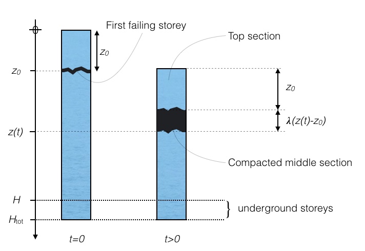
Consider a tall 1-dimensional building whose roof has an elevation of $H$ over concourse level (cp. Figure 1). The total height of the building including its underground storeys will be denoted by $H_{\rm tot}\geq H$. We fix a coordinate system which is pointing downwards to the ground and whose origin has a fixed elevation above concourse level, namely the elevation of the initial undestroyed tower top $H$.

Assume one storey of the building fails due to some extraordinary circumstances at the position $z_{0}>0$ below the tower top, i. e. on the interval $[z_{0},z_{0}+h]$ the column strength is reduced, where $h$ is the height of one storey. The value of $z_{0}$ is the height of the top section of the building that will now decent and destroy the building below it. The destruction of the top section itself can be neglected. An argument for this assumption is given in [BLGB08, Appendix], where a two-sided front propagation is computed. The upward running front of destruction terminates within a fraction of a second after having propagated a couple of centimetres only.

Of course, we assume here that the dynamical load of the impacting top section is sufficiently big such that the collapse will indeed progress. A sufficient condition for the termination of the collapse is given in [BaZh02]. The estimate therin, however, is not optimal in the sense that a weaker condition already suffices to arrest the collapse [Schn17a].

The crushing front will run downwards and we denote the position of the crushing front at time $t$ by $z(t)\geq z_{0}$. Time starts at collapse initiation, so $z(0)=z_{0}$.

We model the collapsing building by three distinct parts which are: 1. The initial top section of mass $m_{0}$ that sat above the first failing floor. This section keeps its height $z_{0}$ until the crushing front hits the ground. 2. The section below the top section which is compacted from its original undamaged size and moving with the same velocity as the top section. The height and mass of this section is growing in time. 3. The resting, still undamaged section below these two. The height of this section at time $t$ is $H-z(t)$. It is reducing while the collapse proceeds.

We assume that during the collapse some fraction of material is spit outwards at the crushing front. We denote this quantity by $\kappa_{\rm out}\in[0,1]$. A value of $\kappa_{\rm out}=0$ is used in [BaVe07], $\kappa_{\rm out}=0.2$ in [BLGB08] and $\kappa_{\rm out}=0.25$ in [Schn17b].

Let us first assume all storeys are compacted to the same height after the crushing front has passed by. We describe this by the so-called compaction parameter $\lambda\in(0,1)$, i. e. if $\Delta z(t):=z(t)-z_{0}$ is the height of the part of the building that has been crushed already, then $\lambda\cdot\Delta z(t)$ is the height of the compacted section at time $t$.

The position of the roof top at time $t$ is $z(t)-\lambda\Delta z(t)-z_{0}=(1-\lambda)\Delta z(t)$, and its time derivative $(1-\lambda)\dot{z}(t)$ is the downward velocity of both the top and the middle section. Therefore the total momentum of the falling two sections at time $t$ is given by

where

is the mass of the compacted section. $\mu(\cdot)$ is the mass height-density of the undestroyed tower. We will assume that $\mu$ is a strictly positive, monotonously increasing, convex continuous function. In particular, it follows that the mass function $\Delta m(\cdot)$ is also convex. Most of our theory can be done for general $\mu$, but later we shall restrict ourselves to the case of the World Trade Center.

Now, the equation of motion—which is called Crush-Down Equation in [BaVe07]— that is valid until the crushing front reaches the ground is given by

where $F(\cdot)>0$ is the upward resistance force due to column buckling, and $g$ is the acceleration of gravity.

Other (velocity dependent) forces can be added to $F$, but we shall not be concerned about this issue here. A discussion of the three terms that are added in [BLGB08] is given in [Schn17b, Section 1.4]. In this paper we shall discuss the question how the total momentum $p(t)$ changes, when two assumptions are altered. These are:

• $(a)$

  The assumption that all storeys get compacted to the same height when the crushing front passes by.

• $(b)$

  The assumption that the compacted section has a trivial (constant) velocity profile.

In [BLGB08] these two points are handled in the following way:

• $(a)$

  Instead of assuming that every storey is compacted to the same height, it is assumed that every storey is compacted to the same density. This means that instead of $\lambda\in(0,1)$ a function $\lambda:[z_{0},H_{\rm tot}]\to(0,1)$ is considered such that $\lambda$ is proportional to $\mu$. This assumption simplifies the analysis significantly as we shall see, but it is not clear at all that this assumption is more realistic than the first one. It seems reasonable to expect that during the collapse the lower storeys get compacted to a higher density than the storeys above. A constant compaction parameter captures at least a glimpse of this aspect.

  We shall consider both cases $\lambda=const$ and $\lambda\sim\mu$ in what follows. Note that these two cases coincide if $\mu(\cdot)$ is constant itself.

• $(b)$

  The velocity profile of the middle section is supposed to vary linearly from the top of the middle section down to the crushing front. However, this modification is not done accurately in [BLGB08] for the following reasons:

  1. $(i)$

     If the velocity profile is non-trivial, then conservation of mass implies that the density of the compacted section is also varying. Yet in [BLGB08] it is assumed that the density is constant.

  2. $(ii)$

     The linear velocity profile of [BLGB08] is assumed to vary between the velocity of the top section (at the top of the compacted layer) and the velocity of the crushing front (at the bottom of the compacted layer). This is an extremely unphysical assumption, because the latter velocity is bigger than the first one. Realistically, the velocity at the bottom of the compacted layer is lower than the velocity at the top. The velocity of the crushing front should not be regarded as the velocity of any mass-bearing instance, but as a quantity that describes the change of the geometry of the crushing building.

The formula for the total momentum that is derived from these erroneous assumptions is formula (2) in [BLGB08]. It can be written as

Note that the second velocity term $(1-\frac{1}{2}\lambda(z))\,\dot{z}$ is just the mean of $\dot{z}$ and $(1-\lambda(z))\dot{z}$, i. e. that’s the average velocity of the linear linear velocity profile.

Let us denote by $y(t)$ the position of the top of the middle section at time $t$. If $z(t)$ is the position of the crushing front at time $t$, the compacted layer has an extension of $\Lambda(t):=z(t)-y(t)$. In particular $\Lambda(0)=0$. We shall derive a relation between $\Lambda$ and the compaction parameter $\lambda:[z_{0},H]\to(0,1)$. $\lambda(z(t))$ describes how much the storeys are compacted at the crushing front $z(t)$. For the two cases $\lambda=const$ and $\lambda\sim\mu$ the theory which we develop is manageable. To clarify our notation we shall use the convention $\lambda(z)=\lambda_{0}$ if $\lambda$ is a constant function, $\lambda_{0}\in\mathbb{R}$. If $\lambda\sim\mu$, we will use the convention $\lambda(z)=\lambda_{0}\frac{\mu(z)}{\mu_{0}}$, where $\mu_{0}:=\mu(z_{0})$.

By $a$ we denote the distance from $y(t)$ to some point $y(t)+a$ in the compacted section, $a\in[0,\Lambda(t)]$. Let us now assume a non-trivial velocity profile $(a,t)\mapsto v(a,t)$. $v(a,t)$ is the difference of $\dot{y}(t)$ and the velocity of the falling part at position $y(t)+a$ at time $t$. So the downward velocity of the falling section at position $y(t)+a$ and time $t$ is given by $\dot{y}(t)+v(a,t)$. In particular $v(0,t)=0$. If $v(a,t)=0$ for all $(a,t)$ we are in the situation as discussed before. The assumption of a linear velocity profile as done in [BLGB08] that reaches the velocity $\dot{z}(t)$ at at the crushing front means that the formula

holds. In fact, in that case $\dot{y}(t)+v(\Lambda(t),t)=\dot{y}(t)+\dot{\Lambda}(t)=\dot{z}(t)$. Let us now more generally assume that the velocity profile is of the form

for $\eta\in\mathbb{R}$ and $w:[0,1]\to[0,\infty)$ a positive, sufficiently smooth function such that $w(0)=0,w(1)=1$. Realistically, $w$ is monotonously increasing and convex. The prototype of such a function is $w(x)=x^{\nu}$ for $\nu\geq 1$. $\nu=1$ gives a linear velocity profile $a\mapsto v(a,t)$, but for all $w$ we have $v(\Lambda(t),t)=\eta\dot{\Lambda}(t)$.

We shall not determine $w$ explicitly. However, we shall derive some physical restrictions on $\eta$ and $w$. In particular, we will see that $\eta\leq 0$ and $w^{\prime}(0)=0$. This excludes linear velocity profiles except the trivial one.

Let $m(a,t)$ be the mass of the falling section between the two points $y(t)$ and $y(t)+a$ at time $t$, $a\in[0,\Lambda(t)]$. We have the following boundary condition

Conservation of mass requires that the change of the mass $m(a,t)$ in time is given by the amount of mass that is moving into or out of $[y(t),y(t)+a]$ , i. e.

where $\partial_{a}m(a,t)=:\rho(a,t)>0$ is the height-density at the point $y(t)+a$ at time $t$.

Before we state the solution of (8) let us derive the relation between $\Lambda$ and $\lambda$. We have by mass conservation

On the other hand (7) implies that

In the case of the linear velocity profile of [BLGB08] as stated in (5) we have $\eta=1$. This implies $\kappa_{\rm out}=1$ which is physically absurd. So let us now continue in the case $\eta\not=1$.

If $\lambda(z(t))>0$ is the (not necessarily constant) compaction ratio at the crushing front $z(t)$, then the density $\rho$ satisfies $\rho(\Lambda(t),t)=(1-\kappa_{\rm out})\,\mu(z(t))/\lambda(z(t))$. So the two above equations imply

Firstly, $\Lambda(t)>0$, so $\eta<1$. Secondly, if during the collapse some part of the building has been compacted, then it will not extend afterwards. Therefore $\Lambda(t)$ must be smaller than or equal to $\int_{z_{0}}^{z(t)}\lambda(x)\,dx$ which means the physically meaningful range of $\eta$ is $\eta\leq 0$ as we have claimed. We will restrict ourselves from now on to $\eta\leq 0$.

At this stage it should be noted that the velocity at the top of the compacted section is

Because of the factor $1/(1-\eta)$ in (11) the above defined $\lambda^{\dagger}$ has—during the period of the Crush-Down—the rôle of $\lambda$ in case of the trivial velocity profile ($\eta=0$). We call $\lambda^{\dagger}$ the effective compaction parameter.

The velocity at the bottom of the crushed section is

As this velocity must be positive, we find a further restriction to $\eta$. E. g. if $\lambda^{\dagger}(z)\geq 0.18$ for all $z$, we have $\eta\geq 1-\nicefrac{{1}}{{0.18}}\simeq-4.6$.

We will now specify $\lambda(\cdot)$ to be either $\lambda=const$ or $\lambda\sim\mu$, for in these cases we can easily solve the partial differential equation (8) with the boundary condition (7). This can be done by integrating the characteristic curves of (8). On the domain $\Omega:=\{(a,t):a\in(0,\Lambda(t)],\,t>0\}$ the solution is¹¹ 1 Once the solution is found one can just verify it by differentiation. We leave that computation to the reader.

where

Of course, a physically meaningful solution should have an extension to $a=0$ such that $m(0,t)=0$ for all $t\geq 0$. So to proceed to the completed domain $\overline{\Omega}=\{(a,t):a\in[0,\Lambda(t)],\,t\geq 0\}$ we extend $f$ by $f(0):=0$ and $m(0,0):=0$. We need the following statement which we formulate for $\eta\not=0$. $\eta=0$ is the case of the trivial velocity profile, where $f(x)=x$.

Realistically, the density $\rho(a,t)=\partial_{a}m(a,t)$ is a bounded positive function. Therefore we will assume that $f^{\prime}(0)$ exists which by the above Lemma excludes linear velocity profiles from our discussion. Observe that the following formulas hold

Here we have set $\lambda_{0}^{\dagger}:=\lambda^{\dagger}(0)$. Therefore in both cases at $a=0$:

which is constant in time. We shall use this property of $\rho$ to put a meaningful boundary condition on $\rho$ in Appendix A.

For $t>0$ let us denote by $r_{t}$ ratio of the two densities $\rho(0,t)$ at the top of the compacted section and $\rho(\Lambda(t),t)$ at the crushing front. I. e. for all $t>0$:

We assume that the initial density $\mu$ is continuous and increasing towards the ground. So

where $\sigma=\inf_{t}r_{t}\geq 1$, and by the above lemma we find for $\eta<0$ that

E. g. if we assume that during the collapse the variation of the density inside the compacted layer is below 50 %, i. e. $\sigma=1.5$, we find that

50 % should be regarded as a pretty high value for density variations in the compacted layer. Note that in [BLGB08] the approximation of a constant density in the compacted section is made.

We continue with some technical aspects that will be useful later. All results in this section are obtained by elementary techniques.

Let $f$ be given by (15) such that $f^{\prime}(0)=\sigma f^{\prime}(1)$. The first observation is only based on concaveness.

Later we shall be interested in the term $q_{0}(f):=2\int_{0}^{1}f(x)\,dx-1$. For the above discussed value of $\sigma=1.5$ we find $q_{0}(f)\leq 0.102$. For $\sigma=1.3$ we have $q_{0}(f)\leq 0.066$, and for $\sigma=1.1$ we have $q_{0}(f)\leq 0.024$.

To formulate the next lemma note that if $f$ is given by (15), then the inverse function $f^{-1}$ exists and is convex and monotonously increasing. Denote by $\widetilde{f}:[0,1]\to\mathbb{R}$ the positive function given by

As $w$ and $f^{-1}$ are monotonously increasing, so is $\widetilde{f}$. As the composition of two monotonously increasing, convex functions is again convex, $\widetilde{f}$ is convex. (As mentioned in Section 2.1, we assume $w$ to be convex.)

Clearly, $\widetilde{f}(0)=\widetilde{f}^{\prime}(0)=0$, and $\widetilde{f}(1)=-\eta\leq\sigma-1$.

Similar to Lemma 2.3 we find

for $q_{1}(f):=\frac{1}{2}\left(3\int_{0}^{1}f(x)^{2}dx-1\right)$.

The next statement is again a statement about convexity.

Let $g$ be a positive, continuous, convex function on $[0,1]$ such that $g(0)=0$. We will only deal with $g(y)=y\,\widetilde{f}(y)$ and $g(y)=\widetilde{f}(y)$. For $z_{1}>z_{0}$ consider the function

where $\Delta x:=x-z_{0}$ and $\theta$ is the Heaviside step function which vanishes for negative arguments and is constant 1 for non-negative arguments. The following result is easy:

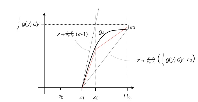
We want to approximate the function $g_{\#}$ by a piece-wise linear function, the red function in Figure 2, which is the mean of the indicated upper and lower bounds. To make that explicit note that in both cases $g=\widetilde{f}$ and $g={\rm id}\cdot\widetilde{f}$ we have $g(1)=-\eta\leq\sigma-1$. Now, the total hight of the building $H_{\rm tot}$ should be regarded as close to $\infty$ in the following sense: Let $\varepsilon_{0}:=\int_{0}^{\frac{\Delta z_{1}}{\Delta H_{\rm tot}}}g(y)\,dy$. In our main application in the next subsection we will have $z_{0}=46{\,\textrm{m}},z_{1}=110{\,\textrm{m}}$ and $H_{\rm tot}=438{\,\textrm{m}}$, so $\frac{\Delta z_{1}}{\Delta H_{\rm tot}}<0.164$, and because $g$ is convex we find

We estimate the function $g_{\#}$ from above by

and from below by

The maximal difference between $g_{+}$ and $g_{-}$ is at the gluing point $z_{2}$ (Figure 2). We have $z_{2}=z_{1}+\frac{z_{1}-z_{0}}{\sigma-1}\int_{0}^{1}g(y)\,dy$. The red function $g_{\rm red}:=\frac{1}{2}(g_{+}+g_{-})$ is the mean of $g_{+}$ and $g_{-}$. Therefore the maximal possible error between $g_{\#}$ and $g_{\rm red}$ is smaller than

at the point $z_{2}$. Here $q=\int_{0}^{1}g(y)\,dy$ which is either $q=q_{0}(f)$ or $q=q_{1}(f)$.

To derive the modified Crush-Down Equation $\frac{d}{dt}p(t)=m_{0}g+\Delta m(z(t))g-F(z(t))$ we just need compute the aggregated momentum $p(t)$ of the top section and the middle section. We have

References

- [BaLe11] Bažant, Z. P.; Le, J.-L.: Why the Observed Motion History of World Trade Center Towers Is Smooth, Journal of Engineering Mechanics, Vol. 137, No. 1, (2011), http://www.civil.northwestern.edu/people/bazant/PDFs/Papers/499.pdf
- [BaLe16] Bažant, Z. P.; Le, J.-L.: Mechanics of Collapse of WTC Towers Clarified by Recent Column Buckling Tests of Korol and Sivakumaran, Northwestern University, Report SEGIM No. 16-08c (2016), http://www.civil.northwestern.edu/people/bazant/PDFs/Papers/00-WTC-2016-buckling.pdf
- [BaVe07] Bažant, Z. P.; Verdure, M.: Mechanics of Progressive Collapse: Learning from World Trade Center and Building Demolitions, Journal of Engineering Mechanics, Vol. 133, No. 3, (2007), http://www.civil.northwestern.edu/people/bazant/PDFs/Papers/466.pdf
- [BaZh02] Bažant, Z. P.; Zhou, Y.: Why Did the World Trade Center Collapse?—Simple Analysis, Journal of Engineering Mechanics, Vol. 128, No. 1, (2002), http://www.civil.northwestern.edu/people/bazant/PDFs/Papers/405.pdf
- [BLGB08] Bažant, Z. P; Le, J.-L.; Greening F. R.; Benson D. B.: What Did and Did Not Cause Collapse of World Trade Center Twin Towers in New York? Journal of Engineering Mechanics, Vol. 134, No. 10, (2008),, http://www.civil.northwestern.edu/people/bazant/PDFs/Papers/476.pdf
- [NIST] National Institute of Standards and Technology: NCSTAR 1: Federal Building and Fire Safety Investigation of the World Trade Center Disaster: Final Report of the National Construction Safety Team on the Collapses of the World Trade Center Tower, (2005), https://ws680.nist.gov/publication/get_pdf.cfm?pub_id=909017
- [Schn17a] Schneider, A.: Energy Estimates of Progressive Floor Collapses, (2017), preprint available at http://front.math.ucdavis.edu/search?a=ansgar+schneider
- [Schn17b] Schneider, A.: The Late Jolt – Re-Examining the World Trade Center Catastrophe, (2017), preprint available at http://front.math.ucdavis.edu/search?a=ansgar+schneider
- [SSJ13] Szulandziński, G.; Szamboti, A.; Johns, R.: Some Misunderstandings Related to WTC Collapse Analysis, International Journal of Protective Structures, Volume 4, Number 2, (2013), , http://911speakout.org/wp-content/uploads/Some-Misunderstandings-Related-to-WTC-Collapse-Analysis.pdf
- [Uric07] Urich, G. H.:Analysis of the Mass and Potential Energy of World Trade Center Tower 1 , Journal of 9/11 Studies, (2007), http://www.journalof911studies.com/letters/wtc_mass_and_energy.pdf