A Distributed Particle-PHD Filter with Arithmetic-Average PHD Fusion

Tiancheng Li Franz Hlawatsch ^†^†thanks: T. Li is with the School of Automation, Northwestern Polytechnical University, Xi’an 710129, China and also with the BISITE group, University of Salamanca, 37007 Salamanca, Spain; e-mail: t.c.li@usal.es, t.c.li@mail.nwpu. edu.cn.^†^†thanks: F. Hlawatsch is with the Institute of Telecommunications, TU Wien, Vienna, Austria and also with Brno University of Technology, Brno, Czech Republic; e-mail: franz.hlawatsch@tuwien.ac.at.^†^†thanks: This work was partially supported by the Marie Skłodowska-Curie Individual Fellowship (H2020-MSCA-IF-2015) under Grant 709267 and by the Austrian Science Fund (FWF) under Grant P27370-N30.

Abstract

We propose a particle-based distributed PHD filter for tracking an unknown, time-varying number of targets. To reduce communication, the local PHD filters at neighboring sensorscommunicate Gaussian mixture (GM) parameters. In contrast to most existing distributed PHD filters, our filter employs an “arithmetic average” fusion. For particles–GM conversion, we use a method that avoids particle clustering and enables a significance-based pruning of the GM components. For GM–particles conversion, we develop an importance sampling based method that enables a parallelization of filtering and dissemination/fusion operations. The proposed distributed particle-PHD filter is able to integrate GM-based local PHD filters. Simulations demonstrate the excellent performance and small communication and computation requirements of our filter.

Index Terms:

Distributed multitarget tracking, distributed PHD filter, average consensus, flooding, probability hypothesis density, random finite set, Gaussian mixture, sequential Monte Carlo, importance sampling, arithmetic average fusion.

I Introduction

The probability hypothesis density (PHD) filter is a popular method for tracking an unknown, time-varying number of targets in the presence of clutter and missed detections [1, 2, 3]. In decentralized sensor networks, a distributed extension of the PHD filter can be employed where each sensor runs a local PHD filter and exchanges relevant information with neighboring sensors. For the local PHD filters, a Gaussian mixture (GM) implementation [4, 5, 6, 7, 8, 9, 10] or a particle-based implementation [11, 12, 13, 14] is typically used. For distributed data fusion, most existing distributed PHD filters perform a “geometric average” (GA) fusion of the local posterior PHDs [11, 12, 4, 5, 6, 7]; this type of fusion is also known as (generalized) covariance intersection [15, 16, 17, 18, 19, 20]. However, GA fusion of PHDs has been observed to suffer from certain deficiencies: it performs poorly in the case of closely spaced targets [9, 10]; it incurs a delay in detecting new targets [6, 10]; it is sensitive to missing measurements [8, 7]; and it does not lead to consistent fusion of cardinality distributions and thus tends to underestimate the number of targets [21].

In this paper, we propose a distributed PHD filter method that performs an “arithmetic average” (AA) fusion of the localposterior PHDs. AA fusion of PHDs first appeared indirectly in the context of centralized multisensor PHD filtering, as an implicit consequence of AA fusion of the generalized likelihood functions of multiple sensors [22]. It was used explicitly and in the context of distributed PHD filtering in [8, 10] (based on a GM implementation of the local PHD filters) and in [13, 14] (based on a particle implementation of the local PHD filters and a straightforward particle-based dissemination/fusion scheme). AA fusion of PHDs was demonstrated in [10, 13, 14] to outperform GA fusion of PHDs in the sense of better filtering accuracy, higher reliability in scenarios with strong clutter and/or frequent missed detections, and lower computational complexity.

The proposed distributed PHD filter employs a particle implementation of the local PHD filters for the sake of maximum suitability for nonlinear and/or non-Gaussian system models. Straightforward fusion of particle representations of the local and fused PHDs imposes high communication requirements [13, 14]. By contrast, our filter has low communication requirements because GM parameters are communicated. This also allows our particle-based local PHD filters to be easily combined with GM-based local PHD filters within a heterogeneous network architecture.

For converting particle representations into GM representations, we propose a data-driven method that avoids a clustering of the particles. This method generates from the particle representation one Gaussian component for each measurement that has a significant impact on the particle weights. The overall approach is inspired by a scheme for estimate extraction proposed in [23, 24, 25]. For converting the GMs produced by AA fusion into particle representations, we propose a method that is based on importance sampling (IS) [26, Ch. 3.3]. This method does not require sampling from the fused GM, thereby enabling a parallelization of filtering and dissemination/fusion operations. This allows more dissemination/fusion iterations to be performed compared to protocols where the filtering and dissemination/fusion operations must be performed serially. Overall, the main contribution of this paper is to devise an AA fusion-based distributed particle-PHD filter that has low communication requirements and allows for a parallelization of filtering and dissemination/fusion operations.

The paper is organized as follows. The system model is described in Section II. Section III discusses the basic operation of the particle-based local PHD filters and presents a measurement-based weight decomposition. Section IV provides a motivation and outline of the proposed distributed PHD filter. Section V describes a method for converting particle representations into GM representations. Section VI discusses two schemes for GM dissemination and fusion. An IS method for converting the fused GM into a particle representation is proposed in Section VII. Section VIII presents two further stages of the proposed distributed PHD filter. Section IX provides a summary of the overall method, discusses the parallelization of filtering and fusion, and analyzes the communication cost. Simulation results are reported in Section X.

II System Model

We consider $N_{k}$ targets with random states $\mathbf{x}_{k}^{(\nu)}\!\!\in\!\mathbb{R}^{d}\hskip-0.85358pt$ , $\nu=1,2,\ldots,N_{k}$ at discrete time $k$ . The number of targets, $N_{k}$ , is unknown, time-varying, and considered random. Accordingly, the collection of target states is modeled by a random finite set (RFS) $X_{k}=\big\{\mathbf{x}_{k}^{(1)},\mathbf{x}_{k}^{(2)},\ldots,\mathbf{x}_{k}^{(N_{k})}\big\}$ with random cardinality $N_{k}\!=\hskip-0.85358pt|X_{k}|$ [27]. The cardinality distribution $\rho(n)\triangleq\mathrm{Pr}[N_{k}\!=\!n]$ is the probability mass function of $N_{k}$ . A target with state $\mathbf{x}_{k-1}$ at time $k\!-\!1$ continues to exist at time $k$ with probability $p_{k}^{\text{S}}(\mathbf{x}_{k-1})$ (“survival probability”) or disappears with probability $1\!-\hskip-0.85358ptp_{k}^{\text{S}}(\mathbf{x}_{k-1})$ . In the former case, its new state $\mathbf{x}_{k}\!\in\!X_{k}$ is distributed according to a transition probability density function (pdf) $f_{k}(\mathbf{x}_{k}|\mathbf{x}_{k-1})$ . There may also be newborn targets, whose states are modeled by a Poisson RFS with intensity function $\gamma_{k}(\mathbf{x}_{k})$ [28].

There are $S$ sensors indexed by $s\hskip-0.85358pt\in\hskip-0.85358pt\{1,2,\ldots,S\}$ . At time $k$ , each sensor $s$ observes an RFS of measurements $Z_{s,k}\hskip-0.85358pt=$ $\big\{{\mathbf{z}_{s,k}^{(1)},\ldots,\mathbf{z}_{s,k}^{(M_{s,k})}}\big\}$ , where $M_{s,k}$ is the number of measurements observed by sensor $s$ at time $k$ . We denote by ${\cal S}_{s}\hskip-0.85358pt\subseteq$ $\{1,2,\ldots,S\}\hskip-0.85358pt\setminus\hskip-0.85358pt\{s\}$ the set of sensors that are connected to sensor $s$ by a communication link, and we refer to these sensors as the neighbors of sensor $s$ . We assume that the sensor network is connected, i.e., each sensor can be reached from each other sensor by one or multiple communication hops. A target with state $\mathbf{x}_{k}$ is “detected” by sensor $s$ with probability $p_{s,k}^{\text{D}}(\mathbf{x}_{k})$ (“detection probability”) or “missed” by sensor $s$ with probability $1\!-\hskip-0.85358ptp_{s,k}^{\text{D}}(\mathbf{x}_{k})$ . In the former case, the target generates a measurement $\mathbf{z}_{k}\!\in\!Z_{k}$ , which is distributed according to the pdf $g_{s,k}(\mathbf{z}_{k}\big|\mathbf{x}_{k})$ . There may also be clutter measurements, which are modeled by a Poisson RFS with intensity function (PHD) $\kappa_{s,k}(\mathbf{z}_{k})$ . The multitarget state evolution and measurement processes are assumed to satisfy the independence assumptions discussed in [1].

III Local Particle-PHD Filters

Each sensor runs a local PHD filter that uses the local measurement set $Z_{s,k}$ and communicates with its neighbors $r\!\in\!{\cal S}_{s}$ to exchange relevant information. Let us, at first, consider the local PHD filter without any cooperation.

III-A Propagation of the Local Posterior PHD

The local PHD filter propagates the local posterior PHD over time $k$ . Let $Z_{s,1:k}=(Z_{s,1},\ldots,Z_{s,k})$ comprise the local measurements $Z_{s,k^{\prime}}$ observed by sensor $s$ up to time $k$ . Furthermore, for a region $\mathcal{R}\!\subseteq\!\mathbb{R}^{d}$ , let $N_{k}^{\mathcal{R}}\triangleq\hskip 0.85358pt|X_{k}\!\cap\hskip-0.85358pt\mathcal{R}|$ denote the number of those targets whose states are in $\mathcal{R}$ . Then, the local posterior PHD at sensor $s$ , $D_{s,k}(\mathbf{x}|Z_{s,1:k})$ , is defined as the function of $\mathbf{x}\!\in\!\mathbb{R}^{d}$ whose integral over a region $\mathcal{R}\!\subseteq\!\mathbb{R}^{d}$ equals the posterior expectation of $N_{k}^{\mathcal{R}}$ , i.e. [27]

\int_{\mathcal{R}}\!\hskip-0.85358ptD_{s,k}(\mathbf{x}|Z_{s,1:k})\hskip 0.85358pt\mathrm{d}\mathbf{x}=\mathrm{E}\big[N_{k}^{\mathcal{R}}\big|Z_{s,1:k}\big]\hskip 0.85358pt.

(1)

In particular, for $\mathcal{R}\!=\!\mathbb{R}^{d}$ , we have $N_{k}^{\mathbb{R}^{d}}\!=|X_{k}\cap\mathbb{R}^{d}|=|X_{k}|=N_{k}$ , and thus (1) becomes

\displaystyle\int_{\mathbb{R}^{d}}\!\hskip-0.85358ptD_{s,k}(\mathbf{x}|Z_{s,1:k})\hskip 0.85358pt\mathrm{d}\mathbf{x}=\mathrm{E}[N_{k}|Z_{s,1:k}]=\sum_{n=0}^{\infty}\!n\,\rho(n|Z_{s,1:k})\hskip 0.85358pt,

where $\rho(n|Z_{s,1:k})=\mathrm{Pr}[N_{k}\!=\!n|Z_{s,1:k}]$ . The posterior expectation of $N_{k}$ , $\mathrm{E}[N_{k}|Z_{s,1:k}]$ , is equal to the minimum mean square error (MMSE) estimate of $N_{k}$ from $Z_{s,1:k}$ [29], denoted $\hat{N}_{s,k}^{\text{MMSE}}\hskip-0.85358pt$ . Thus, Eq. () implies

\hat{N}_{s,k}^{\text{MMSE}}=\mathrm{E}[N_{k}|Z_{s,1:k}]=\hskip-0.85358pt\int_{\mathbb{R}^{d}}\!\hskip-0.85358ptD_{s,k}(\mathbf{x}|Z_{s,1:k})\hskip 0.85358pt\mathrm{d}\mathbf{x}\hskip 0.85358pt.

(3)

This is also known as the expected a posteriori (EAP) estimate of $N_{k}$ [1, 27].

The local PHD filter performs a time-recursive calculation of an approximation $\hat{D}_{s,k}(\mathbf{x}|Z_{s,1:k})$ of the local posterior PHD $D_{s,k}(\mathbf{x}|Z_{s,1:k})$ . In a prediction step, it converts the preceding approximate local posterior PHD $\hat{D}_{s,k-1}(\mathbf{x}|Z_{s,1:k-1})$ into a “predicted” PHD, denoted $D_{s,k|k-1}(\mathbf{x}|Z_{s,1:k-1})$ , via an expression involving $f_{k}(\mathbf{x}_{k}|\mathbf{x}_{k-1})$ , $p_{k}^{\text{S}}(\mathbf{x})$ , and $\gamma_{k}(\mathbf{x})$ [1]. In a subsequent update step, it converts $D_{s,k|k-1}(\mathbf{x}|Z_{s,1:k-1})$ into the approximate local posterior PHD $\hat{D}_{s,k}(\mathbf{x}|Z_{s,1:k})$ via anexpression involving $g_{s,k}(\mathbf{z}\big|\mathbf{x})$ , $p_{s,k}^{\text{D}}(\mathbf{x})$ , and $\kappa_{s,k}(\mathbf{z})$ [1, 2].

III-B Particle-Based Implementation

We use the particle-based implementation of the prediction and update steps proposed in [2]. The approximate local posterior PHD $\hat{D}_{s,k}(\mathbf{x}|Z_{s,1:k})$ is represented by the weighted particle set $\xi_{s,k}\hskip-0.85358pt\triangleq\hskip-0.85358pt\big\{\big(\mathbf{x}_{s,k}^{(j)}\hskip 0.85358pt,w_{s,k}^{(j)}\big)\big\}_{j=1}^{J_{s,k}}$ , which consists of $J_{s,k}$ particles $\mathbf{x}_{s,k}^{(j)}\!\in\!\mathbb{R}^{d}$ and weights $w_{s,k}^{(j)}\!\geq\!0$ , $j=1,2,\ldots,J_{s,k}$ . The sum of the

weights,

W_{s,k}\triangleq\sum_{j=1}^{J_{s,k}}w_{s,k}^{(j)}\hskip 0.85358pt,

(4)

approximates $\int_{\mathbb{R}^{d}}\hskip-0.85358pt\hat{D}_{s,k}(\mathbf{x}|Z_{s,1:k})\hskip 0.85358pt\mathrm{d}\mathbf{x}$ and, hence, $\int_{\mathbb{R}^{d}}\hskip-0.85358ptD_{s,k}(\mathbf{x}|Z_{s,1:k})\hskip 0.85358pt\mathrm{d}\mathbf{x}$ . Thus, it further follows with (3) that

W_{s,k}\approx\hat{N}_{s,k}^{\text{MMSE}}.

(5)

Propagating the approximate local posterior PHD (i.e., $\hat{D}_{s,k-1}(\mathbf{x}|Z_{s,1:k-1})\!\to\!\hat{D}_{s,k}(\mathbf{x}|Z_{s,1:k})$ ) is now approximated by propagating the weighted particle set, i.e., $\xi_{s,k-1}\!\to\!\xi_{s,k}$ . The time-recursive calculation of $\xi_{s,k}$ is done as follows [2]. For each previous particle $\mathbf{x}_{s,k-1}^{(j)}$ , $j\hskip-0.85358pt\in\hskip-0.85358pt\{1,\ldots,J_{s,k-1}\}$ , a current particle $\mathbf{x}_{s,k}^{(j)}$ is drawn from a proposal pdf $q_{s,k}\big(\mathbf{x};\mathbf{x}_{s,k-1}^{(j)},Z_{s,k}\big)$ . In addition, $L_{s,k}\hskip-0.85358pt\triangleq\hskip-0.85358ptJ_{s,k}\hskip-0.85358pt-\hskip-0.85358ptJ_{s,k-1}$ “newborn” particles $\mathbf{x}_{s,k}^{(j)}$ , $j\hskip-0.85358pt=\hskip-0.85358ptJ_{s,k-1}+1,\ldots,J_{s,k}$ are drawn from a proposal pdf $p_{s,k}(\mathbf{x};Z_{s,k})$ . Then, for each particle $\mathbf{x}_{s,k}^{(j)}$ , $j\hskip-0.85358pt\in\{1,\ldots,J_{s,k}\}$ , a “predicted” weight $w_{s,k|k-1}^{(j)}$ is calculated as

\displaystyle w_{s,k|k-1}^{(j)}\!=\hskip-0.85358pt\begin{cases}\displaystyle\frac{f_{k}\big(\mathbf{x}_{s,k}^{(j)}\big|\mathbf{x}_{s,k-1}^{(j)}\big)\hskip 0.85358ptw_{s,k-1}^{(j)}}{q_{s,k}\big(\mathbf{x}_{s,k}^{(j)};\mathbf{x}_{s,k-1}^{(j)},Z_{s,k}\big)}\hskip 0.85358pt,&\!\!\!j\hskip-0.85358pt=\hskip-0.85358pt1,\ldots,J_{s,k-1},\\[15.649pt] \displaystyle\frac{\gamma_{k}\big(\mathbf{x}_{s,k}^{(j)}\big)}{L_{s,k}\,p_{s,k}\big(\mathbf{x}_{s,k}^{(j)};Z_{s,k}\big)}\hskip 0.85358pt,&\!\!\!j\hskip-0.85358pt=\hskip-0.85358ptJ_{s,k-1}\!+\!\hskip-0.85358pt1,\ldots,J_{s,k}\hskip 0.85358pt.\end{cases}

Note that $J_{s,k}\hskip-0.85358pt=\hskip-0.85358ptJ_{s,k-1}+L_{s,k}$ . A simple choice of the first proposal pdf is $q_{s,k}\big(\mathbf{x};\mathbf{x}_{s,k-1}^{(j)},Z_{s,k}\big)=f_{k}\big(\mathbf{x}\big|\mathbf{x}_{s,k-1}^{(j)}\big)$ , in which case $w_{s,k|k-1}^{(j)}\!=\hskip-0.85358ptw_{s,k-1}^{(j)}$ for $j\hskip-0.85358pt=\hskip-0.85358pt1,\ldots,J_{s,k-1}$ .

For the calculation of the current weights $w_{s,k}^{(j)}$ , $j\hskip-0.85358pt=\hskip-0.85358pt1,\ldots,$ $J_{s,k}$ , we formally introduce a “pseudo-measurement” $\mathbf{z}_{0}$ representing the case of a missed detection at sensor $s$ , and, accordingly, we consider an extended measurement set $Z_{s,k}^{0}\!\triangleq$ $\{\mathbf{z}_{0}\}\hskip 0.42677pt\cup\hskip 0.28453ptZ_{s,k}\!=\!\big\{\mathbf{z}_{0},{\mathbf{z}_{s,k}^{(1)},\ldots,\mathbf{z}_{s,k}^{(M_{s,k})}}\big\}$ . Then, the weight expression in [2, Eq. (22)] can be formulated as the

sum [23, 24, 25]

w_{s,k}^{(j)}=\!\sum_{\mathbf{z}\in Z_{s,k}^{0}}\!\hskip-0.85358pt\omega_{s,k}^{(j)}(\mathbf{z})\hskip 0.85358pt,\quad j\hskip-0.85358pt=\hskip-0.85358pt1,\ldots,J_{s,k}\hskip 0.85358pt,\vskip-7.11317pt

(7)

where

\hskip 2.84526pt\omega_{s,k}^{(j)}(\mathbf{z})=\begin{cases}\big(1\!-\hskip-0.85358ptp_{s,k}^{\text{D}}\big(\mathbf{x}_{s,k}^{(j)}\big)\big)\hskip 0.85358ptw_{s,k|k-1}^{(j)}\hskip 0.85358pt,&\!\mathbf{z}\hskip-0.85358pt=\hskip-0.85358pt\mathbf{z}_{0}\\[7.11317pt] \displaystyle\frac{p_{s,k}^{\text{D}}\big(\mathbf{x}_{s,k}^{(j)}\big)\hskip 0.85358ptg_{s,k}\big(\mathbf{z}\big|\mathbf{x}_{s,k}^{(j)}\big)\hskip 0.85358ptw_{s,k|k-1}^{(j)}}{\kappa_{s,k}(\mathbf{z})+G_{s,k}(\mathbf{z})}\hskip 0.85358pt,&\!\mathbf{z}\hskip-0.85358pt\in\!Z_{s,k}\hskip 0.85358pt,\end{cases}\hskip-14.22636pt

(8)

with $G_{s,k}(\mathbf{z})\triangleq\sum_{j=1}^{J_{s,k}}p_{s,k}^{\text{D}}\big(\mathbf{x}_{s,k}^{(j)}\big)\hskip 0.85358ptg_{s,k}\big(\mathbf{z}\big|\mathbf{x}_{s,k}^{(j)}\big)\hskip 0.85358ptw_{s,k|k-1}^{(j)}$ . Expression (7) provides an expansion of $w_{s,k}^{(j)}$ into $|Z_{s,k}^{0}|\hskip-0.85358pt=M_{s,k}+1$ components $\omega_{s,k}^{(j)}(\mathbf{z})$ , each of which corresponds to one of the measurements $\mathbf{z}\!\in\!Z_{s,k}^{0}$ . We also introduce

\Omega_{s,k}(\mathbf{z})\hskip 0.85358pt\triangleq\hskip 0.85358pt\sum_{j=1}^{J_{s,k}}\omega_{s,k}^{(j)}(\mathbf{z})\hskip 0.85358pt,\quad\mathbf{z}\hskip-0.85358pt\in\!Z_{s,k}^{0}\hskip 0.85358pt.\vskip-1.42262pt

(9)

For $\mathbf{z}\hskip-0.85358pt\in\!Z_{s,k}$ , $\Omega_{s,k}(\mathbf{z})\hskip-0.85358pt=\hskip-0.85358ptG_{s,k}(\mathbf{z})/\big(\kappa_{s,k}(\mathbf{z})+G_{s,k}(\mathbf{z})\big)\hskip-0.85358pt\in\hskip-0.85358pt[0,1]$ , which provides an estimate of the probability that measurement $\mathbf{z}$ originates from a target. For $\mathbf{z}\hskip-0.85358pt=\hskip-0.85358pt\mathbf{z}_{0}$ , $\Omega_{s,k}(\mathbf{z}_{0})\hskip-0.85358pt=\sum_{j=1}^{J_{s,k}}\big(1\!-\hskip-0.85358ptp_{s,k}^{\text{D}}\big(\mathbf{x}_{s,k}^{(j)}\big)\big)\hskip 0.85358ptw_{s,k|k-1}^{(j)}$ provides an estimate of the number of missed detections. Note that

\sum_{\mathbf{z}\in Z_{s,k}^{0}}\!\!\Omega_{s,k}(\mathbf{z})=\sum_{j=1}^{J_{s,k}}\sum_{\mathbf{z}\in Z_{s,k}^{0}}\!\!\omega_{s,k}^{(j)}(\mathbf{z})=\sum_{j=1}^{J_{s,k}}w_{s,k}^{(j)}=W_{s,k}\hskip 0.85358pt,

(10)

where (7) and (4) were used.

IV Motivation and Outline of the ProposedPHD Fusion Scheme

The proposed distributed PHD filter uses information fused among the sensors to “re-weight” the particles of the local PHD filters such that the resulting new PHD approximates the AA of the local PHDs. Forming the AA can be motivated as follows. Suppose sensor $s$ wishes to estimate the number of targets in a region $\mathcal{R}\!\subseteq\!\mathbb{R}^{d}$ , $N_{k}^{\mathcal{R}}\hskip-0.85358pt=\hskip-0.85358pt|X_{k}\cap\mathcal{R}|$ , via the estimator (cf. (1)) $\hat{N}_{s,k}^{\mathcal{R},\text{loc}}\hskip-0.85358pt=\hskip-0.85358pt\int_{\mathcal{R}}\hskip-0.85358pt\hat{D}_{s,k}(\mathbf{x}|Z_{s,1:k})\hskip 0.85358pt\mathrm{d}\mathbf{x}$ . Since $Z_{s,1:k}$ is affected by clutter and missed detections, $\hat{N}_{s,k}^{\mathcal{R},\text{loc}}$ may be quite different from $N_{k}^{\mathcal{R}}$ . For example, if one target is in $\mathcal{R}$ , i.e., $N_{k}^{\mathcal{R}}\!=\!1$ , sensor $s$ may fail to detect that target, resulting in $\hat{N}_{s,k}^{\mathcal{R},\text{loc}}\!\hskip-0.85358pt\approx\hskip-0.85358pt0$ ; or if no target is in $\mathcal{R}$ , i.e., $N_{k}^{\mathcal{R}}\!=\hskip-0.85358pt0$ , a false alarm (clutter) at sensor $s$ may lead to $\hat{N}_{s,k}^{\mathcal{R},\text{loc}}\!\hskip-0.85358pt\approx\!1$ . On the other hand, because the clutter and the missed detections at different sensors $s\!\in\!\cal{S}$ are not identical—in fact, they are assumed independent across the sensors—one can expect that the AA of the $\hat{N}_{s,k}^{\mathcal{R},\text{loc}}\hskip-0.85358pt$ , $\hat{N}_{1:S,k}^{\mathcal{R}}\hskip-0.85358pt\triangleq\sum_{s=1}^{S}\hskip-0.85358pt\hat{N}_{s,k}^{\mathcal{R},\text{loc}}/S$ , is a more robust estimate of $N_{k}^{\mathcal{R}}$ . This AA can be expressed

\hat{N}_{1:S,k}^{\mathcal{R}}=\frac{1}{S}\sum_{s=1}^{S}\int_{\mathcal{R}}\!\!\hat{D}_{s,k}(\mathbf{x}|Z_{s,1:k})\hskip 0.85358pt\mathrm{d}\mathbf{x}=\hskip-0.85358pt\int_{\mathcal{R}}\!\!\hat{D}_{k}(\mathbf{x}|Z_{1:S,1:k})\hskip 0.85358pt\mathrm{d}\mathbf{x}\hskip 0.85358pt,\vskip 1.42262pt

with the AA of the local PHDs

\hat{D}_{k}(\mathbf{x}|Z_{1:S,1:k})\triangleq\frac{1}{S}\sum_{s=1}^{S}\hat{D}_{s,k}(\mathbf{x}|Z_{s,1:k})\hskip 0.85358pt.\vskip-1.42262pt

(11)

Thus, $\hat{N}_{1:S,k}^{\mathcal{R}}$ is obtained by integrating the AA of the local PHDs over $\mathcal{R}$ . This motivates a fusion of the local PHDs $\hat{D}_{s,k}(\mathbf{x}|Z_{s,1:k})$ —thereby combining all the local measurements $Z_{s,1:k}$ , $s=1,\ldots,S$ —by calculating the AA of the $\hat{D}_{s,k}(\mathbf{x}|Z_{s,1:k})$ : we can expect that this compensates the effects of clutter and missed detections to some extent. In addition, the AA fusion of the local PHDs can be motivated theoretically by the fact that the fused PHD minimizes the sum of the Cauchy-Schwarz divergences relative to the local PHDs [30, 13].

To reduce the amount of intersensor communication, the information exchanged between neighboring sensors in our approach consists of GM parameters rather than particles and weights. This necessitates conversions between particle and GM representations. The proposed AA-based fusion scheme thus consists of the following

steps:

1.

Each sensor $s$ converts its weighted particle set $\xi_{s,k}=\big\{\big(\mathbf{x}_{s,k}^{(j)}\hskip 0.85358pt,w_{s,k}^{(j)}\big)\big\}_{j=1}^{J_{s,k}}$ into a GM (see Section V) and broadcasts the GM parameters to the neighboring sensors $r\!\in\!{\cal S}_{s}$ .
2.

Each sensor $s$ broadcasts its local cardinality estimate $W_{s,k}$ (see (4), (5)) to the neighboring sensors $r\!\in\!{\cal S}_{s}$ .
3.

The GM parameters of each sensor $s$ are fused with those received from the other sensors via a distributed dissemination/fusion scheme; see Section VI.
4.

The local cardinality estimate $W_{s,k}$ of each sensor $s$ is fused with those received from the other sensors via a distributed dissemination/fusion scheme; see Section VIII-A [31].
5.

At each sensor $s$ , the local particle weights $w_{s,k}^{(j)}$ are modified based on the fused GM parameters and the fused cardinality estimate; see Sections VII and VIII-A.

V Particles–GM Conversion

In Step 1, the local weighted particle set $\xi_{s,k}=\big\{\big(\mathbf{x}_{s,k}^{(j)}\hskip 0.85358pt,$ $w_{s,k}^{(j)}\big)\big\}_{j=1}^{J_{s,k}}$ is converted into a GM representation. Our conversion method differs from previous methods [32, 33, 34, 35, 12, 36, 37]in that it is based on the weight expansion in (7), i.e., $w_{s,k}^{(j)}=$ $\sum_{\mathbf{z}\in Z_{s,k}^{0}}\hskip-0.85358pt\omega_{s,k}^{(j)}(\mathbf{z})$ . In our method, each of the $|Z_{s,k}^{0}|\hskip-0.85358pt=\hskip-0.85358ptM_{s,k}\hskip-0.85358pt+\hskip-0.85358pt1$ extended measurements $\mathbf{z}\hskip-0.85358pt\in\hskip-0.85358ptZ_{s,k}^{0}\!=\hskip-0.85358pt\big\{\mathbf{z}_{0},\mathbf{z}_{s,k}^{(1)},\ldots,\mathbf{z}_{s,k}^{(M_{s,k})}\big\}$ potentially corresponds to one Gaussian component (GC) $\mathcal{N}\big(\mathbf{x};\bm{\mu}_{s,k}(\mathbf{z}),\bm{\Sigma}_{s,k}(\mathbf{z})\big)$ . Here, $\mathcal{N}(\mathbf{x};\bm{\mu},\bm{\Sigma})$ denotes a Gaussian pdf with mean vector $\bm{\mu}$ and covariance matrix $\bm{\Sigma}$ . The GC $\mathcal{N}\big(\mathbf{x};\bm{\mu}_{s,k}(\mathbf{z}),\bm{\Sigma}_{s,k}(\mathbf{z})\big)$ is meant to represent the weighted particle set $\big\{\big(\mathbf{x}_{s,k}^{(j)}\hskip 0.85358pt,\omega_{s,k}^{(j)}(\mathbf{z})\big)\big\}_{j=1}^{J_{s,k}}$ . The mean vector $\bm{\mu}_{s,k}(\mathbf{z})$ and covariance matrix $\bm{\Sigma}_{s,k}(\mathbf{z})$ are derived from the respective weight components $\omega_{s,k}^{(j)}(\mathbf{z})$ and the particles $\mathbf{x}_{s,k}^{(j)}$

	$\displaystyle\bm{\mu}_{s,k}(\mathbf{z})$	$\displaystyle=\sum_{j=1}^{J_{s,k}}\bar{\omega}_{s,k}^{(j)}(\mathbf{z})\,\mathbf{x}_{s,k}^{(j)},$		(12)
	$\displaystyle\bm{\Sigma}_{s,k}(\mathbf{z})$	$\displaystyle=\sum_{j=1}^{J_{s,k}}\bar{\omega}_{s,k}^{(j)}(\mathbf{z})\hskip 0.85358pt\big(\mathbf{x}_{s,k}^{(j)}\hskip-0.85358pt-\hskip-0.85358pt\bm{\mu}_{s,k}(\mathbf{z})\big)\hskip 0.85358pt\big(\mathbf{x}_{s,k}^{(j)}\hskip-0.85358pt-\hskip-0.85358pt\bm{\mu}_{s,k}(\mathbf{z})\big)^{\hskip-0.85358pt\text{T}},$

where $\bar{\omega}_{s,k}^{(j)}(\mathbf{z})=\omega_{s,k}^{(j)}(\mathbf{z})/\sum_{j^{\prime}=1}^{J_{s,k}}\omega_{s,k}^{(j^{\prime})}(\mathbf{z})=\omega_{s,k}^{(j)}(\mathbf{z})/\Omega_{s,k}(\mathbf{z})$ with $\omega_{s,k}^{(j)}(\mathbf{z})$ given by (8). In the overall GM-based PHD (briefly referred to as GM-PHD), the GC $\mathcal{N}\big(\mathbf{x};\bm{\mu}_{s,k}(\mathbf{z}),$ $\bm{\Sigma}_{s,k}(\mathbf{z})\big)$ is multiplied by the weight $\Omega_{s,k}(\mathbf{z})=\sum_{j=1}^{J_{s,k}}\omega_{s,k}^{(j)}(\mathbf{z})$ (see (9)). Thus, there is one weighted GC $\Omega_{s,k}(\mathbf{z})\,\mathcal{N}\big(\mathbf{x};$ $\bm{\mu}_{s,k}(\mathbf{z}),\bm{\Sigma}_{s,k}(\mathbf{z})\big)$ for each measurement $\mathbf{z}\hskip-0.85358pt\in\hskip-0.85358ptZ_{s,k}^{0}$ .

The overall GM-PHD is meant to represent the local weighted particle set $\xi_{s,k}=\big\{\big(\mathbf{x}_{s,k}^{(j)}\hskip 0.85358pt,w_{s,k}^{(j)}\big)\big\}_{j=1}^{J_{s,k}}$ . Because $w_{s,k}^{(j)}$ $=\sum_{\mathbf{z}\in Z_{s,k}^{0}}\hskip-0.85358pt\omega_{s,k}^{(j)}(\mathbf{z})$ , the overall GM-PHD is ideally taken to be the sum of all the weighted GCs, i.e.,

D_{s,k}^{\text{GM,full}}(\mathbf{x})\hskip 0.85358pt\triangleq\!\sum_{\mathbf{z}\in Z_{s,k}^{0}}\!\!\Omega_{s,k}(\mathbf{z})\,\mathcal{N}\big(\mathbf{x};\bm{\mu}_{s,k}(\mathbf{z}),\bm{\Sigma}_{s,k}(\mathbf{z})\big)\hskip 0.85358pt.\vskip-1.42262pt

(14)

This provides an approximate GM representation of $\hat{D}_{s,k}(\mathbf{x}|Z_{s,1:k})$ . However, to further reduce the communication cost, we restrict the sum (14) to the GCs corresponding to “significant” measurements. (We note that a similar restriction was used previously for estimate extraction in [23, 24, 25].) The subset of significant measurements, $Z_{s,k}^{\text{S}}\!\hskip-0.85358pt\subseteq\!Z_{s,k}^{0}$ , is defined as the set of those $\mathbf{z}\!\in\!Z_{s,k}^{0}$ for which $\Omega_{s,k}(\mathbf{z})$ in (9) is above a threshold $T_{\Omega}$ , where $0\!<\!T_{\Omega}\!<\!1$ . In other words, the GM at sensor $s$ contains a GC for $\mathbf{z}\hskip-0.85358pt\in\!Z_{s,k}$ if the estimated probability that the measurement $\mathbf{z}$ originates from a target (given by $\Omega_{s,k}(\mathbf{z})$ ) is above $T_{\Omega}$ , and it contains a GC for $\mathbf{z}_{0}$ if the estimated number of missed detections (given by $\Omega_{s,k}(\mathbf{z}_{0})$ ) is above $T_{\Omega}$ . Thus, the local GM-PHD is taken to be

D_{s,k}^{\text{GM}}(\mathbf{x})\hskip 0.85358pt\triangleq\!\sum_{\mathbf{z}\in Z_{s,k}^{\text{S}}}\!\!\Omega_{s,k}(\mathbf{z})\,\mathcal{N}\big(\mathbf{x};\bm{\mu}_{s,k}(\mathbf{z}),\bm{\Sigma}_{s,k}(\mathbf{z})\big)\hskip 0.85358pt.\vskip-1.42262pt

(15)

This can be interpreted as the GM-PHD corresponding to theparticle set $\big\{\big(\mathbf{x}_{s,k}^{(j)}\hskip 0.85358pt,\breve{w}_{s,k}^{(j)}\big)\big\}_{j=1}^{J_{s,k}}$ whose weights $\breve{w}_{s,k}^{(j)}$ are defined by summing the $\omega_{s,k}^{(j)}(\mathbf{z})$ only over the significant measurements, i.e., $\breve{w}_{s,k}^{(j)}\!=\!\sum_{\mathbf{z}\in Z_{s,k}^{\text{S}}}\!\omega_{s,k}^{(j)}(\mathbf{z})$ . We note that an alternative definition of a significant measurement subset $Z_{s,k}^{\text{S}}$ and, thus, of $D_{s,k}^{\text{GM}}(\mathbf{x})$ is to choose the $N_{\Omega}\hskip-0.85358pt\triangleq\hskip-0.85358pt\mathrm{round}\hskip 0.85358pt\{W_{s,k}\}$ GCs with the largest $\Omega_{s,k}(\mathbf{z})$ , $\mathbf{z}\!\in\!Z_{s,k}^{0}$ . Here, $W_{s,k}\!=\!\sum_{\mathbf{z}\in Z_{s,k}^{0}}\!\!\Omega_{s,k}(\mathbf{z})$ according to (10), and we recall from (5) that $W_{s,k}$ approximates the MMSE estimate $\hat{N}_{s,k}^{\text{MMSE}}\hskip-0.85358pt$ .

The suppression of GCs in (15) is motivated by the notion that “insignificant” measurements are likely to be false alarms (clutter). However, if an insignificant measurement is not a false alarm after all, we can expect that it is not suppressed at most of the other sensors, and thus the erroneous suppression at sensor $s$ will be compensated by the subsequent AA fusion. This is an advantage of AA fusion over GA fusion.

The GM parameter set underlying the local GM-PHD $D_{s,k}^{\text{GM}}(\mathbf{x})$ in (15) is

\mathcal{G}_{s,k}\triangleq\big\{\big(\Omega_{s,k}(\mathbf{z}),\bm{\mu}_{s,k}(\mathbf{z}),\bm{\Sigma}_{s,k}(\mathbf{z})\big)\big\}_{\mathbf{z}\in Z_{s,k}^{\text{S}}}.

(16)

All the further operations of our distributed PHD filter are based on $\mathcal{G}_{s,k}$ ; the GM-PHD $D_{s,k}^{\text{GM}}(\mathbf{x})$ itself is never calculated. These further operations comprise a distributed fusion of the local GM parameter sets and of the local cardinality estimates, the conversion of the fused GM representations into particle representations, a scaling of the particle weights, and the calculation of state estimates. A detailed presentation of these steps will be given in Sections VI–IX.

VI Two GM Dissemination/Fusion Schemes

Once the local GM parameter sets $\mathcal{G}_{s,k}$ are available at the respective sensors $s$ , they are disseminated and fused via a distributed scheme. The goal of this scheme is to obtain, at each sensor $s$ , a GM parameter set that approximately corresponds to the AA of all the local GM-PHDs,

\bar{D}_{k}^{\text{GM}}(\mathbf{x})\triangleq\frac{1}{S}\sum_{s=1}^{S}D_{s,k}^{\text{GM}}(\mathbf{x})\hskip 0.85358pt.

(17)

Note that this equals (11) except that $\hat{D}_{s,k}(\mathbf{x}|Z_{s,1:k})$ is replaced by $D_{s,k}^{\text{GM}}(\mathbf{x})$ . Next, we discuss two alternative schemes for disseminating and fusing the local GM parameter sets.

VI-A GM Flooding

In the flooding scheme [36], each sensor $s$ first broadcasts to its neighbors $r\!\in\!{\cal S}_{s}$ its GM parameter set $\mathcal{G}_{s,k}\hskip-0.85358pt=\big\{\big(\Omega_{s,k}(\mathbf{z}),$ $\bm{\mu}_{s,k}(\mathbf{z}),\bm{\Sigma}_{s,k}(\mathbf{z})\big)\big\}_{\mathbf{z}\in Z_{s,k}^{\text{S}}}$ and receives their GM parameter sets $\mathcal{G}_{r,k}\hskip-0.85358pt=\hskip-0.85358pt\big\{\big(\Omega_{r,k}(\mathbf{z}),\bm{\mu}_{r,k}(\mathbf{z}),\bm{\Sigma}_{r,k}(\mathbf{z})\big)\big\}_{\mathbf{z}\in Z_{r,k}^{\text{S}}}\hskip-0.85358pt$ , $r\!\in\!{\cal S}_{s}$ . Each sensor then augments its own GM parameter set $\mathcal{G}_{s,k}$ by the neighbor GM parameter sets $\mathcal{G}_{r,k}$ , $r\!\in\!{\cal S}_{s}$ , resulting in $\mathcal{G}_{s,k}^{\text{F}[1]}\hskip-0.85358pt=$ $\bigcup_{r\in\{s\}\cup{\cal S}_{s}}\hskip-0.85358pt\mathcal{G}_{r,k}$ . In the subsequent flooding iteration $i\hskip-0.85358pt\in\hskip-0.85358pt\{2,3,$ $\ldots\}$ , each sensor $s$ broadcasts to its neighbors the augmented set $\mathcal{G}_{s,k}^{\text{F}[i-1]}$ with the exception of the elements already broadcast (the sensor keeps track of all the elements it already broadcast [36]) and receives the new elements of the neighbors’ augmented sets $\mathcal{G}_{r,k}^{\text{F}[i-1]}\hskip-0.85358pt$ . This results in the new augmented set

\mathcal{G}_{s,k}^{\text{F}[i]}=\!\bigcup_{r\in\{s\}\cup{\cal S}_{s}}\!\!\!\mathcal{G}_{r,k}^{\text{F}[i-1]}\hskip 0.85358pt.\vskip-4.2679pt

(18)

This recursion is initialized with $\mathcal{G}_{s,k}^{\text{F}[0]}\!=\hskip-0.85358pt\mathcal{G}_{s,k}$ .

After the final flooding iteration $i\!=\!I$ (the choice of $I$ will be discussed in Section IX-A), the augmented parameter set at sensor $s$ is equal to

\mathcal{G}_{s,k}^{\text{F}[I]}=\hskip-0.85358pt\bigcup_{r\in{\cal S}_{s}^{[I]}}\!\!\mathcal{G}_{r,k}\hskip 0.85358pt,\vskip-4.2679pt

(19)

where ${\cal S}_{s}^{[I]}\!\subseteq\hskip-0.85358pt\{1,2,\ldots,S\}$ denotes the set of all those sensors that are at most $I$ hops away from sensor $s$ , including sensor $s$ itself. At this point, sensor $s$ would be able to calculate the AA of all the GM-PHDs whose GM parameters are contained in $\mathcal{G}_{s,k}^{[I]}$ ,

i.e.,

D_{s,k}^{\text{GM}[I]}(\mathbf{x})=\frac{1}{\big|{\cal S}_{s}^{[I]}\big|}\hskip-0.85358pt\sum_{r\in{\cal S}_{s}^{[I]}}\!\!D_{r,k}^{\text{GM}}(\mathbf{x})\hskip 0.85358pt.

(20)

If $I\hskip-0.85358pt\geq\hskip-0.85358ptR$ , where $R$ is the network diameter [38, 36], then $\mathcal{G}_{s,k}^{\text{F}[I]}$ contains the GM parameters of all the sensors, and thus $D_{s,k}^{\text{GM}[I]}(\mathbf{x})$ equals the total GM-PHD average $\bar{D}_{k}^{\text{GM}}(\mathbf{x})$ in (17). (This presupposes that the sensor network is connected, which we assumed in Section II.) If $I\hskip-0.85358pt<\hskip-0.85358ptR$ , then $D_{s,k}^{\text{GM}[I]}(\mathbf{x})$ provides only an approximation of $\bar{D}_{k}^{\text{GM}}(\mathbf{x})$ .

A drawback of the flooding scheme is that as the flooding iteration proceeds, the sets $\mathcal{G}_{s,k}^{\text{F}[i]}$ grow in size since the GM parameters of additional sensors are included. Indeed, in iteration $i$ , sensor $s$ receives the GM parameters ${\{\mathcal{G}_{r,k}\}}_{r\in\Delta{\cal S}_{s}^{[i]}}$ , where $\Delta{\cal S}_{s}^{[i]}\!\subseteq\hskip-0.85358pt\{1,2,\ldots,S\}$ comprises all sensors that are exactly $i$ hops away from sensor $s$ ; note that $\Delta{\cal S}_{s}^{[i]}={\cal S}_{s}^{[i]}\hskip-0.85358pt\setminus{\cal S}_{s}^{[i-1]}\hskip-0.85358pt$ . These GM parameters are added to the previous GM parameter set ofsensor $s$ , $\mathcal{G}_{s,k}^{\text{F}[i-1]}\hskip-0.85358pt$ . Thus, Eq. (18) can be reformulated as

\mathcal{G}_{s,k}^{\text{F}[i]}=\hskip 0.85358pt\mathcal{G}_{s,k}^{\text{F}[i-1]}\cup\!\bigcup_{r\in\Delta{\cal S}_{s}^{[i]}}\!\!\!\mathcal{G}_{r,k}\hskip 0.85358pt.

(21)

The total number of real values that have to be broadcast in iteration $i$ by all the sensors in the network is equal to the number of real values needed to specify all the elements of the set $\bigcup_{s=1}^{S}\hskip-0.85358pt\bigcup_{r\in\Delta{\cal S}_{s}^{[i]}}\hskip-0.85358pt\mathcal{G}_{r,k}$ .

VI-B GM Average Consensus

To limit the growth of the GM parameter sets and to reduce the communication cost, we may emulate a part of the averaging in (20) in each iteration $i$ . To this end, we consider a formal application of the average consensus algorithm [39, 38] to the local GM-PHDs. According to that algorithm, the iterated GM-PHD at sensor $s$ —denoted by $D_{s,k}^{\text{cons}[i]}(\mathbf{x})$ —would be updated in iteration $i$ as

D_{s,k}^{\text{cons}[i]}(\mathbf{x})=\!\sum_{r\in\{s\}\cup{\cal S}_{s}}\!\!\!\alpha_{s,r}\hskip 0.85358ptD_{r,k}^{\text{cons}[i-1]}(\mathbf{x})\hskip 0.85358pt,

(22)

with appropriately chosen weights $\alpha_{s,r}$ , where $s,r\!\in\!\{1,2,$ $\ldots,S\}$ . A popular choice is given by the Metropolis weights [39] defined as $\alpha_{s,r}=1/(1+\max{(|{\cal S}_{r}|,|{\cal S}_{s}|)})$ if $r\!\neq\!s$ and $\alpha_{s,s}=1\hskip-0.85358pt-\hskip-0.85358pt\sum_{r\in{\cal S}_{s}}\hskip-0.85358pt\alpha_{s,r}$ . The recursion (22) is initialized as $D_{s,k}^{\text{cons}[0]}(\mathbf{x})\triangleq D_{s,k}^{\text{GM}}(\mathbf{x})$ (see (15)). Since the network is connected, $D_{s,k}^{\text{cons}[i]}(\mathbf{x})$ is guaranteed to converge for $i\!\to\!\infty$ to the total GM-PHD average $\bar{D}_{k}^{\text{GM}}(\mathbf{x})$ in (17) [39]. For a finite number $I$ of iterations, $D_{s,k}^{\text{cons}[I]}(\mathbf{x})$ provides only an approximation of $\bar{D}_{k}^{\text{GM}}(\mathbf{x})$ .

A direct implementation of the update (22) is impossible because the iterated GM-PHDs $D_{s,k}^{\text{cons}[i]}(\mathbf{x})$ are functions, rather than numbers. Therefore, we will emulate (22) through operations involving the GM parameters of the iterated local GM-PHDs $D_{s,k}^{\text{cons}[i]}(\mathbf{x})$ and $D_{r,k}^{\text{cons}[i-1]}(\mathbf{x})$ , $r\!\in\!\{s\}\cup{\cal S}_{s}$ involved in (22). First, as in the flooding scheme discussed in Section VI-A, each sensor $s$ broadcasts to its neighbors $r\!\in\!{\cal S}_{s}$ its GM parameter set $\mathcal{G}_{s,k}\hskip-0.85358pt=\!\big\{\big(\Omega_{s,k}(\mathbf{z}),\bm{\mu}_{s,k}(\mathbf{z}),\bm{\Sigma}_{s,k}(\mathbf{z})\big)\big\}_{\mathbf{z}\in Z_{s,k}^{\text{S}}}\!\!$ (see(16)) and receives their GM parameter sets $\mathcal{G}_{r,k}$ . Then, sensor $s$ scales each GM weight $\Omega_{r,k}(\mathbf{z})$ with the corresponding consensus weight $\alpha_{s,r}$ , resulting in the scaled weights $\Omega_{s,r,k}^{(\alpha)}(\mathbf{z})$ $\triangleq\hskip-0.85358pt\alpha_{s,r}\hskip 0.85358pt\Omega_{r,k}(\mathbf{z})$ , for $\mathbf{z}\!\in\!Z_{r,k}^{\text{S}}$ , $r\!\in\!\{s\}\cup{\cal S}_{s}$ . Thus, sensor $s$ now disposes of the “scaled GM parameter sets”

\mathcal{G}_{s,r,k}^{(\alpha)}\hskip-0.85358pt\triangleq\hskip-0.85358pt\big\{\big(\Omega_{s,r,k}^{(\alpha)}(\mathbf{z}),\bm{\mu}_{r,k}(\mathbf{z}),\bm{\Sigma}_{r,k}(\mathbf{z})\big)\big\}_{\mathbf{z}\in Z_{r,k}^{\text{S}}}\hskip-0.85358pt,\vskip-1.13809pt

for all $r\hskip-0.85358pt\in\hskip-0.85358pt\{s\}\hskip-0.85358pt\cup{\cal S}_{s}$ . The GM-PHD generated in analogy to (15) from the union of all these GM parameter sets, $\mathcal{G}_{s,k}^{\cup}\!\triangleq\bigcup_{r\in\{s\}\cup{\cal S}_{s}}\hskip-0.85358pt\mathcal{G}_{s,r,k}^{(\alpha)}$ , would be

$\displaystyle D_{s,k}^{\text{GM},\cup}(\mathbf{x})$	$\displaystyle\triangleq\!\sum_{r\in\{s\}\cup{\cal S}_{s}}\sum_{\mathbf{z}\in Z_{r,k}^{\text{S}}}\!\!\Omega_{s,r,k}^{(\alpha)}(\mathbf{z})\,\mathcal{N}\big(\mathbf{x};\bm{\mu}_{r,k}(\mathbf{z}),\bm{\Sigma}_{r,k}(\mathbf{z})\big)$
	$\displaystyle=\!\sum_{r\in\{s\}\cup{\cal S}_{s}}\!\!\hskip-0.85358pt\alpha_{s,r}\!\hskip-0.85358pt\sum_{\mathbf{z}\in Z_{r,k}^{\text{S}}}\!\!\Omega_{r,k}(\mathbf{z})\,\mathcal{N}\big(\mathbf{x};\bm{\mu}_{r,k}(\mathbf{z}),\bm{\Sigma}_{r,k}(\mathbf{z})\big)$
	$\displaystyle=\!\sum_{r\in\{s\}\cup{\cal S}_{s}}\!\!\!\alpha_{s,r}\hskip 0.85358ptD_{r,k}^{\text{GM}}(\mathbf{x})\hskip 0.85358pt,$	(23)

where (15) was used in the last step. A comparison with (22) shows that we have emulated the first GM-PHD average consensus iteration ( $i\!=\!1$ ) by operating at the level of the GM parameters [10]. Note, however, that $D_{s,k}^{\text{GM},\cup}(\mathbf{x})$ (or any other PHD) is not actually computed by the proposed algorithm.

Just as the flooding scheme, this scheme suffers from the fact that the fused GM parameter set at sensor $s$ , $\mathcal{G}_{s,k}^{\cup}\!=\bigcup_{r\in\{s\}\cup{\cal S}_{s}}\hskip-0.85358pt\mathcal{G}_{s,r,k}^{(\alpha)}$ , is much larger than the original GM parameter set $\mathcal{G}_{s,k}$ . Therefore, we apply mixture reduction [40, 41, 10] to $\mathcal{G}_{s,k}^{\cup}$ , resulting in a reduced GM parameter set $\mathcal{G}_{s,k}^{[1]}\hskip-0.85358pt\triangleq\hskip-0.85358pt\big\{\big(\Omega_{s,k,\ell}^{[1]},\bm{\mu}_{s,k,\ell}^{[1]},\bm{\Sigma}_{s,k,\ell}^{[1]}\big)\big\}_{\ell\in L_{s,k}^{[1]}}$ , where $L_{s,k}^{[1]}$ is some reduced index set. The GM-PHD corresponding to $\mathcal{G}_{s,k}^{[1]}$ , i.e.,

D_{s,k}^{\text{GM}[1]}(\mathbf{x})\triangleq\!\sum_{\ell\in L_{s,k}^{[1]}}\!\!\Omega_{s,k,\ell}^{[1]}\,\mathcal{N}\big(\mathbf{x};\bm{\mu}_{s,k,\ell}^{[1]},\bm{\Sigma}_{s,k,\ell}^{[1]}\big)\hskip 0.85358pt,\vskip-5.12149pt

(24)

is then only an approximation of $D_{s,k}^{\text{GM},\cup}(\mathbf{x})$ . Mixture reduction usually consists of merging GCs that are “close” with respect to an appropriate metric, and pruning GCs with small weights. In our case, the weights are not small because they survived the thresholding performed in Section V, and thus we only perform a merging operation.

These union and merging operations are repeated in all the further iterations. In iteration $i\hskip-0.85358pt\in\hskip-0.85358pt\{2,3,\ldots\}$ , sensor $s$ broadcasts to its neighbors the set $\mathcal{G}_{s,k}^{[i-1]}=\big\{\big(\Omega_{s,k,\ell}^{[i-1]},\bm{\mu}_{s,k,\ell}^{[i-1]},$ $\bm{\Sigma}_{s,k,\ell}^{[i-1]}\big)\big\}_{\ell\in L_{s,k}^{[i-1]}}$ and receives their sets $\mathcal{G}_{r,k}^{[i-1]}\hskip-0.85358pt$ , $r\!\in\!{\cal S}_{s}$ .

It then scales each GM weight $\Omega_{r,k,\ell}^{[i-1]}$ , $\ell\!\in\!L_{r,k}^{[i-1]}\hskip-0.85358pt$ , $r\!\in\!\{s\}\cup{\cal S}_{s}$ with the corresponding consensus weight $\alpha_{s,r}$ . This results in the “scaled GM parameter sets”

\mathcal{G}_{s,r,k}^{[i-1](\alpha)}\hskip-1.13809pt\triangleq\hskip-0.85358pt\big\{\big(\Omega_{s,r,k,\ell}^{[i-1](\alpha)}\!,\bm{\mu}_{r,k,\ell}^{[i-1]},\bm{\Sigma}_{r,k,\ell}^{[i-1]}\big)\big\}_{\ell\in L_{r,k}^{[i-1]}},\;r\!\in\!\{s\}\cup\hskip 0.85358pt{\cal S}_{s}\hskip 0.85358pt,

with $\Omega_{s,r,k,\ell}^{[i-1](\alpha)}\hskip-0.85358pt\triangleq\hskip-0.85358pt\alpha_{s,r}\hskip 0.85358pt\Omega_{r,k,\ell}^{[i-1]}$ . Let $D_{s,k}^{\text{GM}[i-1],\cup}(\mathbf{x})$ denote the GM-PHD corresponding to the union of all these GM parameter sets, $\mathcal{G}_{s,k}^{[i-1],\cup}\!\hskip-0.85358pt\triangleq\hskip-0.85358pt\bigcup_{r\in\{s\}\cup{\cal S}_{s}}\hskip-0.85358pt\mathcal{G}_{s,r,k}^{[i-1](\alpha)}\hskip-0.85358pt$ , i.e.,

D_{s,k}^{\text{GM}[i-1],\cup}(\mathbf{x})\triangleq\!\!\sum_{r\in\{s\}\cup{\cal S}_{s}}\sum_{\ell\in L_{r,k}^{[i-1]}}\!\!\!\Omega_{s,r,k,\ell}^{[i-1](\alpha)}\hskip 0.85358pt\mathcal{N}\big(\mathbf{x};\bm{\mu}_{r,k,\ell}^{[i-1]},\bm{\Sigma}_{r,k,\ell}^{[i-1]}\big)\hskip 0.85358pt.\vskip-4.83694pt

Using (24) with obvious modifications, i.e., $D_{s,k}^{\text{GM}[i-1]}(\mathbf{x})=\sum_{\ell\in L_{s,k}^{[i-1]}}\Omega_{s,k,\ell}^{[i-1]}\,\mathcal{N}\big(\mathbf{x};\bm{\mu}_{s,k,\ell}^{[i-1]},\bm{\Sigma}_{s,k,\ell}^{[i-1]}\big)$ , we obtain

(cf. (23))

D_{s,k}^{\text{GM}[i-1],\cup}(\mathbf{x})=\!\sum_{r\in\{s\}\cup{\cal S}_{s}}\!\!\!\alpha_{s,r}\hskip 0.85358ptD_{r,k}^{\text{GM}[i-1]}(\mathbf{x})\hskip 0.85358pt.\vskip-1.42262pt

(25)

Hence, we have emulated the GM-PHD average consensus iteration (22) by operating at the level of the GM parameters. Finally, a merging step reduces $\mathcal{G}_{s,k}^{[i-1],\cup}$ to a smaller GM parameter set

\mathcal{G}_{s,k}^{[i]}\hskip-0.85358pt\triangleq\big\{\big(\Omega_{s,k,\ell}^{[i]},\bm{\mu}_{s,k,\ell}^{[i]},\bm{\Sigma}_{s,k,\ell}^{[i]}\big)\big\}_{\ell\in L_{s,k}^{[i]}}\!.\vskip-2.84526pt

The GM-PHD corresponding to $\mathcal{G}_{s,k}^{[i]}$ , i.e.,

D_{s,k}^{\text{GM}[i]}(\mathbf{x})\triangleq\!\sum_{\ell\in L_{s,k}^{[i]}}\!\!\Omega_{s,k,\ell}^{[i]}\,\mathcal{N}\big(\mathbf{x};\bm{\mu}_{s,k,\ell}^{[i]},\bm{\Sigma}_{s,k,\ell}^{[i]}\big)\hskip 0.85358pt,\vskip-1.42262pt

(26)

approximates $D_{s,k}^{\text{GM}[i-1],\cup}(\mathbf{x})$ in (25). The recursion $\mathcal{G}_{s,k}^{[i-1]}\!\to\mathcal{G}_{s,k}^{[i]}$ described above is initialized with $\mathcal{G}_{s,k}^{[0]}\!=\hskip-0.85358pt\mathcal{G}_{s,k}$ .

Thus, after $I$ iterations, we have converted the original local GM parameter set $\mathcal{G}_{s,k}$ into a fused GM parameter set $\mathcal{G}_{s,k}^{[I]}$ that approximately emulates $I$ average consensus iterations (22). The choice of $I$ will be discussed in Section IX-A. In conclusion, we have developed an approximate implementation of the GM-PHD average consensus scheme (22) that operates at the level of the GM parameters. Note that here—in contrast to the distributed flooding scheme discussed in Section VI-A—the iterated GM parameter sets $\mathcal{G}_{s,k}^{[i]}$ do not systematically grow with progressing iteration $i$ . Furthermore, our experimental results reported in Section X suggest that the proposed GM average consensus scheme with GC merging can outperform the GM flooding scheme in terms of tracking accuracy.

VII IS Method for GM–Particles Conversion

The dissemination/fusion schemes discussed in the previous section effectively provide each sensor $s$ with a fused GM-PHD $D_{s,k}^{\text{GM}[I]}(\mathbf{x})$ , which is given by (20) if the GM flooding scheme of Section VI-A is used and by (26) (with $i$ replaced by $I$ ) if the GM average consensus scheme of Section VI-B is used. (We say “effectively” because $D_{s,k}^{\text{GM}[I]}(\mathbf{x})$ is not actually calculated.) In what follows, we will denote by

\mathcal{G}_{s,k}^{[I]}\triangleq\big\{\big(\Omega_{s,k,\ell}^{[I]},\bm{\mu}_{s,k,\ell}^{[I]},\bm{\Sigma}_{s,k,\ell}^{[I]}\big)\big\}_{\ell\in L_{s,k}^{[I]}}\vskip-1.42262pt

(27)

the set of GM parameters involved in $D_{s,k}^{\text{GM}[I]}(\mathbf{x})$ , i.e., we have

D_{s,k}^{\text{GM}[I]}(\mathbf{x})=\!\sum_{\ell\in L_{s,k}^{[I]}}\!\!\Omega_{s,k,\ell}^{[I]}\,\mathcal{N}\big(\mathbf{x};\bm{\mu}_{s,k,\ell}^{[I]},\bm{\Sigma}_{s,k,\ell}^{[I]}\big)\hskip 0.85358pt.\vskip-3.69885pt

(28)

Here, in the case of GM flooding, $\mathcal{G}_{s,k}^{[I]}$ is obtained from $\mathcal{G}_{s,k}^{\text{F}[I]}$ in (19) by scaling all the weights in $\mathcal{G}_{s,k}^{\text{F}[I]}$ with the factor $1/\big|{\cal S}_{s}^{[I]}\big|$ ; this accounts for the factor $1/\big|{\cal S}_{s}^{[I]}\big|$ in (20).

In order to use the fused GM-PHD $D_{s,k}^{\text{GM}[I]}(\mathbf{x})$ in the local particle-PHD filter at sensor $s$ , it is necessary to find a particle representation of $D_{s,k}^{\text{GM}[I]}(\mathbf{x})$ . The standard method is to sample directly from $D_{s,k}^{\text{GM}[I]}(\mathbf{x})$ . However, we here propose a methodbased on the importance sampling (IS) principle [26, Ch. 3.3], which will be seen in Section IX-A to enable a parallelization of filtering and fusion operations. We start by recalling from Section III that the local PHD filter propagates over time $k$ a weighted particle set $\xi_{s,k}=\big\{\big(\mathbf{x}_{s,k}^{(j)}\hskip 0.85358pt,w_{s,k}^{(j)}\big)\big\}_{j=1}^{J_{s,k}}$ providing an approximate representation of $\hat{D}_{s,k}(\mathbf{x}|Z_{s,1:k})$ . Let us now consider an alternative particle representation of $\hat{D}_{s,k}(\mathbf{x}|Z_{s,1:k})$ using a uniformly weighted particle set $\big\{\big(\tilde{\mathbf{x}}_{s,k}^{(j)}\hskip 0.85358pt,c_{s,k}\big)\big\}_{j=1}^{\tilde{J}_{s,k}}$ . Here, the number of uniformly weighted particles is chosen as

\tilde{J}_{s,k}=\mathrm{round}\{N_{\textrm{p}}\hskip 0.85358ptW_{s,k}\}\hskip 0.85358pt,\vskip-1.42262pt

(29)

where $N_{\textrm{p}}\!\in\!\mathbb{N}$ is a parameter specifying the number of particles assigned to each potential target, as discussed in [2, Sec. III.C], and, as before (see (4)), $W_{s,k}$ is the sum of the original weights $w_{s,k}^{(j)}$ . Furthermore, the weight $c_{s,k}$ —identical for all $j$ —is

c_{s,k}=\frac{W_{s,k}}{\tilde{J}_{s,k}}\,.\vskip-2.84526pt

The new particles $\tilde{\mathbf{x}}_{k}^{(j)}$ are obtained from the original weighted particle set $\xi_{s,k}$ through resampling, which means that particles with large weights are replicated whereas those with small weights are removed [42]. As such, each resampled particle $\tilde{\mathbf{x}}_{s,k}^{(j)}$ equals one of the original particles, $\mathbf{x}_{s,k}^{(j^{\prime})}$ , where $j^{\prime}$ is uniquely determined by $j$ . Note that some of the $\tilde{\mathbf{x}}_{s,k}^{(j)}$ are identical due to the replication. Let $N_{s,k}^{(j^{\prime})}$ denote the number oftimes particle $\mathbf{x}_{s,k}^{(j^{\prime})}$ is resampled (replicated). To ensure unbiased resampling, we require that the expectation of $N_{s,k}^{(j^{\prime})}$ given $\xi_{s,k}\hskip-0.85358pt=\hskip-0.85358pt\big\{\big(\mathbf{x}_{s,k}^{(j)}\hskip 0.85358pt,w_{s,k}^{(j)}\big)\big\}_{j=1}^{J_{s,k}}$ is $N_{\textrm{p}}$ times $w_{s,k}^{(j^{\prime})}$ [42], i.e.,

\mathrm{E}\big[N_{s,k}^{(j^{\prime})}\big|\xi_{s,k}\big]=N_{\textrm{p}}\hskip 0.85358ptw_{s,k}^{(j^{\prime})}.

(30)

As verified in Appendix A, this can be achieved approximately by choosing a new particle $\tilde{\mathbf{x}}_{s,k}^{(j)}$ equal to $\mathbf{x}_{s,k}^{(j^{\prime})}$ with

probability

P_{j^{\prime}}\triangleq\hskip 0.85358pt\mathrm{Pr}\big[\tilde{\mathbf{x}}_{s,k}^{(j)}\!=\hskip-0.85358pt\mathbf{x}_{s,k}^{(j^{\prime})}\big|\xi_{s,k}\big]\hskip-0.85358pt=\frac{w_{s,k}^{(j^{\prime})}}{W_{s,k}}\hskip 0.85358pt.\vskip-4.2679pt

(31)

The resampled particle set $\big\{\big(\tilde{\mathbf{x}}_{s,k}^{(j)}\hskip 0.85358pt,c_{s,k}\!=\hskip-0.85358ptW_{s,k}/\tilde{J}_{s,k}\big)\big\}_{j=1}^{\tilde{J}_{s,k}}$ represents $\hat{D}_{s,k}(\mathbf{x}|Z_{s,1:k})$ . However, based on the IS principle [26, Ch. 3.3], we can also use $\big\{\tilde{\mathbf{x}}_{s,k}^{(j)}\big\}_{j=1}^{\tilde{J}_{s,k}}$ to represent the fused GM-PHD¹¹ 1 This representation can be expected to be accurate only if the effective support of $D_{s,k}^{\text{GM}[I]}(\mathbf{x})$ is contained in that of $\hat{D}_{s,k}(\mathbf{x}|Z_{s,1:k})$ . This condition is satisfied for all $s$ if the fields of view of all sensors are effectively equal. In the opposite case, one has to expect a performance loss compared to the standard method of sampling directly from $D_{s,k}^{\text{GM}[I]}(\mathbf{x})$ . $D_{s,k}^{\text{GM}[I]}(\mathbf{x})$ in (28), if only the weight associated with $\tilde{\mathbf{x}}_{s,k}^{(j)}=\mathbf{x}_{s,k}^{(j^{\prime})}$ is chosen as

\tilde{w}_{s,k}^{(j)}\hskip 0.85358pt=\hskip 0.85358pt\frac{D_{s,k}^{\text{GM}[I]}\big(\tilde{\mathbf{x}}_{s,k}^{(j)}\big)}{P_{j^{\prime}}}\hskip 0.85358pt=\hskip 0.85358pt\frac{W_{s,k}\hskip 0.85358ptD_{s,k}^{\text{GM}[I]}\big(\tilde{\mathbf{x}}_{s,k}^{(j)}\big)}{w_{s,k}^{(j^{\prime})}}\hskip 0.85358pt,\vskip-5.69054pt

(32)

where, from (28),

D_{s,k}^{\text{GM}[I]}\big(\tilde{\mathbf{x}}_{s,k}^{(j)}\big)=\!\sum_{\ell\in L_{s,k}^{[I]}}\!\!\Omega_{s,k,\ell}^{[I]}\,\mathcal{N}\big(\tilde{\mathbf{x}}_{s,k}^{(j)};\bm{\mu}_{s,k,\ell}^{[I]},\bm{\Sigma}_{s,k,\ell}^{[I]}\big)\hskip 0.85358pt,\vskip-5.69054pt

(33)

with $\tilde{\mathbf{x}}_{s,k}^{(j)}\!=\!\mathbf{x}_{s,k}^{(j^{\prime})}$ . Hereafter, we use $\big\{\big(\tilde{\mathbf{x}}_{s,k}^{(j)}\hskip 0.85358pt,\tilde{w}_{s,k}^{(j)}\big)\big\}_{j=1}^{\tilde{J}_{s,k}}$ to represent $D_{s,k}^{\text{GM}[I]}(\mathbf{x})$ . The particle set conversion $\xi_{s,k}\hskip-0.85358pt\to\big\{\big(\tilde{\mathbf{x}}_{s,k}^{(j)}\hskip 0.85358pt,\tilde{w}_{s,k}^{(j)}\big)\big\}_{j=1}^{\tilde{J}_{s,k}}$ developed above constitutes a particle implementation of the PHD fusion conversion $\hat{D}_{s,k}(\mathbf{x}|Z_{s,1:k})\hskip-0.85358pt\to D_{s,k}^{\text{GM}[I]}(\mathbf{x})$ .

VIII Cardinality Averaging and State Estimation

Next, we discuss two final stages of our distributed PHD filtering method.

VIII-A AA-based Cardinality Averaging

By (5), $W_{s,k}\!=\!\sum_{\mathbf{z}\in Z_{s,k}^{0}}\!\!\Omega_{s,k}(\mathbf{z})$ (see (10)) provides an estimate of the cardinality $N_{k}\hskip-0.85358pt=\hskip-0.85358pt|X_{k}|$ . However, in our particles–GM conversion method (see Section V), $Z_{s,k}^{0}$ was replaced by the subset $Z_{s,k}^{\text{S}}$ , and consequently $\sum_{\mathbf{z}\in Z_{s,k}^{0}}\!\!\Omega_{s,k}(\mathbf{z})$ is replaced by $\sum_{\mathbf{z}\in Z_{s,k}^{\text{S}}}\!\!\Omega_{s,k}(\mathbf{z})\leq\sum_{\mathbf{z}\in Z_{s,k}^{0}}\!\!\Omega_{s,k}(\mathbf{z})$ . This implies that thefused GM-PHD $D_{s,k}^{\text{GM}[I]}(\mathbf{x})$ in (28) and the associated weights $\tilde{w}_{s,k}^{(j)}$ in (32) will both underestimate the cardinality $N_{k}$ , in the sense that, typically, $\int_{\mathbb{R}^{d}}\hskip-0.85358ptD_{s,k}^{\text{GM}[I]}(\mathbf{x})\hskip 0.85358pt\mathrm{d}\mathbf{x}\hskip-0.85358pt<\!N_{k}$ and $\sum_{j=1}^{\tilde{J}_{s,k}}\hskip-0.85358pt\tilde{w}_{s,k}^{(j)}$ $<\hskip-0.85358ptN_{k}$ .

This “cardinality bias” can be compensated by a suitable scaling of the weights $\tilde{w}_{s,k}^{(j)}$ . In our method (see Steps 4 and 5 in Section IV), following [31], this scaling is based on the original—“correct”— local cardinality estimates $W_{s,k}$ , which are averaged over all sensors $s$ to smooth out sensor-specific errors. That is, we attempt to calculate the AA of all the local cardinality estimates, $\overline{W}_{\hskip-0.85358ptk}\triangleq\sum_{s=1}^{S}\hskip-0.85358ptW_{s,k}/S$ , and use the result to scale the $\tilde{w}_{s,k}^{(j)}$ . Note that $\overline{W}_{\hskip-0.85358ptk}\hskip-0.85358pt=\hskip-0.85358pt\int_{\mathbb{R}^{d}}\hskip-0.85358pt\hat{D}_{k}(\mathbf{x}|Z_{1:S,1:k})\hskip 0.85358pt\mathrm{d}\mathbf{x}$ with $\hat{D}_{k}(\mathbf{x}|Z_{1:S,1:k})=\sum_{s=1}^{S}\hat{D}_{s,k}(\mathbf{x}|Z_{s,1:k})/S$

as defined in (11), which means that $\overline{W}_{\hskip-0.85358ptk}$ is the cardinality estimate based on the AA of all the local PHDs $\hat{D}_{s,k}(\mathbf{x}|Z_{s,1:k})$ .

For a distributed approximate calculation of $\overline{W}_{\hskip-0.85358ptk}$ , we can use flooding or average consensus on the $W_{s,k}$ (cf. Section VI) [31]. Let $W_{\!s,k}^{[I]}$ be the approximation of $\overline{W}_{\hskip-0.85358ptk}$ obtained after $I$ flooding or average consensus iterations. Then, the weights $\tilde{w}_{s,k}^{(j)}$ are scaled

\bar{w}_{s,k}^{(j)}=\beta_{s,k}\hskip 0.85358pt\tilde{w}_{s,k}^{(j)}\hskip 0.85358pt,\quad j\hskip-0.85358pt=\hskip-0.85358pt1,\ldots,\tilde{J}_{s,k}\hskip 0.85358pt,

(34)

where, as derived in [31],

\beta_{s,k}=\frac{W_{\!s,k}^{[I]}}{\sum_{j=1}^{\tilde{J}_{s,k}}\tilde{w}_{s,k}^{(j)}}\hskip 0.85358pt.

(35)

We then use $\big\{\big(\tilde{\mathbf{x}}_{s,k}^{(j)}\hskip 0.85358pt,\bar{w}_{s,k}^{(j)}\big)\big\}_{j=1}^{\tilde{J}_{s,k}}$ as the final particle representation of the fused PHD $D_{s,k}^{\text{GM}[I]}(\mathbf{x})$ . In the local PHD filter at sensor $s$ , $\big\{\big(\tilde{\mathbf{x}}_{s,k}^{(j)}\hskip 0.85358pt,\bar{w}_{s,k}^{(j)}\big)\big\}_{j=1}^{\tilde{J}_{s,k}}$ replaces the original particle representation $\xi_{s,k}$ , i.e., it is used instead of $\xi_{s,k}$ in the next prediction step. We note that an accurate cardinality estimate is also crucial for target state estimation, as explained next.

VIII-B Target State Estimation

At each sensor $s$ and time $k$ , estimates of the target states $\mathbf{x}_{k}^{(\nu)}$ are calculated as follows. First, an estimate of the number of targets is formed as $\hat{N}_{s,k}\hskip-0.85358pt\triangleq\mathrm{round}\big\{W_{\!s,k}^{[I]}\big\}$ , where $W_{\!s,k}^{[I]}$ is the result of the cardinality averaging scheme discussed above. Then, the means of the $\hat{N}_{s,k}$ GCs with the largest weights $\Omega_{s,k,\ell}^{[I]}$ are used as estimates of the target states.²² 2 An alternative method is to group all the GC means into $\hat{N}_{s,k}$ clusters and use the weighted average of the means of each cluster as a state estimate. However, this method is more complex and, moreover, did not perform better in our simulations. Note that this target state estimation operation is performed locally at sensor $s$ .

Algorithm 1 Proposed distributed particle-PHD filter algorithm—operations performed at sensor

s

during time step

k

Input: Previous particle set $\big\{\big(\mathbf{x}_{s,k-1}^{(j)}\hskip 0.85358pt,w_{s,k-1}^{(j)}\big)\big\}_{j=1}^{J_{s,k-1}}$ ; measurement set $Z_{s,k}$ ; number of newborn particles $L_{s,k}$ .

Output: New particle set $\big\{\big(\tilde{\mathbf{x}}_{s,k}^{(j)}\hskip 0.85358pt,\bar{w}_{s,k}^{(j)}\big)\big\}_{j=1}^{\tilde{J}_{s,k}}$ (this particle set will be used as the input—see above—at the next time step $k\hskip-0.85358pt+\!1$ ); target state estimates $\hat{\mathbf{x}}_{s,k}^{(\nu)}$ , $\nu=1,\ldots,\hat{N}_{s,k}$ .

Operations:

Local filtering

1.

For $j\hskip-0.85358pt=\hskip-0.85358pt1,\ldots,J_{s,k}$ , with $J_{s,k}\hskip-0.85358pt=\hskip-0.85358ptJ_{s,k-1}\!+\!L_{s,k}$ , draw particles $\mathbf{x}_{s,k}^{(j)}$ from proposal pdf $q_{s,k}\big(\mathbf{x};\mathbf{x}_{s,k-1}^{(j)},Z_{s,k}\big)$

(if $j\hskip-0.85358pt\in\hskip-0.85358pt\{1,\ldots,$ $J_{s,k-1}\}$ ) or $p_{s,k}(\mathbf{x};Z_{s,k})$ (if $j\hskip-0.85358pt\in\hskip-0.85358pt\{J_{s,k-1}\!+\!1,\ldots,J_{s,k}\}$ ).
2.

Evaluate $\hskip-0.85358ptf_{k}\big(\mathbf{x}_{s,k}^{(j)}\big|\mathbf{x}_{s,k-1}^{(j)}\big)\hskip-0.85358pt$ and $q_{s,k}\big(\mathbf{x}_{s,k}^{(j)};\mathbf{x}_{s,k-1}^{(j)},Z_{s,k}\big)$ for $j\!=$ $1,\ldots,J_{s,k-1}$ ; $\gamma_{k}\big(\mathbf{x}_{s,k}^{(j)}\big)$ and $p_{s,k}\big(\mathbf{x}_{s,k}^{(j)};Z_{s,k}\big)$ for $j\hskip-0.85358pt=\hskip-0.85358ptJ_{s,k-1}$ $+\hskip 0.85358pt1,\ldots,J_{s,k}$ ; $p_{s,k}^{\text{D}}\big(\mathbf{x}_{s,k}^{(j)}\big)$ for $j\hskip-0.85358pt=\hskip-0.85358pt1,\ldots,J_{s,k}$ ; $g_{s,k}\big(\mathbf{z}\big|\mathbf{x}_{s,k}^{(j)}\big)$ for $\mathbf{z}\!\in\!Z_{s,k}$ and $j\hskip-0.85358pt=\hskip-0.85358pt1,\ldots,J_{s,k}$ ; and $\kappa_{s,k}(\mathbf{z})$ for $\mathbf{z}\!\in\!Z_{s,k}$ .
3.

Calculate $w_{s,k|k-1}^{(j)}$ for $j\hskip-0.85358pt=\hskip-0.85358pt1,\ldots,J_{s,k}$ using ().
4.

Calculate $\omega_{s,k}^{(j)}(\mathbf{z})$ for $\mathbf{z}\!\in\!Z_{s,k}^{0}$ and $j\hskip-0.85358pt=\hskip-0.85358pt1,\ldots,J_{s,k}$ using (8).
5.

Calculate $w_{s,k}^{(j)}$ for $j\hskip-0.85358pt=\hskip-0.85358pt1,\ldots,J_{s,k}$ using (7).
6.

Calculate $W_{s,k}$ according to (4).
7.

Resample $\big\{\big(\mathbf{x}_{s,k}^{(j)}\hskip 0.85358pt,w_{s,k}^{(j)}\big)\big\}_{j=1}^{J_{s,k}}$ to obtain a uniformly weighted particle set $\big\{\big(\tilde{\mathbf{x}}_{s,k}^{(j)}\hskip 0.85358pt,c_{s,k}\big)\big\}_{j=1}^{\tilde{J}_{s,k}}$ , where $c_{s,k}=W_{s,k}\hskip 0.85358pt/\tilde{J}_{s,k}$ with $\tilde{J}_{s,k}\!=\hskip-0.85358pt\mathrm{round}\{N_{\textrm{p}}\hskip 0.85358ptW_{s,k}\}$ . For $j\hskip-0.85358pt=\hskip-0.85358pt1,\ldots,\tilde{J}_{s,k}$ , store the weight $w_{s,k}^{(j^{\prime})}$ of the particle $\mathbf{x}_{s,k}^{(j^{\prime})}$ associated with $\tilde{\mathbf{x}}_{s,k}^{(j)}$ .

Fusion
8.

Calculate $\Omega_{s,k}(\mathbf{z})$ for $\mathbf{z}\hskip-0.85358pt\in\!Z_{s,k}^{0}$ according to (9).
9.

Determine the subset of significant measurements, $Z_{s,k}^{\text{S}}\!\subseteq\!Z_{s,k}^{0}$ , as the set of those $\mathbf{z}\!\in\!Z_{s,k}^{0}$ for which $\Omega_{s,k}(\mathbf{z})>T_{\Omega}$ .
10.

For $\mathbf{z}\!\in\!Z_{s,k}^{\text{S}}$ , determine $\bm{\mu}_{s,k}(\mathbf{z})$ and $\bm{\Sigma}_{s,k}(\mathbf{z})$ according to (12) and (), respectively.
11.

Calculate the fused GM parameter set $\mathcal{G}_{s,k}^{[I]}\hskip-0.85358pt=\hskip-0.85358pt\big\{\big(\Omega_{s,k,\ell}^{[I]},\bm{\mu}_{s,k,\ell}^{[I]},$ $\bm{\Sigma}_{s,k,\ell}^{[I]}\big)\big\}_{\ell\in L_{s,k}^{[I]}}$ (cf. (27)) by performing $I$ iterations of a distributed dissemination/fusion scheme as described in Section VI. This requires broadcasting data to sensors $r\!\in\!{\cal S}_{s}$ .
12.

Calculate the fused cardinality estimate $W_{\!s,k}^{[I]}$ by means of distributed cardinality averaging as described in Section VIII-A. This requires broadcasting data to sensors $r\!\in\!{\cal S}_{s}$ .
13.

Calculate $D_{s,k}^{\text{GM}[I]}\big(\tilde{\mathbf{x}}_{s,k}^{(j)}\big)$ for $j\hskip-0.85358pt=\hskip-0.85358pt1,\ldots,\tilde{J}_{s,k}$ using (33).
14.

Calculate $\tilde{w}_{s,k}^{(j)}$ for $j=1,\ldots,\tilde{J}_{s,k}$ using (32).
15.

Calculate $\bar{w}_{s,k}^{(j)}$ for $j\hskip-0.85358pt=\hskip-0.85358pt1,\ldots,\tilde{J}_{s,k}$ using (34) and (35).

Target state estimation
16.

Calculate an estimate of the number of targets as $\hat{N}_{s,k}\hskip-0.85358pt=\mathrm{round}\big\{W_{\!s,k}^{[I]}\big\}$ .
17.

Take the target state estimates $\hat{\mathbf{x}}_{s,k}^{(\nu)}$ , $\nu=1,\ldots,\hat{N}_{s,k}$ to be the means of the $\hat{N}_{s,k}$ GCs with the largest weights $\Omega_{s,k,\ell}^{[I]}$ .

IX Algorithm Summary, Parallelization, Communication Cost

IX-A Algorithm Summary and Parallelization

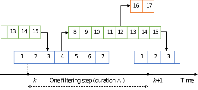
A summary of the proposed distributed PHD filter algorithm is given in Algorithm 1. Two noteworthy aspects are that (i) thefiltering operations 1 and 2 do not require or change the previous particle weights, and (ii) the fusion-related operations 8–15 do not change the current particles. As a consequence, the filtering operations 1 and 2 for time $k\hskip-0.85358pt+\!1$ can be carried out in parallel (simultaneously) with the fusion-related operations 8–15 for time $k$ . More specifically, operations 1 and 2 for time $k\hskip-0.85358pt+\!1$ can be carried out as soon as operation 7 for time $k$ is done; they do not need to wait for the results of operations 8–17. Also, operations 8–10 for time $k$ can be performed inparallel with operations 5–7 for time $k$ . In summary, the filtering operations 1 and 2 for time $k+1$ and the filtering operations 5–7 for time $k$ can be performed in parallel with the fusion-related operations 8–15 for time $k$ . Since operation 2 (including calculation of $g_{s,k}\big(\mathbf{z}\big|\mathbf{x}_{s,k}^{(j)}\big)$ ) and operation 7 (resampling) are the most computationally intensive filtering operations, a large degree of parallelization is possible. A timing diagram illustrating the scheduling and parallelization of the various operations is given in Fig. 1.

This parallelization, which is enabled by our IS method for GM–particles conversion, is an important advantage of the proposed distributed PHD filter algorithm. Indeed, with most other distributed PHD filtering algorithms, the filtering operations can only be scheduled before or after the dissemination/fusion operations. Because the time duration $\Delta$ of one filtering step (corresponding to one time step $k\to k+1$ ) is limited by the time between two sensing scans, this serial schedule implies a strong limitation of the number $I$ of dissemination/fusion iterations that can be carried out in each filtering step. More specifically, for any distributed filtering algorithm, the maximum possible value of $I$ is

I_{\text{max}}=\bigg\lfloor\frac{\Delta\hskip-0.85358pt-\hskip-0.85358ptt_{\text{filt}}\hskip-0.85358pt-\hskip-0.85358ptt_{\text{inter}}}{\tau}\bigg\rfloor\hskip 0.85358pt.

(36)

Here, $t_{\text{filt}}$ is the total time duration of all the filtering operations that cannot be carried out in parallel with the dissemination/fusion iterations; $t_{\text{inter}}$ is the time required by operations interfacing the dissemination/fusion scheme with the local filtering (preparing data to be communicated, inserting the communicated data into the local filter, etc.), which have to beperformed before and/or after the dissemination/fusion iterations; and $\tau$ is the time duration of one dissemination/fusion iteration. With our algorithm, operations 3 and 4 contribute to $t_{\text{filt}}$ and operations 8–10 and 13–15 contribute to $t_{\text{inter}}$ . Here, $t_{\text{inter}}$ is comparable to most other algorithms but $t_{\text{filt}}$ is significantly smaller. In fact, for most other algorithms, $t_{\text{filt}}$ is thetotal duration of all the filtering operations (cf. our operations 1–7), which includes also the computationally intensive likelihood calculation (cf. operation 2) and, for, a particle-based implementation, also resampling (cf. operation 7). Thus, it follows from (36) that for our algorithm, $I_{\text{max}}$ is significantly larger than for the other algorithms. This is an important advantage, as more dissemination/fusion iterations usually implya better estimation accuracy.

Refer to caption — Fig. 1: Parallelization of the operations of Algorithm 1. The numbers shown equal the operation numbers used in Algorithm 1. We note that the temporal duration of operations 11 and 12 is proportional to the number $I$ of dissemination/fusion iterations, which is upper bounded by $I_{\text{max}}$ in (36).

IX-B Communication Cost

In one dissemination/fusion iteration of the proposed distributed PHD filter, each sensor $s$ broadcasts to its neighbors a certain number of GC parameter sets, where each set consists of a weight, a $d$ -dimensional mean vector, and a $d\times d$ symmetric covariance matrix. Thus, for each GC, $n_{\textrm{GC}}\triangleq 1+d+\frac{d(d+1)}{2}$ real values are broadcast by sensor $s$ . In addition, sensor $s$ broadcasts one cardinality estimate, which is a single real value. Let $n_{s,k}^{[i]}$ denote the number of GCs contained in the GM of sensor $s$ in dissemination/fusion iteration $i$ , before the fusion with the neighboring sensors is performed. Then the total number of real values broadcast by sensor $s$ in one dissemination/fusion iteration is

N_{s,k}^{\text{com\hskip 0.85358pt[i]}}=n_{s,k}^{[i]}n_{\textrm{GC}}+1=n_{s,k}^{[i]}\bigg(1+d+\frac{d(d+1)}{2}\bigg)+1.

(37)

Note that $N_{s,k}^{\text{com\hskip 0.85358pt[i]}}$ grows linearly with the number of GCs, $n_{s,k}^{[i]}$ , and quadratically with the dimension of the target states, $d$ , and it does not depend on the number of sensors, $S$ . The last fact implies that the total communication cost for the entire network grows linearly with the network size $S$ .

While expression (37) holds for both the GM flooding scheme of Section VI-A and the GM average consensus scheme of Section VI-B, the communication costs of the two schemes are actually very different. In the case of the GM flooding scheme, the number of GCs broadcast is $n_{s,k}^{[i]}\!=\!\big|\mathcal{G}_{s,k}^{\text{F}[i-1]}\big|$ , which systematically grows with the iteration index $i$ according to (18) or equivalently (21). In the case of the GM average consensus scheme, we have $n_{s,k}^{[i]}\!=\!\big|\mathcal{G}_{s,k}^{[i-1]}\big|$ , which, according to Section VI-B, does not systematically grow with $i$ because in each iteration a GC merging step is carried out. A quantitative characterization of $\big|\mathcal{G}_{s,k}^{[i-1]}\big|$ is difficult because the reduction of the number of GCs due to merging is larger if the GCs are closer to each other.

X Simulation Study

X-A Simulation Setup

X-A1 Targets and Sensors

We simulated six targets that move in a square two-dimensional (2-D) region of interest (ROI) given by $[-1000\hskip 0.85358pt\text{m},1000\hskip 0.85358pt\text{m}]\times[-1000\hskip 0.85358pt\text{m},1000\hskip 0.85358pt\text{m}]$ . The sensor network—consisting of 16 sensors—and the target trajectories are depicted in Fig. 2. The target states consist of 2-D position and 2-D velocity, i.e., $\mathbf{x}_{k}=[x_{k}\;\dot{x}_{k}\;y_{k}\;\dot{y}_{k}]^{\text{T}}\hskip-0.85358pt$ . The target survival probability is $p_{k}^{\text{S}}(\mathbf{x}_{k-1})\!=\!0.98$ . The states of the surviving targets evolve independently according to a nearly constant velocity model, i.e., $\mathbf{x}_{k}\hskip-0.85358pt=\hskip-0.85358pt\mathbf{F}\mathbf{x}_{k-1}\hskip-0.85358pt+\mathbf{G}\mathbf{u}_{k}$ , where $\mathbf{F}\!\in\!\mathbb{R}^{4\times 4}\hskip-0.85358pt$ and $\mathbf{G}\!\in\!\mathbb{R}^{4\times 2}\hskip-0.85358pt$ are as given in [43, Eq. (14)] with sampling period $\Delta\!=\!1\hskip 0.85358pt$ s and $\mathbf{u}_{k}$ is an independent and identically distributed (iid), zero-mean, Gaussian system process with standard deviation $5\hskip 0.85358pt$ m/s². The birth intensity function is $\gamma_{k}(\mathbf{x}_{k})=0.05\cdot\mathcal{N}(\mathbf{x}_{k};\mathbf{m}_{1},\mathbf{Q})+0.05\cdot\mathcal{N}(\mathbf{x}_{k};\mathbf{m}_{2},\mathbf{Q})$ , where $\mathbf{m}_{1}\!=[{500}\hskip 0.85358pt\text{m}\;{-20}\hskip 0.85358pt\text{m}/\text{s}\;{-800}\hskip 0.85358pt\text{m}\;30\hskip 0.85358pt\text{m}/\text{s}]^{\text{T}}\hskip-0.85358pt$ , $\mathbf{m}_{2}\!=\hskip-0.85358pt[{-800}\hskip 0.85358pt\text{m}\;30\hskip 0.85358pt\text{m}/\text{s}$ ${950}\hskip 0.85358pt\text{m}\;{-30}\hskip 0.85358pt\text{m}/\text{s}]^{\text{T}}\hskip-0.85358pt$ , and $\mathbf{Q}\hskip-0.85358pt=\hskip-0.85358pt\text{diag}\{400\hskip 0.85358pt\text{m}^{2}\hskip-0.85358pt,100\hskip 0.85358pt\text{m}^{2}/\text{s}^{2}\hskip-0.85358pt,400\hskip 0.85358pt\text{m}^{2}\hskip-0.85358pt,$ $100\text{m}^{2}/\text{s}^{2}\}$ .

Eight of the 16 sensors acquire noisy position measurements within the ROI with a fixed detection probability $p_{s,k}^{\text{D}}(\mathbf{x}_{k})\hskip-0.85358pt=0.9$ . For these “linear” sensors, the measurement model

\mathbf{z}_{s,k}=[x_{k}\;y_{k}]^{\textrm{T}}+\big[v_{s,k}^{(1)}\;\hskip 0.85358ptv_{s,k}^{(2)}\big]^{\textrm{T}}\hskip-0.85358pt,\vskip-2.84526pt

where $v_{s,k}^{(1)}$ and $v_{s,k}^{(2)}$ are iid zero-mean Gaussian with standard deviation $20\hskip 0.85358pt$ m². The other eight sensors are “nonlinear” sensors that acquire noisy range and bearing measurements with detection probability given by [44]

p_{s,k}^{\text{D}}(\mathbf{x}_{k})=0.95\cdot\frac{\mathcal{N}\big(\bm{\mu}_{\mathrm{D}}(\mathbf{x}_{k});\mathbf{0},6000^{2}\mathbf{I}_{2}\big)}{\mathcal{N}(\mathbf{0};\mathbf{0},6000^{2}\mathbf{I}_{2})}\hskip 0.85358pt.\vskip-1.42262pt

Here, $\bm{\mu}_{\mathrm{D}}(\mathbf{x}_{k})\hskip-0.85358pt\triangleq\hskip-0.85358pt\big[\hskip 0.85358pt|x_{k}\!-\!x^{(s)}|\;\hskip 0.85358pt|y_{k}\!-\!y^{(s)}|\hskip 0.85358pt\big]^{\text{T}}\!$ , where $x^{(s)}$ and $y^{(s)}$ are the coordinates of sensor $s$ . The range-bearing measurement model is

\mathbf{z}_{s,k}=\begin{bmatrix}\sqrt{(x_{k}\!-\!x^{(s)})^{2}+(y_{k}\!-\!y^{(s)})^{2}}\,\,\\[1.42262pt] \tan^{-1}\!\Big(\frac{x_{k}-x^{(s)}}{y_{k}-y^{(s)}}\Big)\end{bmatrix}+\begin{bmatrix}v_{s,k}^{(1)}\\[4.2679pt] v_{s,k}^{(2)}\end{bmatrix}\hskip-0.85358pt,\vskip-1.99168pt

where $v_{s,k}^{(1)}$ and $v_{s,k}^{(2)}$ are, individually, iid zero-mean Gaussian with standard deviation $\sigma_{1}\!=\!20\hskip 0.85358pt$ m and $\sigma_{2}\hskip-0.85358pt=\hskip-0.85358pt(\pi/90)\hskip 0.85358pt$ rad, respectively. The field of view of the nonlinear sensors is a discof radius 3000m centered at the sensor position; this disc always covers the entire ROI. For both the linear and the nonlinear sensors, clutter is uniformly distributed over the sensor’s field of view with an average number of ten clutter measurements per time step, or equivalently clutter intensity $\kappa_{s,k}(\mathbf{z}_{k})$ $=\hskip-0.85358pt10/(2000^{2})\hskip-0.85358pt=\hskip-0.85358pt2.5\cdot 10^{-6}$ for the linear sensors and $\kappa_{s,k}(\mathbf{z}_{k})$ $=\hskip-0.85358pt10/(2\pi\hskip-0.85358pt\cdot\hskip-0.85358pt3000)\approx 5.31\cdot 10^{-4}$ for the nonlinear sensors. The clutter measurements of different sensors are independent.

X-A2 Local PHD Filters

We consider two scenarios. In the first scenario, all the local PHD filters use a particle-based implementation. In the second scenario, only the local PHD filters at the nonlinear sensor nodes use a particle-based implementation, whereas the local PHD filters at the linear sensor nodes use a GM-based implementation [3, 10]. The results for the second scenario demonstrate the applicability of our distributed PHD filter in heterogeneous networks combining particle-based and GM-based local PHD filters.

We compare the performance and computing time of the following particle-based PHD

filters:

•

The proposed distributed PHD filter, which will be briefly referred to as AA-F-IS or AA-C-IS depending on whether flooding (F) or average consensus (C) is used as the dissemination/fusion scheme.
•

A modified version of the GA fusion-based, particle-based, distributed PHD filter proposed in [12], briefly referred to as GA-EMD. In [12], two important steps are(i) a conversion of the particle representation of the PHDinto a kernel-based representation, and (ii) the construction of the multitarget exponential mixture density (EMD). Regarding the first step, we replaced the clustering algorithm for kernel function learning proposed in [12]—which we observed in our simulations to be computationally intensive and potentially unstable—with our particles-GM conversion algorithm from Section V. Regarding the second step, we use our IS method for GM-particles conversion (see Section VII) for updating the fused particles. Finally, we do not employ the sophisticated strategy for online adjustment of the fusion weights proposed in [12] but use fixed Metropolis weights, which have been widely used for GA-based GM-PHD fusion [4].

The resulting modification of the EMD fusion method of [12] is more computationally efficient, although—as shown later—it is still considerably less efficient than our proposed fusion method. Moreover, just as the filter of [12], it has a significantly higher communication costbecause it communicates both the particles and the kernel/GM parameters. For this reason, using flooding for dissemination/fusion is infeasible, and hence we only use the average consensus scheme.

Fig. 3: Results for the first scenario: (a) Network OSPA error versus time $k$ (here, the distributed filters use $I\!=\!5$ dissemination/fusion iterations). (b) Time-averaged network OSPA error versus number of dissemination/fusion iterations $I$ . (c) Average communication cost versus $I$ .
•

A modified version of our proposed distributed PHD filter, in which the GM–particles conversion is done via the standard sampling (SS) method—i.e., sampling directly from the fused GM-PHD $D_{s,k}^{\text{GM}[I]}(\mathbf{x})$ —instead of our IS method from Section VII. We consider this filter to compare the IS method with the SS method. We refer to it as AA-F-SS or AA-C-SS depending on the dissemination/fusion scheme employed.
•

A noncooperative PHD filter in which each local PHD filter relies solely on its own local measurements and does not communicate with other local PHD filters.

The local PHD filters use systematic resampling [42], andthey adjust the number of particles via resampling to be $200\cdot\hskip-0.85358pt\hat{N}_{s,k}^{\text{local}}$ if $\hat{N}_{s,k}^{\text{local}}\!\geq\hskip-0.85358pt0.5$ and 100 otherwise, where $\hat{N}_{s,k}^{\text{local}}\hskip-0.85358pt=\mathrm{round}\{W_{s,k}\}$ . (Here, we use $W_{s,k}$ and not $W_{\!s,k}^{[I]}$ because in the resampling step, $W_{\!s,k}^{[I]}$ is not available yet.)

The target state estimates $\hat{\mathbf{x}}_{k}^{(\nu)}$ are calculated as described in Section VIII-B. The threshold defining $\Omega_{s,k}(\mathbf{z})$ (see Section V) is $T_{\Omega}\!=\hskip-0.85358pt0.3$ . The consensus-based filters (AA-C-SS/IS and GA-EMD) perform GC merging in each consensus iteration (see Section VI-B); GCs are merged if their Mahalanobis distance is smaller than 2 [40].

For each of the two scenarios, we performed 100 simulation runs using the target trajectories shown in Fig. 2 and randomly generated measurement noise and initial particles. Each simulation run consists of 80 time steps.

X-B First Scenario—Particle-based Local PHD Filters

In the first scenario, all the local PHD filters use a particle-based implementation.

X-B1 Tracking Accuracy

We quantify the target detection and position estimation performance of the filters by the mean optimal subpattern assignment (OSPA) error [45] with cutoff parameter $c\hskip-0.85358pt=\!1000\hskip 0.85358pt$ m and order $p\hskip-0.85358pt=\hskip-0.85358pt2$ . More specifically, we consider the average of the OSPA errors obtained by all the sensors, referred to as network OSPA error (briefely N-OSPA) and the average of the network OSPA errors over all the 80 time steps, referred to as time-averaged network OSPA error (TN-OSPA). Fig. 3(a) shows the N-OSPA of the distributed PHD filters using $I\!=\!5$ dissemination/fusion iterations, as well as of the noncooperative PHD filter, versus time $k$ . Fig. 3(b) shows the TN-OSPA versus the number $I$ of dissemination/fusion iterations. One can see that the D-PHD filters have a significantly smaller OSPA error than the noncooperative PHD filter.

According to Fig. 3(b), the reduction of the TN-OSPA for growing $I$ is quite fast initially. For larger $I$ , the TN-OSPA decreases more slowly (in the case of the consensus-based filters) or it stays roughly constant (in the case of the flooding-based filters), or it even starts increasing again (in the case of GA-EMD). Regarding the flooding-based filters, we recall from Section VI-A that the flooding dissemination of the GM parameters is already complete when $I$ equals the network diameter $R\hskip-0.85358pt=\hskip-0.85358pt5$ , and thus no further gains can be achieved for $I\hskip-0.85358pt\geq\hskip-0.85358pt6$ . Furthermore, we conjecture that the increase of the TN-OSPA of GA-EMD for $I\hskip-0.85358pt\geq\hskip-0.85358pt7$ is due to the fact that a missed detection at any single sensor can degrade the performance of GA fusion significantly, and the probability of such a missed detection increases when more sensors are involved. We note that a similar increase of the OSPA for additional GA dissemination/fusion iterations was reported in [5, Fig. 8] (in the intervals $k\!\in\![25\hskip 0.85358pt\text{s},100\hskip 0.85358pt\text{s}]$ and $k\!\in\![790\hskip 0.85358pt\text{s},800\hskip 0.85358pt\text{s}]$ ). It is furthermore seen in Fig. 3(b) that the TN-OSPA of GA-EMD is larger than that of AA-C-IS/SS (except for $I\!=\!1$ , where according to Fig. 3(b) it is slightly smaller than that of AA-C-IS).

The OSPA performance of the SS-based filters (AA-F-SSand AA-C-SS) is seen to be better than that of the corresponding IS-based filters (AA-F-IS and AA-C-IS, respectively). This is because sampling directly from $D_{s,k}^{\text{GM}[I]}(\mathbf{x})$ represents $D_{s,k}^{\text{GM}[I]}(\mathbf{x})$ more accurately than the indirect sampling performed by our IS method. (However, we recall that the IS method enables the far-reaching parallelization of filtering and fusion operations described in Section IX-A.) Finally, the consensus-based filters (AA-C-SS and AA-C-IS) outperform the flooding-based filters (AA-F-SS and AA-F-IS, respectively); the only exception is $I\!=\!1$ , where the consensus and flooding schemes differ merely by the choice of the fusion weights (uniform and Metropolis weights, respectively). This superiority of the GM consensus scheme (for $I\hskip-0.85358pt\geq\hskip-0.85358pt2$ ) is unexpected, since flooding yields a faster dissemination of the GM parameters than consensus. A possible reason is the GC merging performed by the GM consensus scheme in each fusion iteration. In this context, an interesting observation is that GA-EMD—which is also consensus-based and performs GC merging—outperforms AA-F-IS for $3\!\leq\!I\!\leq\!9$ . In additional simulations for various scenarios, we observed that the performance of consensus-based PHD filter algorithms with GC merging, including AA-C-SS/IS and GA-EMD, is highly sensitive to the threshold of the Mahalanobis distance used for GC merging: we found that threshold 2 yields the best filter performance, whereas other thresholds can lead to a significantly poorer performance.

X-B2 Communication Cost

We measure the average communication cost (ACC) of the various filters by the number of real values broadcast by a sensor to its neighbors during all the dissemination/fusion iterations performed at one time step, averaged over all the sensors, time steps, and simulation runs. Note that in addition to one real value for the cardinality estimate, only GC parameters are broadcast in AA-F/C-IS and AA-F/C-SS whereas in GA-EMD, both GC parameters and unweighted particles (i.e., the particles after the resampling step) are broadcast. Here, each unweighted particle amounts to four real values.

Fig. 3(c) shows the ACC versus $I$ . The increase of the ACCof GA-EMD and AA-C-IS/SS with $I$ is an expected result because the ACC was defined as the average total communication cost for all the $I$ dissemination/fusion iterations. The ACC of AA-F-IS/SS increases up to $I\!=\!5$ but stays constant afterwards. This is also expected because, as mentioned earlier, the flooding dissemination is already complete when $I\!=\!R\hskip-0.85358pt=\hskip-0.85358pt5$ , and thus no additional information needs to be communicated for $I\hskip-0.85358pt\geq\hskip-0.85358pt6$ . The ACC of GA-EMD is seen to be larger by about one order of magnitude than that of the other filters; this is because GA-EMD communicates a large number of particles in addition to GC parameters. Furthermore, the ACC of the flooding-based filters is larger than that of the consensus-based filters for $I$ between 2 and 5, and smaller for $I\geq 7$ . At this point, we recall from Section IX-B that the communication cost of the consensus-based filters strongly depends on the GC merging. Using a larger threshold for the Mahalanobis distance (so that more GCs are merged) would result in a smaller communication cost but also in a poorer tracking accuracy. Finally, AA-F-SS and AA-F-IS are seen to have almost the same ACC, and similarly for AA-C-SS and AA-C-IS. This is because the choice of the GM–particles conversion method—SS or IS—has only little effect on the communication cost.

TABLE I: Results for the first scenario: Average computing time of one filtering step. The distributed filters use

I\!=\!5

dissemination/ fusion iterations.

Filter	Average Computing Time [s]
Noncooperative	0.079
AA-F-SS	0.181
AA-C-SS	0.347
AA-C-IS	0.387
AA-F-IS	0.558
GA-EMD	1.837

X-B3 Computational Complexity

Finally, we quantify the computational complexity of the various filters by the average computing time of each filtering step (corresponding to each time step $k\to k\hskip-0.85358pt+\!1$ ), where the averaging is over all the local PHD filters, time steps, and simulation runs. The computing times were obtained using MATLAB implementations on an Intel Core M-5Y71 CPU. Table I shows the average computing time for the distributed PHD filters using $I\!=\!5$ dissemination/fusion iterations, as well as for the noncooperative PHD filter, versus time $k$ . It is seen that GA-EMD is significantly more complex than the other distributed filters. Furthermore, AA-F-IS and AA-C-IS are more complex than AA-F-SS and AA-C-SS; this is because the IS method is more complex than the SS method. AA-F-IS is more complex than AA-C-IS, due to the larger number of GCs that are processed. Indeed, in AA-C-IS, the number of GCs is reduced by GC merging, and the complexity of the GM merging operations is considerably smaller than the added complexity of AA-F-IS caused by the additional GCs. On the other hand, AA-F-SS is less complex than AA-C-SS. Here, the reason is that the SS method employed by AA-F-SS and AA-C-SS has a low complexity, and thus the complexity of the merging operations performed by AA-C-SS is larger than the added complexity of AA-F-SS caused by the additional GCs.

X-C Second Scenario—Particle-based and GM-based Local PHD Filters

Next, we study a heterogeneous network where the eight nonlinear sensor nodes use a particle-based local PHD filter and the eight linear sensor nodes use a GM-based local PHD filter [3, 10] (briefly referred to as GM-PHD filter). The sensor network topology and the target trajectories are as before (see Fig. 2). The GM-PHD filters use at most 100 GCs. For mixture reduction, following [3], they remove GCs with a weight smaller than $10^{-4}$ and merge GCs with a Mahalanobis distance smaller than 4. (We note that here, the Mahalanobis distance threshold 4 performed better than the threshold 2 thatwe used in the consensus-based particle-PHD filters in Section X-B.) Furthermore, for fusing their local GM with the GMs of the other sensors, the GM-PHD filters perform a straightforward union of the GM parameter sets and subsequently adjust the weights using the cardinality averaging method discussed in Section VIII-A. The combination—within the sensor network—of the GM-PHD filters with the particle-based AA-F/C-SS/IS filters will be briefly referred to as “AA-F/C-SS/IS.” We no longer consider GA-EMD as it cannot becombined with a GM-PHD filter in a straightforward fashion (i.e., without conversions between particle and GM representations).

The simulation results for this scenario, shown in Fig. 4 and Table II, are generally similar to those for the first scenario (see Fig. 3 and Table I). A difference is that now AA-F-IS and AA-F-SS have a smaller TN-OSPA than, respectively, AA-C-IS and AA-C-SS for $I\!\leq\hskip-0.85358pt4$ , instead of only for $I\!=\!1$ (as was the case in the first scenario). This is because now half of the local filters are GM-PHD filters, for which flooding-based fusion performs better than consensus-based fusion [10].

TABLE II: Results for the second scenario: Average computing time of one filtering step. The distributed filters use

I\!=\!5

dissemination/fusion iterations.

Filter	Average Computing Time [s]
Noncooperative	0.096
AA-F-SS	0.233
AA-C-SS	0.353
AA-C-IS	0.381
AA-F-IS	0.422

XI Conclusion

We proposed a distributed PHD (D-PHD) filter where the local filters use a particle-based implementation to support nonlinear/non-Gaussian system models, but the fusion of the local PHDs is based on a Gaussian mixture (GM) representation to reduce communication and enable an easy combination with GM-based local filters. Our D-PHD filter differs from most existing filters in that it seeks to compute the arithmetic average (AA) of the local PHDs, rather than the geometric average (GA). Two noteworthy components of ourD-PHD filter algorithm are (i) a “significance-based” method for converting particle representations into GM representations, which reduces communication and complexity, and (ii) an importance sampling method for converting the fused GMs into particle representations, which enables a parallelization of filtering and fusion operations. This parallelization is especially advantageous when the sensing rate is high and/or the duration of one dissemination/fusion iteration is large.

An experimental comparison of our filter with a state-of-the-art filter using GA fusion showed that, in the considered scenarios, consensus-based AA fusion outperforms consensus-based GA fusion in terms of estimation accuracy, complexity, and communication cost. Our simulations also showed that consensus-based AA fusion can outperform flooding-based AA fusion in terms of both estimation accuracy and communication cost. We expect that this advantage of AA fusion can to be further increased by using more sophisticated mixture reduction schemes such as [46, 47].

Appendix A Proof of Eq. (31)

To show that the choice of $P_{j^{\prime}}$ in (31) yields (30), we note that $N_{s,k}^{(j^{\prime})}$ can be written as $N_{s,k}^{(j^{\prime})}\!=\hskip-0.85358pt\sum_{j=1}^{\tilde{J}_{s,k}}I\big[\tilde{\mathbf{x}}_{s,k}^{(j)}\!=\hskip-0.85358pt\mathbf{x}_{s,k}^{(j^{\prime})}\big]$ , where $I\big[\tilde{\mathbf{x}}_{s,k}^{(j)}\!=\hskip-0.85358pt\mathbf{x}_{s,k}^{(j^{\prime})}\big]$ equals $1$ if $\tilde{\mathbf{x}}_{s,k}^{(j)}\!=\hskip-0.85358pt\mathbf{x}_{s,k}^{(j^{\prime})}$ and $0$ otherwise. Thus,

\mathrm{E}\big[N_{s,k}^{(j^{\prime})}\big|\xi_{s,k}\big]=\sum_{j=1}^{\tilde{J}_{s,k}}\mathrm{E}\big[I\big[\tilde{\mathbf{x}}_{s,k}^{(j)}\!=\hskip-0.85358pt\mathbf{x}_{s,k}^{(j^{\prime})}\big]\big|\xi_{s,k}\big]\hskip 0.85358pt.\vskip-5.69054pt

(38)

Now

		$\displaystyle\mathrm{E}\big[I\big[\tilde{\mathbf{x}}_{s,k}^{(j)}\!=\hskip-0.85358pt\mathbf{x}_{s,k}^{(j^{\prime})}\big]\big\|\xi_{s,k}\big]$
		$\displaystyle\;\;=1\cdot\mathrm{Pr}\big[\tilde{\mathbf{x}}_{s,k}^{(j)}\!=\hskip-0.85358pt\mathbf{x}_{s,k}^{(j^{\prime})}\big\|\xi_{s,k}\big]+0\cdot\mathrm{Pr}\big[\tilde{\mathbf{x}}_{s,k}^{(j)}\!\not=\hskip-0.85358pt\mathbf{x}_{s,k}^{(j^{\prime})}\big\|\xi_{s,k}\big]$
		$\displaystyle\;\;=P_{j^{\prime}}\hskip 0.85358pt,$

whence (38)

becomes

	$\displaystyle\mathrm{E}\big[N_{s,k}^{(j^{\prime})}\big\|\xi_{s,k}\big]$	$\displaystyle=\sum_{j=1}^{\tilde{J}_{s,k}}P_{j^{\prime}}$
		$\displaystyle=\tilde{J}_{s,k}\hskip 0.85358ptP_{j^{\prime}}$
		$\displaystyle=\mathrm{round}\{N_{\textrm{p}}\hskip 0.85358ptW_{s,k}\}\hskip 0.85358ptP_{j^{\prime}}$
		$\displaystyle\approx N_{\textrm{p}}\hskip 0.85358ptW_{s,k}\hskip 0.85358ptP_{j^{\prime}}$
		$\displaystyle=N_{\textrm{p}}\hskip 0.85358ptw_{s,k}^{(j^{\prime})},$

where (29) and (31) have been used. Hence, to within a rounding error (caused by replacing $\mathrm{round}\{N_{\textrm{p}}\hskip 0.85358ptW_{s,k}\}$ with $N_{\textrm{p}}\hskip 0.85358ptW_{s,k}$ ), $\mathrm{E}\big[N_{s,k}^{(j^{\prime})}\big|\xi_{s,k}\big]$ equals $N_{\textrm{p}}\hskip 0.85358ptw_{s,k}^{(j^{\prime})}$ , as postulated in (30).

References

[1] R. P. S. Mahler, “Multitarget Bayes filtering via first-order multitarget moments,” IEEE Trans. Aerosp. Electron. Syst., vol. 39, no. 4, pp. 1152–1178, Oct. 2003.
[2] B.-N. Vo, S. Singh, and A. Doucet, “Sequential Monte Carlo methods for multitarget filtering with random finite sets,” IEEE Trans. Aerosp. Electron. Syst., vol. 41, no. 4, pp. 1224–1245, Oct. 2005.
[3] B.-N. Vo and W. K. Ma, “The Gaussian mixture probability hypothesis density filter,” IEEE Trans. Signal Process., vol. 54, no. 11, pp. 4091–4104, Nov. 2006.
[4] G. Battistelli, L. Chisci, C. Fantacci, A. Farina, and A. Graziano, “Consensus CPHD filter for distributed multitarget tracking,” IEEE J. Sel. Topics Signal Process, vol. 7, no. 3, pp. 508–520, Jun. 2013.
[5] G. Battistelli, L. Chisci, C. Fantacci, A. Farina, and R. P. S. Mahler, “Distributed fusion of multitarget densities and consensus PHD/CPHD filters,” in Proc. SPIE, vol. 9474, 2015, pp. 94 740E–94 740E–15.
[6] M. Gunay, U. Orguner, and M. Demirekler, “Chernoff fusion of Gaussian mixtures based on sigma-point approximation,” IEEE Trans. Aerosp. Electron. Syst., vol. 52, no. 6, pp. 2732–2746, Dec. 2016.
[7] W. Yi, M. Jiang, S. Li, and B. Wang, “Distributed sensor fusion for RFS density with consideration of limited sensing ability,” in Proc. FUSION 2017, Xi’an, China, Jul. 2017.
[8] J. Y. Yu, M. Coates, and M. Rabbat, “Distributed multi-sensor CPHD filter using pairwise gossiping,” in Proc. IEEE ICASSP 2016, Shanghai, China, Mar. 2016, pp. 3176–3180.
[9] T. Li, J. Corchado, and S. Sun, “On generalized covariance intersection for distributed PHD filtering and a simple but better alternative,” in Proc. FUSION 2017, Xi’an, China, Jul. 2017, pp. 808–815.
[10] ——, “Partial consensus and conservative fusion of Gaussian mixtures for distributed PHD fusion,” IEEE Trans. Aerosp. Electron. Syst., 2018, to be published.
[11] M. Üney, S. Julier, D. Clark, and B. Ristić, “Monte Carlo realisation of a distributed multi-object fusion algorithm,” in Proc. SSPD 2010, London, UK, Sep. 2010.
[12] M. Üney, D. E. Clark, and S. J. Julier, “Distributed fusion of PHD filters via exponential mixture densities,” IEEE J. Sel. Topics Signal Process, vol. 7, no. 3, pp. 521–531, Jun. 2013.
[13] A. K. Gostar, R. Hoseinnezhad, and A. Bab-Hadiashar, “Cauchy-Schwarz divergence-based distributed fusion with Poisson random finite sets,” in Proc. ICCAIS 2017, Chiang Mai, Thailand, Oct. 2017, pp. 112–116.
[14] T. Li, V. Elvira, H. Fan, and J. M. Corchado, “Local diffusion-based distributed SMC-PHD filtering using sensors with limited sensing range,” IEEE Sensors J., 2018, to be published.
[15] J. K. Uhlmann, “Dynamic map building and localization: New theoretical foundations,” Ph.D. dissertation, University of Oxford, UK, 1995.
[16] S. Julier and J. Uhlmann, “General decentralized data fusion with covariance intersection (CI),” in Handbook of Data Fusion, D. Hall and J. Llinas, Eds. Boca Raton, FL, USA: CRC Press, 2001, ch. 12, pp. 1–25.
[17] T. Bailey, S. Julier, and G. Agamennoni, “On conservative fusion of information with unknown non-Gaussian dependence,” in Proc. FUSION 2012, Singapore, Jul. 2012, pp. 1876–1883.
[18] R. P. S. Mahler, “Optimal/robust distributed data fusion: A unified approach,” in Proc. SPIE, vol. 4052, 2000, pp. 128–138.
[19] D. Clark, S. Julier, R. Mahler, and B. Ristic, “Robust multi-object sensor fusion with unknown correlations,” in Proc. SSPD 2010, London, UK, Sep. 2010.
[20] R. P. S. Mahler, “Toward a theoretical foundation for distributed fusion,” in Distributed Data Fusion for Network-Centric Operations, D. Hall, C.-Y. Chong, J. Llinas, and M. Liggins, Eds. Boca Raton, FL, USA: CRC Press, 2012, pp. 199–224.
[21] M. Üney, J. Houssineau, E. Delande, S. J. Julier, and D. E. Clark, “Fusion of finite set distributions: Pointwise consistency and global cardinality,” IEEE Trans. Aerosp. Electron. Syst., 2018, to be published.
[22] R. L. Streit, “Multisensor multitarget intensity filter,” in Proc. FUSION 2008, Cologne, Germany, Jun. 2008.
[23] L. Zhao, P. Ma, X. Su, and H. Zhang, “A new multi-target state estimation algorithm for PHD particle filter,” in Proc. FUSION 2010, Edinburgh, Scotland, UK, Jul. 2010.
[24] B. Ristic, D. Clark, and B.-N. Vo, “Improved SMC implementation of the PHD filter,” in Proc. FUSION 2010, Edinburgh, Scotland, UK, Jul. 2010.
[25] M. Schikora, W. Koch, R. Streit, and D. Cremers, “Sequential Monte Carlo method for multi-target tracking with the intensity filter,” in Advances in Intelligent Signal Processing and Data Mining: Theory and Applications, P. Georgieva, L. Mihaylova, and L. C. Jain, Eds. Heidelberg, Germany: Springer, 2012, ch. 4, pp. 55–87.
[26] C. P. Robert and G. Casella, Monte Carlo Statistical Methods. Secaucus, NJ, USA: Springer, 2005.
[27] R. P. S. Mahler, Statistical Multisource-Multitarget Information Fusion. Norwood, MA, USA: Artech House, 2007.
[28] S. S. Singh, B.-N. Vo, A. Baddeley, and S. Zuyev, “Filters for spatial point processes,” SIAM J. Contr. Opt., vol. 48, no. 4, pp. 2275–2295, 2009.
[29] S. M. Kay, Fundamentals of Statistical Signal Processing: Estimation Theory. Upper Saddle River, NJ, USA: Prentice-Hall, 1993.
[30] H. G. Hoang, B.-N. Vo, B.-T. Vo, and R. Mahler, “The Cauchy-Schwarz divergence for Poisson point processes,” IEEE Trans. Inf. Theory, vol. 61, no. 8, pp. 4475–4485, Aug. 2015.
[31] T. Li, F. Hlawatsch, and P. M. Djuríc, “Cardinality-consensus-based PHD filtering for distributed multitarget tracking,” IEEE Signal Process. Lett., vol. 26, no. 1, pp. 49–53, Jan. 2019.
[32] M. Coates, “Distributed particle filters for sensor networks,” in Proc. IPSN 2004, New York, NY, USA, Apr. 2004, pp. 99–107.
[33] X. Sheng, Y. H. Hu, and P. Ramanathan, “Distributed particle filter with GMM approximation for multiple targets localization and tracking in wireless sensor network,” in Proc. IPSN 2005, Los Angeles, California, CA, USA, Apr. 2005, pp. 181–188.
[34] D. Gu, “Distributed particle filter for target tracking,” in Proc. IEEE ICRA 2007, Rome, Italy, Apr. 2007, pp. 3856–3861.
[35] O. Hlinka, F. Hlawatsch, and P. M. Djuric, “Distributed particle filtering in agent networks: A survey, classification, and comparison,” IEEE Signal Process. Mag., vol. 30, no. 1, pp. 61–81, Jan. 2013.
[36] T. Li, J. Corchado, and J. Prieto, “Convergence of distributed flooding and its application for distributed Bayesian filtering,” IEEE Trans. Signal Inf. Process. Netw., vol. 3, no. 3, pp. 580–591, Sep. 2017.
[37] J. Li and A. Nehorai, “Distributed particle filtering via optimal fusion of Gaussian mixtures,” IEEE Trans. Signal Inf. Process. Netw., vol. 4, no. 2, pp. 280–292, Jun. 2018.
[38] R. Olfati-Saber, J. A. Fax, and R. M. Murray, “Consensus and cooperation in networked multi-agent systems,” Proc. IEEE, vol. 95, no. 1, pp. 215–233, Jan. 2007.
[39] L. Xiao and S. Boyd, “Fast linear iterations for distributed averaging,” Syst. Control. Lett., vol. 53, no. 1, pp. 65–78, 2004.
[40] D. J. Salmond, “Mixture reduction algorithms for target tracking in clutter,” in Proc. SPIE, vol. 1305, 1990, pp. 434–445.
[41] S. Reece and S. Roberts, “Generalised covariance union: A unified approach to hypothesis merging in tracking,” IEEE Trans. Aerosp. Electron. Syst., vol. 46, no. 1, pp. 207–221, Jan. 2010.
[42] T. Li, M. Bolić, and P. M. Djurić, “Resampling methods for particle filtering: Classification, implementation, and strategies,” IEEE Signal Process. Mag., vol. 32, no. 3, pp. 70–86, May 2015.
[43] X. R. Li and V. P. Jilkov, “Survey of maneuvering target tracking. Part I. Dynamic models,” IEEE Trans. Aerosp. Electron. Syst., vol. 39, no. 4, pp. 1333–1364, Oct. 2003.
[44] B.-T. Vo, B.-N. Vo, and A. Cantoni, “The cardinality balanced multi-target multi-Bernoulli filter and its implementations,” IEEE Trans. Signal Process., vol. 57, no. 2, pp. 409–423, Feb. 2009.
[45] D. Schuhmacher, B.-T. Vo, and B.-N. Vo, “A consistent metric for performance evaluation of multi-object filters,” IEEE Trans. Signal Process., vol. 56, no. 8, pp. 3447–3457, Aug. 2008.
[46] D. F. Crouse, P. Willett, K. Pattipati, and L. Svensson, “A look at Gaussian mixture reduction algorithms,” in Proc. FUSION 2011, Chicago, IL, USA, Jul. 2011.
[47] T. Ardeshiri, K. Granström, E. Ozkan, and U. Orguner, “Greedy reduction algorithms for mixtures of exponential family,” IEEE Signal Process. Lett., vol. 22, no. 6, pp. 676–680, Jun. 2015.