The Hubble constant from SN Refsdal
Abstract
Hubble Space Telescope observations from December 11 2015 detected the expected fifth counter image of SN Refsdal at . In this letter, we compare the time delay predictions from numerous models with the measured value derived by Kelly et al. [20] from very early data in the light curve of the SN Refsdal, and find a best value for (68% CL), in excellent agreement with predictions from CMB and recent weak lensing data + BAO + BBN (from the DES Collaboration). This is the first constraint on derived from time delays between multiple lensed SN images, and the first with a galaxy cluster lens, so subject to systematic effects different from other time-delay estimates. Additional time delay measurements from new multiply-imaged SNe will allow derivation of competitive constraints on .
Keywords:
gravitational lensing: strong — cosmology: theory — methods: statistical — galaxies: clusters: individual (MACS J1149.5+2223) — supernovae: individual (SN Refsdal)I Introduction
Galaxy clusters bend the path of photons emitted by distant objects, creating multiple images of the same background source, each with different magnification and arrival times. Time delays between multiple images of the same source depend on the cosmological model, and most notably on the Hubble constant, . The potential to constrain with multiple supernova (SN) images was first suggested by [30]. However, no multiply imaged (and resolved) SN has ever been observed until just recently. In 2014 four counter-images of the same supernova, SN Refsdal [19, 32, 20, 21], located at redshift , were found around a member galaxy in the cluster MACSJ1149.5+2223 [11, hereafter MACS1149, ] at redshift . The predicted time delay between these four images is relatively small (a few days) making them impractical to derive useful constraints on since the time delays are smaller than the accuracy with which the observed time delay can be determined. Approximately a year after the initial detection of the four supernova images, a fifth counter-image appeared, this one having a considerably longer time delay. The position and the time of reappearance were predicted by different lens models with remarkable precision [28, 34, 10, 37, 16]. This accuracy is possible since MACS1149 has been observed with unprecedented detail as part of the Hubble Frontier Fields (HFF) program. MACS1149 contains tens of identified lensed galaxies allowing for detailed modeling of the lens [13, 14, 15, 23, 40, 6, 7, 10, 18, 24, 25].
The predictions for the SN time delay were based on a set of assumptions, including the value , which was adopted by all teams in their model predictions. Since time delays are inversely proportional to , it is possible to constrain the value of directly, as originally suggested by Refsdal. The adopted value lies in between the two of the most precise published estimates. Constraints from the cosmic microwave background (CMB) points towards a low [29] while local measurements favor a high [31] instead. More recently, DES Collaboration et al. [5] combine intermediate-redshift observations—the Dark Energy Survey Year 1 clustering and weak lensing data with Baryon Acoustic Oscillations (BAO)—with Big Bang Nucleosynthesis (BBN) experiments to obtain (68% CL). The difference between intermediate/early and late-time universe cosmologies is of substantial interest. Generalizations of the dark energy phenomenology that predict an equation of state that changes after some transition time could support both results. While [5] conclude that the ensemble of data are consistent within uncertainties, additional constraints on the Hubble constant based on measurements at intermediate redshift would provide valuable clarity.
In this letter, we derive an estimate of based on the observed time delay for the SN Refsdal system and an ensemble of lens models derived by different teams that use independent reconstruction methods. Our results provide a separate geometrical inference for [22, 33, 39, 2]. Hereafter, we adopt a fiducial cosmological model with and , which is the cosmology used to infer the lens models. When re-scaling the value of the predicted time delay, the only cosmological parameter being changed is (see section II for details). Similar attempts have been made with galaxy-QSO lensing (with lensing constraints or less) but never with galaxy clusters where the number of lensing constraints can exceed one hundred. The H0LiCOW-COSMOGRAIL program [3, 36] probably represents the best effort so far to constrain with time delays from multiple lensed QSO. In their most recent work, is constrained with to within [2]. Their best inferred value of is in good agreement with the local distance ladder measurements of .
The work is organized as follows. Section II introduces the time delay formalism and describes the published time delay predictions for SN Refsdal. Section III describes the analysis performed to derive the most likely value of from the available data. Finally, sections IV and V summarize our results and conclusions.
II Hubble constant estimate from SN Refsdal time delays
The time delay with respect to an unperturbed null geodesic depends on the angular separation between the image and the source, on the lensing potential at the position of the image, and on the cosmological model through the angular diameter distances. Distances, in turn, depends on the cosmic expansion history of the universe, which is proportional to the Hubble rate,
| (1) |
where is the unlensed source position and is the lens potential at the position of the observed counter-image . The quantities , and are the angular diameter distance to the lens, to the source and between the lens and the source, respectively. These three distances are inversely proportional to , and therefore the time delay is also inversely proportional to . The factor encodes the cosmological dependency that, as shown by Bonvin et al. [2], is mostly sensitive to and depends weakly on other cosmological parameters. For instance, a change of in the cosmological parameter translates into a change of only in . Because of this weak dependence on other cosmological parameters, we consider the cosmological model fixed and vary only .
The difference in the predicted time delay between two positions in the lens plane depends on a delicate balance between the lensing potential and the relative separations. These terms are typically comparable in magnitude near the minimum of the potential. Since the term is straightforward, the uncertainties in the lensing potential are the primary source of systematic errors in the prediction of the time delays, followed by the unknown value of .
Luckily, lensing models for clusters like MACS1149 are constrained by tens of multiply-imaged lensed background galaxies with a wide range of known redshifts that reduce the uncertainties in the lens models [17, 1]. Traditional time delay measurements based on lensed quasars are based on lens models with typically just one lensed source (the QSO itself) making them more vulnerable to degeneracies like the mass-sheet degeneracy or to projection effects that can involve masses comparable to that of the lens being modeled. Model predictions for time delays are less prone to errors in regions where the number of lensing constraints are more abundant. In the case of MACS1149, the highest density of lensing constraints is found in the vicinity of the multiple supernova images. One should then expect systematics to be relatively small in the case of the SN Refsdal. Finally, the wealth of lens models and predictions for the time delay of the SN Refsdal from multiple investigators allows us to account for the statistical uncertainty in the lens model prediction. We should note however, that some systematic errors may affect all models in a similar fashion (with projection effects being a good example). This will be discussed in more detail later.
II.1 The case of SN Refsdal
The SN Refsdal [19, 32, 20, 21] was the first example of a resolved multiply imaged lensed SN. Kelly et al. [20] presents the first estimation of the relative time delay and magnification ratio of S1 (position of knot 1 in the original quadruplet image) and SX (the position at which SN Refsdal reappeared) based on the early light curve of SX. The lensing constraints from the HFF program allowed for a variety of predictions of the time delay and relative magnification of a fifth image. These predictions where made assuming a fiducial cosmological model, needed for computing the distances in Eq.1. If the fiducial model assumed the wrong this would translate into a predicted time delay that is biased with respect to the measured one. The predictions ranged from months [34] to year [10]. Similar predictions extending from months to months were later published in [37] by different teams. SN Refsdal reappeared promptly approximately one year after its first appearance. Overall, the lens models predict reasonably well the time of reappearance of SN Refsdal [20].
In table 1, we summarize the predicted time delays between SX and S1, and the magnification ratios, , as derived by the different models [37]. We also included earlier predictions made by Diego et al. [10], labeled as “Die-16". Both the models “Die-16" in [10] and “Die-a" in Treu et al. [37] were derived using the same code WSLAP+ [8, 9] and HFF data, but the model “Die-16" has higher spatial resolution (and precision) around the positions of the S1-SX counter-images. The model “Zit-g" in Treu et al. [37] was found to have numerical errors after the acceptance of that paper, affecting all the “Zit-g" predictions presented there [37, see note added in proof in]. Therefore, we do not include “Zit-g" model in the estimation of . We have incorporated only models that use data from the HFF program with a large number of constraints. Moreover, we also exclude from the analysis not truly blind predictions, such as the analytic solution for the time delay given in Jauzac et al. [16] or the updated value of “Zit-g" model (“Zitrin-c") presented in Kelly et al. [20].
| (days) | ||
|---|---|---|
| Die-16 | ||
| Die-a | ||
| Gri-g | ||
| Ogu-g | ||
| Ogu-a | ||
| Sha-a | ||
| Sha-g | ||
| Zit-g |
The errors listed in table 1 are mostly statistical (derived from the dispersion of several models with similar configurations) but in some cases they also include partial systematic errors from varying some of the assumptions made during the lens modeling [see 37, for a detailed discussion]. Other sources of systematic effects that would impact the derived from all lens models in the same way were not considered. For example, correlated systematics (i.e, affecting all lens models in a similar fashion) arise from the mass-sheet degeneracy, the effects of line of sight structure, multiplane lensing and unmodeled millilensing. These uncertainties are difficult to quantify since they emerge from assumptions made in the lensing reconstruction and can only be tested with simulations. However, they are generally small in regions on the lens plane where lensing constraints are abundant, as shown by [27]. Also, McCully et al. [26] showed how these effects are relatively small in lenses with large Einstein radii and asymmetric image configurations because they are less sensitive to the lens profile degeneracy. SN Refsdal is also in a large spiral galaxy that includes tens of identifiable knots that were used as lensing constraints [see for instance 10, for a description of these knots]. Suyu et al. [35] found that most of the uncertainty in the time delay distance comes from the lens mass model and the line-of-sight contribution. The former diminishes when the number of constraints is large, while the latter can introduce correlations between all model predictions. They quantified the line-of-sight contribution on the time delay uncertainty at the level, while other sources of uncertainty, such as the peculiar velocity of the lens, contribute at level. In this work, we adopt a conservative level of for systematic errors in the time delay predictions [see also 12, for a similar discussion]. Recently, Wilson et al. [38] found that, for the nine time delay lens systems, is overestimated by % on average when groups are ignored.
The lens models assumed a fiducial Hubble constant of , and using the lens geometry data each modeler derived a probability Since the time delay is inversely proportional to as given by equation 1, we can rescale this to any alternative value of via
| (2) |
III Bayesian analysis
The time delays and magnifications predicted by the different lens models can be compared with those inferred by Kelly et al. [20] from the observed light curve data of both SN images. The probability derived by Kelly et al. [20] shows substantial correlation between and as a consequence of the incompleteness in the light curve data they analyze.
By re-scaling the predictions as described in equation 2, we can infer the most likely value of that best matches the model predictions with the observations. For this purpose, we adopt a standard Bayesian approach, but keeping in mind that our observational data D are the union of lens geometry and SN light curve data, and both are interpreted in terms of time delay and magnification ratio. The probability of given the data D is expressed as
| (3) | ||||
| (4) | ||||
| (5) |
where the prior, , is the credibility of the values without the data D, and the likelihood, , is the probability that the data could be generated by the models with parameter value . Expression 5 is basically the product of the observed probability distribution of the observed time delay and magnification times the probability distribution from the individual models. For a particular model, the maximum of the probability is obtained for a value of that maximizes the overlap of the SN light curve data and model probabilities.
For each individual lens model, we assume a bivariate but separable normal distribution for . The mean values of and for each model are given in table 1 along with their statistical uncertainties. In the computation of , we also take into account that the statistical uncertainties are non-symmetric for three of the listed lens models. For the observational data, we associate a bivariate normal distribution to based on the best-fit ellipse to the 68% CL in Figure 3 of Kelly et al. [20] (for brevity, we drop the dependences on and from our notation). Both and are normalized to unity. Note that depends on as defined in equation 2. On the contrary, the probability distribution of the observational data, , does not depend on . Hereafter, we adopt a very conservative uniform prior between and
III.1 Combining models
We adopt two strategies for combining the probabilities derived by different lens models, which we can label by . A very optimistic view is that each model has errors that are independent and are drawn from an ensemble with zero mean. In this case we can set
| (6) |
and we will label the resultant posterior derived from equation 5 as
A more conservative (and more realistic) assumption is that only one of the models is correct, with prior probability that model is the one. In this case we have
| (7) |
We will assign equal priors to each model, such that we effectively average the probabilities of the models, and denote the resultant posterior distribution as Note that the models do not contribute equally to the posterior: those whose predictions of disagree with the measurements of Kelly et al. [20] will be downweighted in the integral of equation 5.
Simplifying assumptions adopted by strong-lensing models about the underlying dark matter can translate into biases in predicting time delays. For example, strong-lensing models may assume symmetries that are not present in the cluster or an absence of small substructures or accurate redshift distribution of the sources.

IV Results
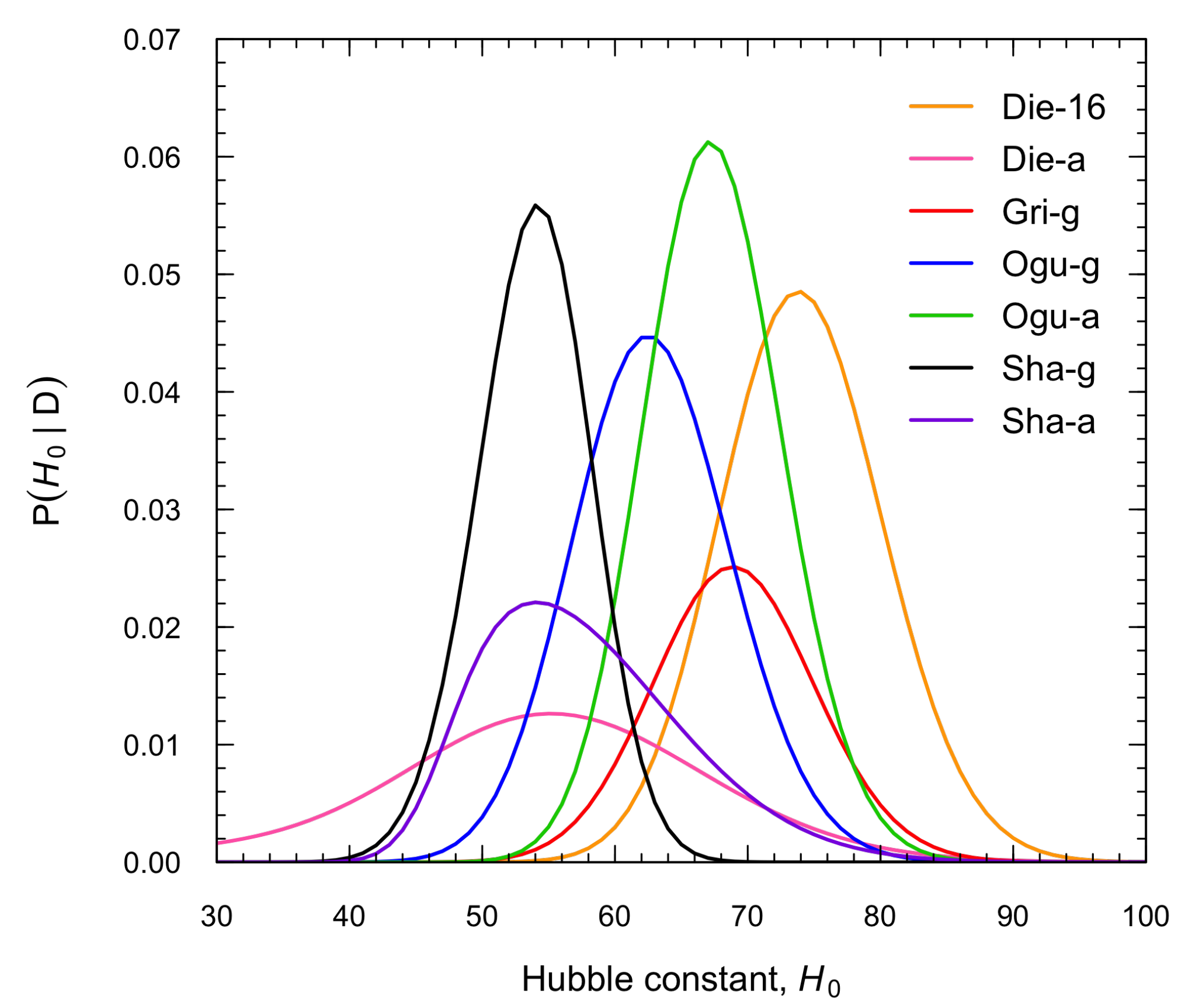
In figure 1 we show the contribution from each model to the total posterior using a flat prior for between and .
Figure 2 summarizes our main result for the posterior and . We have assumed that all model predictions are equal prior validity [but see 27, for a comparison of the performance of the different lensing reconstruction techniques]. The median value and 68% CL for are: for the posterior; and for the posterior. These values of already include a systematic uncertainty at the level which has been added at the end in quadrature to the statistical uncertainty.
V Conclusions
We constrain, for the first time, the Hubble constant following Refsdal’s original idea to use a multiple-lensed SN with measured time delays and precise lens model predictions. By combining the results of multiple lens models, we account for statistical and some systematic errors due to assumptions made during the lens reconstruction. The inferred Hubble constant ranges from for to for . These results are in good agreement with recent constraints from CMB, LSS, and local distance ladders. We use a very weak prior to better show the sensitivity of the Refsdal data to the parameter . Future improved constraints on the observed time delay and magnification will reduce the uncertainty in the Hubble parameter using this technique, and additional estimates derived from different clusters will provide a competitive test for .
References
- [1] Acebron, A., Jullo, E., Limousin, M., et al. 2017, MNRAS, 470, 1809
- [2] Bonvin, V., Courbin, F., Suyu, S. H., et al. 2017, MNRAS, 465, 4914
- [3] Courbin, F., Eigenbrod, A., Vuissoz, C., Meylan, G., & Magain, P. 2005, in IAU Symposium, Vol. 225, Gravitational Lensing Impact on Cosmology, ed. Y. Mellier & G. Meylan, 297–303
- [4] Cover, T. M., & Thomas, J. A. 2006, Elements of Information Theory (Wiley Series in Telecommunications and Signal Processing) (Wiley-Interscience)
- [5] DES Collaboration, Abbott, T. M. C., Abdalla, F. B., et al. 2017, ArXiv e-prints, arXiv:1711.00403
- [6] Diego, J. M., Broadhurst, T., Molnar, S. M., Lam, D., & Lim, J. 2015a, MNRAS, 447, 3130
- [7] Diego, J. M., Broadhurst, T., Zitrin, A., et al. 2015b, MNRAS, 451, 3920
- [8] Diego, J. M., Protopapas, P., Sandvik, H. B., & Tegmark, M. 2005, MNRAS, 360, 477
- [9] Diego, J. M., Tegmark, M., Protopapas, P., & Sandvik, H. B. 2007, MNRAS, 375, 958
- [10] Diego, J. M., Broadhurst, T., Chen, C., et al. 2016, MNRAS, 456, 356
- [11] Ebeling, H., Edge, A. C., & Henry, J. P. 2001, ApJ, 553, 668
- [12] Greene, Z. S., Suyu, S. H., Treu, T., et al. 2013, ApJ, 768, 39
- [13] Jauzac, M., Jullo, E., Eckert, D., et al. 2014, ArXiv e-prints 1406.3011, arXiv:1406.3011
- [14] —. 2015a, MNRAS, 446, 4132
- [15] Jauzac, M., Richard, J., Jullo, E., et al. 2015b, MNRAS, 452, 1437
- [16] Jauzac, M., Richard, J., Limousin, M., et al. 2016, MNRAS, 457, 2029
- [17] Johnson, T. L., & Sharon, K. 2016, ApJ, 832, 82
- [18] Kawamata, R., Oguri, M., Ishigaki, M., Shimasaku, K., & Ouchi, M. 2016, ApJ, 819, 114
- [19] Kelly, P. L., Rodney, S. A., Treu, T., et al. 2015, Science, 347, 1123
- [20] —. 2016a, ApJ Letters, 819, L8
- [21] Kelly, P. L., Brammer, G., Selsing, J., et al. 2016b, ApJ, 831, 205
- [22] Kundić, T., Turner, E. L., Colley, W. N., et al. 1997, ApJ, 482, 75
- [23] Lam, D., Broadhurst, T., Diego, J. M., et al. 2014, ApJ, 797, 98
- [24] Limousin, M., Richard, J., Jullo, E., et al. 2016, A&A, 588, A99
- [25] Mahler, G., Richard, J., Clément, B., et al. 2017, ArXiv e-prints, arXiv:1702.06962
- [26] McCully, C., Keeton, C. R., Wong, K. C., & Zabludoff, A. I. 2017, ApJ, 836, 141
- [27] Meneghetti, M., Natarajan, P., Coe, D., et al. 2016, ArXiv e-prints, arXiv:1606.04548
- [28] Oguri, M. 2015, MNRAS, 449, L86
- [29] Planck Collaboration, Ade, P. A. R., Aghanim, N., et al. 2016, A&A, 594, A13
- [30] Refsdal, S. 1964, MNRAS, 128, 307
- [31] Riess, A. G., Macri, L. M., Hoffmann, S. L., et al. 2016, ApJ, 826, 56
- [32] Rodney, S. A., Strolger, L.-G., Kelly, P. L., et al. 2016, ApJ, 820, 50
- [33] Sereno, M., & Paraficz, D. 2014, MNRAS, 437, 600
- [34] Sharon, K., & Johnson, T. L. 2015, ApJ Letters, 800, L26
- [35] Suyu, S. H., Auger, M. W., Hilbert, S., et al. 2013, ApJ, 766, 70
- [36] Suyu, S. H., Bonvin, V., Courbin, F., et al. 2017, MNRAS, 468, 2590
- [37] Treu, T., Brammer, G., Diego, J. M., et al. 2016, ApJ, 817, 60
- [38] Wilson, M. L., Zabludoff, A. I., Keeton, C. R., et al. 2017, ApJ, 850, 94
- [39] Wong, K. C., Suyu, S. H., Auger, M. W., et al. 2017, MNRAS, 465, 4895
- [40] Zitrin, A., Zheng, W., Broadhurst, T., et al. 2014, ApJ Letters, 793, L12