Hilbert’s ‘monkey saddle’ and other curiosities in
the equilibrium problem of three point particles on a circle for repulsive power law forces

It is easy to convey a sense of the challenge posed by Smale’s 7th problem, and by the quest for optimal Riesz $s$-energy $N$-point configurations in general, when $N$ is large. The empirical number count of relative energy minimizers shows a roughly exponential increase with $N$, see [ErHo97]. In the absence of a deterministic algorithm which in polynomially($N$) many steps finds an optimizing configuration, the method of choice has been (quasi-)random searches (with variations on this theme), yet the likelihood that such a search produces a relative minimizer which is not absolute increases dramatically with $N$.

To rigorously prove, or disprove, the exponential increase with $N$ of the number of relative equilibria when $N$ is large is an interesting open problem. As far as we know, it is not even rigorously known whether exponentially increasing upper or lower bounds on the number of relative equilibria exist.

The overwhelmingly large number of relative minimizers which need to be avoided is not the sole source of difficulties for reaching an optimizer. Even in the small $N$ regime, where it would seem reasonable to expect that it should not be difficult to identify all the relative minimizers of the Riesz $s$-energy function of $N$-particle arrangements³³ 3 We will generally speak of particle arrangements on the unit circle because “degenerate configurations” are not configurations in the proper sense. on $\mathbb{S}^{d}$, at least for small $d=1$ and $d=2$, and determine the optimizer(s) amongst them, it is not necessarily easy to work out the answers. To be sure, the $N=2$ particle problem on $\mathbb{S}^{d}$, $d\in\mathbb{N}$, is trivial:⁴⁴ 4 And, of course, it is meaningless to ask for a minimum Riesz pair energy configuration when $N=1$, since one cannot form a pair with a single particle alone. since the Riesz $s$-energy of a pair of particles decreases monotonically with the distance $r$ between the particles in the pair, the energy of the pair is minimized when the two particles are at their furthest possible distance from each other, which is the antipodal configuration. It is clear that this is also the only relative minimizer (up to rotation) when $N=2$. However, already the optimal $N=3$ Riesz $s$-energy arrangement on $\mathbb{S}^{d}$ is an interesting problem.

Although the absolute Riesz $s$-energy minimizers with three particles have been correctly stated (though without detailing the proof)⁵⁵ 5 Incidentally, there is a slip of pen at the pertinent place in Appendix 1 of [NBK14]: “the only equilibrium arrangements” should read “the only stable equilibrium arrangements.” in Appendix 1 of [NBK14], to the best of our knowledge the complete list of critical Riesz $s$-energy arrangements of $N=3$ particles, and their stability, has not previously been discussed rigorously. In this paper we will supply such a discussion.

By a repulsive power-law force equilibrium on $\mathbb{S}^{d}$ we mean the following.

The proper repulsive power-law force of a point particle at ${\boldsymbol{{p}}}^{\prime}\in\mathbb{R}^{d+1}$ onto a point particle at ${\boldsymbol{{p}}}\in\mathbb{R}^{d+1}$ is defined as the negative ${\boldsymbol{{p}}}$-gradient of the Riesz $s$-energy $R_{s}(\left|{\boldsymbol{{p}}}-{\boldsymbol{{p}}}^{\prime}\right|)$, whenever this gradient is well-defined; if not well-defined, we may still define a pseudo force, see below. The total force on a point particle at ${\boldsymbol{{p}}}\in\mathbb{R}^{d+1}$ is the sum of all these forces exerted on it by the other particles in an $N$-particle system. When restricted to move on $\mathbb{S}^{d}$, $d\in\mathbb{N}$, an arrangement of $N$ point particles is said to be in (proper or pseudo) force equilibrium on $\mathbb{S}^{d}$ if the ${\boldsymbol{{p}}}$-gradient of the total Riesz $s$-energy points radially at each particle’s position ${\boldsymbol{{p}}}$.

Such force equilibria with $N=3$ particles are the same on every $\mathbb{S}^{d}$ (after factoring out rotations). Only their stability properties may depend on $d$.

There are three $s$-independent equilibria, which we call universal, and which are obvious to everyone. There are also two $s$-dependent continuous families of not-so-obvious equilibria, which we call non-universal.

One universal repulsive force equilibrium with $N=3$ particles comes to mind immediately: the equilateral triangular configuration is in proper force equilibrium for all $s\in\mathbb{R}$ due to its symmetry, and because it is not degenerate. We will see that w.r.t. motions on $\mathbb{S}^{1}$, depending on $s$, the equilateral triangular configuration will be any of the following: relatively but not absolutely maximizing, a saddle point, only relatively or also absolutely minimizing.

When $s<-1$ the Riesz $s$-energy gradient force of one point particle onto another one is well-defined also when both particles occupy the same point in space, in which case the mutual forces vanishes. Thus, when $s<-1$, the completely degenerate configuration (i.e. all $N$ particles occupy the same point in space) is in proper force equilibrium, and so is any antipodal arrangement (likewise a degenerate configuration, but not completely) with $1\leq n<N$ particles at the North, and $N-n$ particles at the South Pole (up to rotation). When $N=3$, there is only one antipodal arrangement (up to rotation), say with $n=1$. The completely degenerate configuration is manifestly the absolute energy maximizer, while the antipodal arrangements can be relative or even absolute energy minimizers, or saddle points, depending on $s$.

When $s\geq-1$ the Riesz $s$-energy gradient is not well-defined when two particles occupy the same point, yet when $-1\leq s<0$ the degenerate configurations are still absolutely Riesz $s$-energy maximizing, respectively saddles, and so we refer to them as pseudo force equilibria when $-1\leq s<0$. For $s\geq 0$ these degenerate configurations have $+\infty$ Riesz $s$-energy, so that the notion of them being absolute energy maxima or saddles becomes ambiguous; yet by defining the pseudo force of one particle on top of another as a Cauchy-type principal value, which vanishes, we will count the degenerate configurations (one-point, or antipodal) as non-proper pseudo force equilibria when $s\geq 0$.

The interesting part of the $N=3$ problem is the non-obvious existence of two continuous families of non-universal isosceles repulsive power-law force equilibria whose shapes depend on the Riesz parameter $s$. The isosceles families bifurcate off of a common endpoint — the equilateral configuration — at $s=-4$; one of the families also bifurcates off of the antipodal arrangement, at $s=-2$. The bifurcation at $s=-4$ is analytical, the one at $s=-2$ is not. The isosceles triangular configurations are saddle points w.r.t. motions on $\mathbb{S}^{1}$.

We next state our results precisely, then prove them rigorously.

Suppose $N=3$ point particles in Euclidean $\mathbb{E}^{2}$ are located on a circle of radius 1, $\mathbb{S}^{1}\subset\mathbb{E}^{2}$, forming the corners $\{A,B,C\}$ of a non-degenerate triangle with sides $\{a,b,c\}$ having lengths $\{|a|,|b|,|c|\}$, and strictly positive angles $\{\alpha,\beta,\gamma\}$, cf. Fig.1.

$\hskip 136.5733pt\alpha$

$\hskip 233.3125pt\beta$

$\hskip 176.407pt\gamma$

An arrangement of three point particles on $\mathbb{S}^{1}$ labeled $(A,B,C)$ in counter-clockwise manner is characterized by a point $(\alpha,\beta,\gamma)\in[0,\pi]^{3}\cap\{\alpha+\beta+\gamma=\pi\}$, the “fundamental triangle” in $(\alpha,\beta,\gamma)$ space.

Since a triangular arrangement of point particles on $\mathbb{S}^{1}$ remains invariant under cyclic permutation of the counter-clockwise labelling of the points, each geometrical triangular arrangement of point particles is represented three times in the fundamental triangle, with the exception of the equilateral triangular configuration, represented by the center $(\frac{\pi}{3},\frac{\pi}{3},\frac{\pi}{3})$ of the fundamental triangle.

All interior points of the fundamental triangle represent proper $3$-point configurations (no two point particles occupy the same location). Degenerate configurations with precisely two or all three point particles occupying the same location are represented by the edges, respectively corners of the fundamental triangle. Indeed, by inspecting Fig.1 is is clear that when precisely two point particles are being moved to the same location (say particle $B$ is moved to the location of particle $C$), then $\angle(C,A,B)=\alpha\to 0$. But when $\alpha=0$, then $\beta+\gamma=\pi$ means the arrangement is represented by a point on the edge of the fundamental triangle which sits in the $(\beta,\gamma)$ plane. Of special importance are the antipodal arrangements $(\alpha,\beta,\gamma)=(0,\frac{\pi}{2},\frac{\pi}{2})$ (up to permutation) which are located at the midpoints of the edges of the fundamental triangle, and the completely degenerate triangular configuration (i.e. the one-point arrangement) given by $(\alpha,\beta,\gamma)=(0,0,\pi)$ (up to permutation).

Let $r>0$ stand for any of the side lengths of a proper triangular configuration. We now assign each side a standardized Riesz $s$-energy $V_{s}(r)$ of the pair of point particles located at the two end points, defined by⁶⁶ 6 We remark (see Appendix 3 in [NBK14]) that $s\mapsto V_{s}(r)$ is a continuous, monotonically increasing function for all $r>0$, strictly so if $r\neq 1$, and $V_{s}(1)\equiv 0$ for all $s$.

and average these pair energies over the triangular configuration, written as

here we tacitly used that $|a|=2\sin\alpha$, $|b|=2\sin\beta$, and $|c|=2\sin\gamma$. We define the minimal average standardized Riesz pair-energy of $N=3$ particles on a unit circle as

It is easy to see that the minimal average standardized Riesz pair-energy 5 exists for all $s\in\mathbb{R}$, but the infimum may not be achieved on the set of non-degenerate triangular configurations. We now compactify the space of non-degenerate triangular configurations on the unit circle by adding to it all degenerate three-particle configurations, viz. the linear arrangements in which precisely one of the three angles $\alpha,\beta,\gamma$ is zero, and the single-point arrangement in which two of the three angles $\alpha,\beta,\gamma$ are zero. We also assign an extended real Riesz $s$-energy to a pair with vanishing distance $r=0$ in terms of $\lim_{r\downarrow 0}V_{s}(r)$, viz.

With these stipulations 4 is a lower-semicontinuous function of two of the three angles, say $(\alpha,\beta)\in[0,\pi]^{2}\cap\{\alpha+\beta\leq\pi\}$ (and with $\gamma=\pi-\alpha-\beta$), so a minimizer for 5 always exists. It coincides with the minimizer of the total Riesz $s$-energy as defined in [Schw16], see the introduction.

We will prove the following theorems. The first one lists all the absolute minimizers (see Appendix 1 of [NBK14]).

The next theorem lists all absolute maximizers on $\mathbb{S}^{1}$.

Recalling the usual notion of a relative minimizer / maximizer of (the extended) 4, we define a relative minimizer as any triple $(\alpha_{*},\beta_{*},\gamma_{*})$ of non-negative angles satisfying $\alpha_{*}+\beta_{*}+\gamma_{*}=\pi$ such that $\langle V_{s}\rangle(\alpha_{*},\beta_{*},\gamma_{*})\leq\langle V_{s}\rangle(\alpha,\beta,\gamma)$ for all triples $(\alpha,\beta,\gamma)$ of non-negative angles satisfying $\alpha+\beta+\gamma=\pi$ in a small enough neighborhood of $(\alpha_{*},\beta_{*},\gamma_{*})$, with strict “$<$” holding for some of them; a relative maximizer is defined by replacing “$\leq$” with “$\geq$” and “$<$” by “$>$.”

The next theorem lists all relative minimizers / maximizers on $\mathbb{S}^{1}$ which are not absolute.

The theorems stated above do not depend on the notion of proper force equilibrium, introduced next in terms of $\alpha$ and $\beta$ derivatives of $\langle V_{s}\rangle$. A triple $(\alpha_{*},\beta_{*},\gamma_{*})$ of non-negative angles satisfying $\alpha_{*}+\beta_{*}+\gamma_{*}=\pi$ is called a proper force equilibrium if both $\partial_{\alpha}\langle V_{s}\rangle(\alpha,\beta,\pi-\alpha-\beta)|_{*}=0$ and $\partial_{\beta}\langle V_{s}\rangle(\alpha,\beta,\pi-\alpha-\beta)|_{*}=0$, where “$...|_{*}$” means the expression $...$ to its left is evaluated with $\alpha=\alpha_{*}$ and $\beta=\beta_{*}$, so also $\gamma=\gamma_{*}$. The next theorem lists all proper equilibria under a repulsive power-law force.

As explained in the introduction, a Cauchy principal-value type definition of a pseudo force can be stipulated whenever the proper force is not defined. This vindicates the following.

With the help of this definition it is easy to prove

With the help of the notions of a proper, respectively a non-proper pseudo force equilibrium we are now in the position to define “saddle points.”

The next theorem lists all saddle points of 4.

Lastly, we describe in some detail the non-universal, isosceles, proper force equilibria, stipulating a representation $(\alpha,\beta,\gamma)(s)$ with $\alpha=\beta$.

Our results are illustrated by the following diagram.

We begin with the pseudo force equilibria by proving

The force of one point particle on another is not proper if and only if $s\geq-1$ and both particles occupy the same location. By Definition 1, the pseudo force of any one of these two particles on the other vanishes. Therefore, when $s\geq-1$ we have the following two possibilities:

(i) all three particles occupy the same position — in that case the total pseudo force on any one of them vanishes, so this arrangement is a pseudo force equilibrium;

(ii) only two of the three particles occupy the same position — in that case the total pseudo force on any one of the two particles with coincidental positions is given by the proper force of the remaining third particle on it, while the total force on the third particle is the sum of the proper forces of the two “coincident” particles on it. But then, the only way the total force on each and any one of the three particles can point radial is when the arrangement is antipodal, so the antipodal arrangement is a pseudo force equilibrium, too.

Since these two cases exhaust all possibilities, and since in either case the arrangement is manifestly reflection-symmetric about a diameter of $\mathbb{S}^{1}$, Proposition 1 is proved. $\square$

The proof of Proposition 1 identifies the antipodal and the single-point arrangements as the only possible $N=3$ pseudo force equilibria, and thereby also proves Theorem 5.

We now turn our attention to the proper force equilibria. Proposition 5 has the following counterpart.

The condition for a triple $(\alpha_{*},\beta_{*},\gamma_{*})$ of non-negative angles satisfying $\alpha_{*}+\beta_{*}+\gamma_{*}=\pi$ to be a proper force equilibrium of three particles on $\mathbb{S}^{1}$ consists of the pair of equations $\partial_{\alpha}\langle V_{s}\rangle(\alpha,\beta,\pi-\alpha-\beta)|_{*}=0$ and $\partial_{\beta}\langle V_{s}\rangle(\alpha,\beta,\pi-\alpha-\beta)|_{*}=0$, where “$...|_{*}$” means the expression $...$ to its left is evaluated with $\alpha=\alpha_{*}$ and $\beta=\beta_{*}$, so also $\gamma=\gamma_{*}$. Carrying out the differentiations, and cancelling common factors, yields the pair of equations

This is equivalent to

together with $\alpha_{*}+\beta_{*}+\gamma_{*}=\pi$, which for all $s\in\mathbb{R}$ has the obvious solution $\alpha_{*}=\beta_{*}=\gamma_{*}=\pi/3$, namely the equilateral triangular configuration on $\mathbb{S}^{1}$ (which is reflection-symmetric through even three different diameters of $\mathbb{S}^{1}$).

To show that any other solution of 13 satisfying $\alpha_{*}+\beta_{*}+\gamma_{*}=\pi$ is reflection-symmetric about a diameter of $\mathbb{S}^{1}$, we need to discuss the function $\frac{\cos(\varphi)}{\sin^{s+1}(\varphi)}=:F_{s}(\varphi)$ for $\varphi\in(0,\pi)$, together with its behavior as $\varphi\downarrow 0$ and $\varphi\uparrow\pi$; see Fig.4.

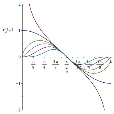
First of all, since $\sin(\varphi)\neq 0$ on the open interval $(0,\pi)$, for each $s\in\mathbb{R}$ the function $F_{s}(\varphi)$ is infinitely often continuously differentiable on $(0,\pi)$, and since $\sin(\varphi)=\sin(\pi-\varphi)$ and $\cos(\varphi)=-\cos(\pi-\varphi)$, we have $F_{s}(\varphi)=-F_{s}(\pi-\varphi)$ on $\varphi\in(0,\pi)$, i.e. $F_{s}(\varphi)$ is reflection-antisymmetric about $\varphi=\pi/2$, where it vanishes. Moreover, $F_{s}(\varphi)>0$ on $(0,\pi/2)$ and, by antisymmetry, $F_{s}(\varphi)<0$ on $(\pi/2,\pi)$. As a consequence, any triple $(\alpha_{*},\beta_{*},\gamma_{*})$ of non-negative angles satisfying 13 and $\alpha_{*}+\beta_{*}+\gamma_{*}=\pi$ must have $F_{s}(\alpha_{*})\geq 0$. For suppose not, i.e. suppose $F_{s}(\alpha_{*})<0$. Then $(\alpha_{*},\beta_{*},\gamma_{*})\in(\pi/2,\pi]^{3}$, which violates the constraint $\alpha_{*}+\beta_{*}+\gamma_{*}=\pi$.

Thus it suffices to discuss $F_{s}$ restricted to the pre-image of $F_{s}\geq 0$. Since the behavior of $F_{s}(\varphi)$ near $\varphi=0$ depends on $s$, we now distinguish the cases $s>-1$, $s=1$, and $s<-1$.

Case $s>-1$. Since $\sin(0)=0=\sin(\pi)$, while $\cos(0)=1=-\cos(\pi)$, when $s>-1$ the function $\varphi\mapsto F_{s}(\varphi)$ is not defined at $\varphi=0$ and not at $\varphi=\pi$, where it diverges to $\pm\infty$, respectively. This already rules out any degenerate configuration (at least one angle $=0$) from being a proper force equilibrium when $s>-1$.

Moreover, it is easy to see that $F_{s}(\varphi)$ is strictly monotonically decreasing on $\varphi\in(0,\pi)$, when $s>-1$. For any $\ell\geq 0$, the equation $F_{s}(\varphi)=\ell$ therefore has only one solution $\varphi_{*}\in(0,\pi)$. But this means that $\alpha_{*}=\beta_{*}=\gamma_{*}$, and now $\alpha_{*}+\beta_{*}+\gamma_{*}=\pi$ forces $\alpha_{*}=\pi/3$.

In geometric terms, when $s>-1$ the equilateral triangular configuration is the only proper force equilibrium of three point particles on $\mathbb{S}^{1}$.

Case $s=-1$. Clearly, $F_{-1}(\varphi)\equiv\cos(\varphi)$, so $F_{-1}(\varphi)$ is well-defined on the closed interval $[0,\pi]$. Yet, since $\cos(\varphi)$ decreases strictly monotonically from $1$ to $-1$ when $\varphi$ varies through $[0,\pi]$, the same conclusion as in the previous case holds: the equilateral triangular configuration is the only proper $s=-1$-force equilibrium of three point particles on $\mathbb{S}^{1}$.

Case $s<-1$. Now $F_{s}(\varphi)$ is well-defined on the closed interval $\varphi\in[0,\pi]$, with $F_{s}(0)=0=F_{s}(\pi)$. Since also $F_{s}(\pi/2)=0$, the level value $\ell=0$ now offers three different possible values for the three angles $\alpha_{*}$, $\beta_{*}$, $\gamma_{*}$ to satisfy 13 with $\alpha_{*}+\beta_{*}+\gamma_{*}=\pi$. Up to permutations, there are exactly two possibilities:

(i) $(\alpha_{*},\beta_{*},\gamma_{*})=(0,0,\pi)$ (the completely degenerate configuration);

(ii) $(\alpha_{*},\beta_{*},\gamma_{*})=(\pi/2,\pi/2,0)$ (the antipodal arrangement).

Next, let $\ell>0$. In this case there is no possible $\varphi_{*}\in[\pi/2,\pi]$ for which $F_{s}(\varphi_{*})=\ell$, and we seek $\varphi_{*}\in(0,\pi/2)$ for which $F_{s}(\varphi_{*})=\ell$. We show that, depending on $\ell$, there can be exactly two, exactly one, or no value of $\varphi_{*}\in(0,\pi/2)$ for which $F_{s}(\varphi_{*})=\ell$.

From the facts that $F_{s}(0)=0=F_{s}(\pi/2)$ when $s<-1$, that $F_{s}(\varphi)>0$ for $\varphi\in(0,\pi/2)$, and that $\varphi\mapsto F_{s}(\varphi)$ is continuous, it follows that $F_{s}(\varphi)$ has a maximum in $(0,\pi/2)$. Clearly, if $\ell$ surpasses this maximum value of $F_{s}(\varphi)$, then there is no $\varphi_{*}$ satisfying $F_{s}(\varphi_{*})=\ell$.

Since $\varphi\mapsto F_{s}(\varphi)$ is differentiable (infinitely often, actually) on $(0,\pi/2)$, any such maximum is taken at a critical point, where $F_{s}^{\prime}(\varphi)=0$. Differentiating $F_{s}$ w.r.t. $\varphi$ and simplifying, we find that the equation $F_{s}^{\prime}(\varphi)=0$ for $\varphi\in(0,\pi/2)$ is equivalent to

which in turn (using $\sin^{2}\varphi+\cos^{2}\varphi=1$) is equivalent to

Since $s<-1$, there is a unique $\phi=\arccos\sqrt{-1/s}\in(0,\pi/2)$ satisfying 15.

Thus, for $s<-1$ there exists in $(0,\pi/2)$ a unique maximum of $F_{s}(\varphi)$, at $\varphi=\phi$, with value $L(s)$ (say). So when $s<-1$, then $F_{s}(\varphi)$ increases monotonically and continuously from $0$ to $L(s)$ when $\varphi$ increases through $[0,\phi]$, and $F_{s}(\varphi)$ decreases monotonically and continuously from $L(s)$ to $0$ when $\varphi$ increases through $[\phi,\pi/2]$.

It follows that if $\ell=L(s)$, then there is a unique value $\varphi_{*}$ satisfying $F_{s}(\varphi_{*})=\ell$, namely $\varphi_{*}=\phi(s)$. If 13 together with $\alpha_{*}+\beta_{*}+\gamma_{*}=\pi$ is satisfied with $\alpha_{*}=\phi(s)$, then all three angles $\alpha_{*}$, $\beta_{*}$, $\gamma_{*}$ must coincide. But this can lead to a proper force equilibrium if and only if $\phi(s)=\pi/3$. Incidentally, by 15 this happens if and only if $1+s/4=0$, or $s=-4$. As already remarked, the equilateral configuration is manifestly reflection-symmetric about a diameter of $\mathbb{S}^{1}$.

Yet if $0<\ell<L(s)$, there are precisely two different values of $\varphi_{*}$, satisfying $0<\varphi_{*}^{(1)}<\varphi_{*}^{(2)}<\pi/2$, for which $F_{s}(\varphi_{*})=\ell$. This now implies that for any possible solution of 13 with value $F_{s}(\alpha_{*})=\ell\in(0,L(s))$, satisfying $\alpha_{*}+\beta_{*}+\gamma_{*}=\pi$, at least two of the three angles $\alpha_{*}$, $\beta_{*}$, $\gamma_{*}$ must coincide, because there are only two possible values, $\varphi_{*}^{(1)},\varphi_{*}^{(2)}$ which any of the three angles $\alpha_{*}$, $\beta_{*}$, $\gamma_{*}$ can take. But then, since for $\ell>0$ none of the angles can be $0$, any possible solution is a proper isosceles triangular configuration with its corners on $\mathbb{S}^{1}$, hence reflection-symmetric about a diameter of $\mathbb{S}^{1}$.

The proof of the proposition is complete. $\square$

Proposition 2, and more so its proof, reveal a number of important facts about the proper force equilibria of three particles on $\mathbb{S}^{1}$, which we summarize as

Furthermore, Propositions 1 and 2, and their proofs, in concert reveal

These corollaries show that Propositions 1 and 2, and their proofs, exhaust the list of force equilibria (proper or pseudo) of $N=3$ particles on $\mathbb{S}^{1}$ when $s\geq-1$: the equilateral configuration (proper), the antipodal arrangement (pseudo), and the single-point arrangement (pseudo). Their proofs have also yielded, as a byproduct, that these three equilibria (proper for $s<-1$) are universal. Since a universal equilibrium is by definition $s$-independent, and since the ones we have identified also exhaust the list of all equilibria for when $s\geq-1$, it follows that our list of universal equilibria is complete.

Propositions 1 and 2 and their proofs do not identify any non-universal equilibria, which by Corollary 2 can at most exist when $s<-1$. This is the content of the next proposition.

We already showed that there are no non-universal equilibria for $s\in[-1,\infty)$, and since pseudo force equilibria by definition cannot exist for $s<-1$, any non-universal equilibrium must be a proper force equilibrium with $s<-1$.

Thanks to Proposition 2, any proper equilibrium for $s<-1$ must correspond to a point on a height of the fundamental triangle. Its three heights meet at the center of the fundamental triangle, and we already know that the center corresponds to the equilateral equilibrium configuration. Moreover we know that the two end points of each height also correspond to equilibra, namely the antipodal arrangement (where a height meets the midpoint of a side) and the completely degenerate configuration (where a height meets a corner). These equilibria are universal. Thus any non-universal equilibrium would have to correspond to a point on the height either between the center and a midpoint of a side, or between the center and a corner, of the fundamental triangle.

Since each height represents the same geometrical situation, we work with the height which corresponds to choosing $\alpha=\beta$, and parametrize the height with $\gamma$. The equilibria are then determined by the critical points $\gamma_{*}$ of the map $\gamma\mapsto\langle V_{s}\rangle\big(\tfrac{\pi-\gamma}{2},\tfrac{\pi-\gamma}{2},\gamma\big)$, the standardized Riesz $s$-energy averaged over the pairs of an isosceles triangle $\big(\frac{\pi-\gamma}{2},\frac{\pi-\gamma}{2},\gamma\big)$ with $\gamma\in[0,\pi]$. For $s<-1$ these agree with the critical points of the map $\gamma\mapsto U_{s}(\gamma)$, given by

Fig.5 shows $U_{s}$ graphed vs. $\gamma$ for a selection of $s$ values. The graphs are monotonically ordered with $s$, decreasing with $s$, which follows from 16.

Even though the figure displays the graphs only for a finite selection of $s$-values, it guides us toward our goal: it shows the $s$-independent critical points $\gamma_{*}\in\{0,\pi/3,\pi\}$ for $s<-1$, and it suggests exactly one additional critical point $\gamma_{*}(s)\in(0,\pi/3)$ when $s\in(-4,-2)$, and exactly one additional critical point $\gamma_{*}(s)\in(\pi/3,\pi/2)$ when $s\in(-\infty,-4)$. Thus guided by Fig.5 we show:

Recall that for $s<-1$ all force equilibria are proper. Hence taking the $\gamma$-derivative of $U_{s}(\gamma)$ (see 16), using $\sin(\tfrac{\pi-\gamma}{2})=\cos(\tfrac{\gamma}{2})$, which yields

we look for zeros of 17 for $\gamma\in(0,\pi/2)$ other than $\gamma_{*}=\pi/3$. Recall that we already showed that all non-degenerate configurations have their angle $\gamma_{*}(s)\in(0,\pi/2)$. Using $\sin(\gamma)=2\sin(\tfrac{\gamma}{2})\cos(\tfrac{\gamma}{2})$ and $\cos(\gamma)=1-2\sin^{2}(\tfrac{\gamma}{2})$, and simplifying, we rewrite 17 as

For $\gamma\in(0,\pi)$, both $\cos(\tfrac{\gamma}{2})>0$ and $\sin(\tfrac{\gamma}{2})>0$, so a zero of $U_{s}^{\prime}(\gamma)$ for $\gamma\in(0,\pi)$ can only come from the factor in square parentheses.

Defining $2\sin(\tfrac{\gamma}{2})=:\xi$ the factor in square parentheses becomes

and we seek its zeros $\xi_{*}$ for $\xi\in(0,\surd{2})$; note that $0<\gamma_{*}(s)<\pi/2$ for $s<-2$ implies that $0<\xi_{*}(s)<\sqrt{2}$ for $s<-2$.

Obviously $\xi_{*}^{(1)}=1$ is one zero of $g_{s}(\xi)$, independently of $s$ — it corresponds to $\gamma=\pi/3$, the equilateral triangular configuration. We now ask whether there are any other zeros of $g_{s}(\xi)$ in $(0,\surd{2})$.

To answer that question we compute $g_{s}^{\prime}(\xi)=|s|\xi^{|s|-1}-2(|s|-2)\xi^{|s|-3}=|s|\xi^{|s|-3}\big(\xi^{2}-2\tfrac{|s|-2}{|s|}\big)$. Clearly, the factor $|s|\xi^{|s|-3}>0$ when $\xi>0$.

Turning first to claim (a), part one, let $-2\leq s<-1$. Then the factor $\big(\xi^{2}-2\tfrac{|s|-2}{|s|}\big)>0$, too. Thus, if $-2\leq s<-1$ then $\xi\mapsto g_{s}(\xi)$ is strictly monotonic increasing on $(0,\surd{2})$, and since $\xi=1$ is a (universal) zero of $g_{s}(\xi)$, there are no other zeros. This establishes the first part of claim (a). On the other hand, let $s=-4$; then, since $g_{-4}(\xi)=\xi^{4}-2\xi^{2}+1=(\xi^{2}-1)^{2}$, once again $\xi_{*}^{(1)}=1$ is the only zero of $g_{s}(\xi)$ in the open interval $(0,\surd{2})$. This establishes the second part of claim (a).

References

- [And83] Andersson, S., Eine Beschreibung komplexer anorganischer Kristallstrukturen, Angew. Chem. 95, 67–80 (1983).
- [AtSu03] Atiyah, M., and Sutcliffe, P., Polyhedra in physics, chemistry, and geometry, Milan J. Math. 71, 33–58 (2003).
- [Bec84] Beck, J., Sums of distances between points on a sphere — an application of the theory of irregularities of distribution to discrete geometry, Mathematica 31, 33–41 (1984).
- [BeHa77] Berman, J., and Hanes, K. Optimizing the Arrangement of Points on the Unit Sphere, Math. Comp. 31, 1006–1008 (1977).
- [BeSa15] Bétermin, L., and Sandier, E., Renormalized Energy and Asymptotic Expansion of Optimal Logarithmic Energy on the Sphere, Constructive Approx. eprint: DOI:10.1007/s00365-016-9357-z (2017).
- [Bjo56] Björck, G., Distributions of positive mass, which maximize a certain generalized energy integral, Ark. Mat. 3, 255–269 (1956).
- [BCM] Bowick, M.J., Cecka, C., and Middleton, A., http://tristis.phy.syr.edu/thomson/thomson.php
- [BHS12] Brauchart, J.S., Hardin, D.P., and Saff, E.B., “The next-order term for optimal Riesz and logarithmic energy asymptotics on the sphere,” pp. 31–61 in Recent advances in orthogonal polynomials, special functions, and their applications (J. Arvesú and G. López Lagomasino, eds.), Contemporary Mathematics, 578, AMS, Providence, RI (2012).
- [CoKu07] Cohn, H., and Kumar, A., “Universally optimal distribution of points on spheres,” J. Amer. Math. Soc. 20:1, 99–148 (2007).
- [DLT02] Dragnev, P.D., Legg, D.A., and Townsend, D.W., “Discrete logarithmic energy on the sphere,” Pacific J. Math. 207:2, 345–358 (2002).
- [ErHo97] Erber, T., and Hockney, G.M., “Complex systems: equilibrium configurations of equal charges on a sphere ,” pp. 495-594 in Adv. Chem. Phys. XCVIII (I. Prigogine, S. A. Rice, Eds.), Wiley, New York (1997).
- [Fek23] Fekete, M., “Über die Verteilung der Wurzeln bei gewissen algebraischen Gleichungen mit ganzzahligen Koeffizienten,” Math. Z. 17, 228–249 (1923).
- [FejT56] Fejes Tóth, L., On the sum of distances determined by a point set, Acta. Math. Acad. Sci. Hungar. 7, 397–401 (1956).
- [HaSa04] Hardin, D.P., and Saff, E.B., Discretizing manifolds via minimum energy points, Notices of the AMS 51, 1186–1194 (2004).
- [HiCV52] Hilbert, D., and Cohn-Vossen, S., “Geometry and the Imagination” (2nd ed.), Chelsea, N.Y. (1952).
- [HoSh11] Hou, X., and Shao, J., “Spherical distribution of 5 points with maximal distance sum,” Discrete Comput. Geom. 46:1, 156–174 (2011).
- [MKS77] Melnyk, T.W., Knop, O., and Smith, W.R., “Extremal arrangements of points and unit charges on a sphere: equilibrium configurations revisited,” Canad. J. Chem. 55:10, 1745–1761 (1977).
- [NBK14] Nerattini, R., Brauchart, J.S., and Kiessling, M.K.-H., Optimal -point configurations on the sphere: “Magic” numbers and Smale’s 7th problem, J. Stat. Phys. 157:1138–1206 (2014).
- [RSZ94] Rakhmanov, E.A., Saff, E.B., and Zhou, Y.M., Minimal discrete energy on the sphere, Math. Res. Lett. 1, 647–662 (1994).
- [RSZ95] Rakhmanov, E.A., Saff, E.B., and Zhou, Y.M., “Electrons on the sphere,” pp. 111–127 in Computational Methods and Function Theory (R. M. Ali, S. Ruscheweyh, and E. B. Saff, eds.), World Scientific (1995).
- [SaKu97] Saff, E.B., and Kuijlaars, A.B.J., Distributing many points on a sphere, Math. Intelligencer 19, 5–11 (1997).
- [Sat80] Sattinger, D.H. Bifurcation and Symmetry Breaking in Applied Mathematics, Bull. Amer. Math. Soc. 3 779–819 (1980).
- [Schw16] Schwartz, R.E., The Phase Transition in 5 Point Energy Minimization, (eprint) arXiv:1610.03303v3 [math.OC]
- [Sma98] Smale, S. Mathematical problems for the next century, Math. Intelligencer 20, 7–15 (1998); see also version 2 on Steve Smale’s home page: http://math.berkeley.edu/smale/.
- [Sto75] Stolarsky, K.B., Spherical distributions of points with maximal distance sums are well spaced, Proc. Amer. Math. Soc. 48, 203–206 (1975).
- [Sze24] Szegő, G., Bemerkungen zu einer Arbeit von Herrn M. Fekete: Über die Verteilung der Wurzeln bei gewissen algebraischen Gleichungen mit ganzzahligen Koeffizienten, Math. Z. 21, 203–208 (1924).
- [Tho04] Thomson, J.J., On the structure of the atom: an investigation of the stability and periods of oscillation of a number of corpuscles arranged at equal intervals around the circumference of a circle; with application of the results to the theory of atomic structure, Philos. Mag. 7, 237–265 (1904).
- [Why52] Whyte, L.L., Unique arrangements of points on a sphere, Amer. Math. Monthly 59, 606–611 (1952).
- [Wom09]
Womersley, R.S.,
Robert Womersley’s home page:
http://web.maths.unsw.edu.au/rsw/.