The Sound and the Fury:
Hiding Communications in Noisy Wireless Networks with Interference Uncertainty

Zhihong Liu¹, Jiajia Liu¹²⁵, Yong Zeng¹, Li Yang³, and Jianfeng Ma¹ Affiliation: ¹School of Cyber Engineering, Xidian University, Xi’an, China Affiliation: ²State Key Laboratory of Integrated Service Networks, Xidian University, Xi’an, China Affiliation: Affiliation: ³School of Computer Science and Technology, Xidian University, Xi’an, China Affiliation: ⁵E-mail: liujiajia@xidian.edu.cn

Abstract

Covert communication can prevent the adversary from knowing that a wireless transmission has occurred. In the additive white Gaussian noise channels, a square root law is obtained and the result shows that Alice can reliably and covertly transmit $\mathcal{O}(\sqrt{n})$ bits to Bob in $n$ channel uses. If additional “friendly” node near the adversary can inject artificial noise to aid Alice in hiding her transmission attempt, covert throughput can be improved, i.e., Alice can covertly transmit $\mathcal{O}(\min\{n,\lambda^{\alpha/2}\sqrt{n}\})$ bits to Bob over $n$ uses of the channel ( $\lambda$ is the density of friendly nodes and $\alpha$ is the path loss exponent of wireless channels). In this paper, we consider the covert communication in a noisy wireless network, where Bob and the adversary Willie not only experience the background noise, but also the aggregated interference from other transmitters. Our results show that uncertainty in interference experienced by Willie is beneficial to Alice. When the distance between Alice and Willie $d_{a,w}=\omega(n^{\delta/4})$ ( $\delta=2/\alpha$ is stability exponent), Alice can reliably and covertly transmit $\mathcal{O}(\log_{2}\sqrt{n})$ bits to Bob in $n$ channel uses. Although the covert throughput is lower than the square root law and the friendly jamming scheme, the spatial throughput is higher. From the network perspective, the communications are hidden in “the sound and the fury” of noisy wireless networks, and what Willie sees is merely a “shadow” wireless network. He knows for certain that some nodes are transmitting, but he cannot catch anyone red-handed.

Index Terms:

Physical-layer Security; Covert Communication; Stochastic Geometry; Interference.

I Introduction

Traditional cryptography methods for network security can not solve all security problems. In wireless networks, if a user wishes to communicate covertly without being detected by other detectors, encryption to preventing eavesdropping is not enough [1]. Even if a message is encrypted, the metadata, such as network traffic pattern, can reveal some sensitive information [2]. Furthermore, if the adversary cannot detect the transmission, he has no chance to launch the “eavesdropping and decoding” attack even if he has boundless computing and storage capabilities. On other occasions, such as in a battlefield, soldiers hope to hide their tracks and communicate covertly. Another occasion, such as defeating “Panda-Hunter” attack [3], also needs to prevent the adversary from detecting the transmission behavior of users to protect the location privacy.

Consider the scenario where a transmitter Alice would like to communicate with a receiver Bob covertly over a wireless channel in order to not being detected by a warden Willie. In [4], Bash et al. found a square root law in additive white Gaussian noise (AWGN) channels, that is, Alice can transmit $\mathcal{O}(\sqrt{n})$ bits reliably and covertly to Bob over $n$ uses of wireless channels. The square root law implies pessimistically that the asymptotic privacy rate approaches zero. If Willie does not know the time of the transmission attempts of Alice, Alice can reliably transmit $\mathcal{O}(\min\{(n\log T(n))^{1/2},n\})$ bits to Bob while keeping the Willie’s detector ineffective with a slotted AWGN channel model containing $T(n)$ slots [5]. To improve the performance of covert communication, Lee et al. [6] found that, Willie has measurement uncertainty about its noise level due to the existence of SNR wall [7], then they obtained an asymptotic privacy rate which approaches a non-zero constant. Following Lee’s work, He et al. [8] defined new metrics to gauge the covertness of communication. They took the distribution of noise measurement uncertainty into consideration. Wang et al. [9] considered the covert communication over the discrete memoryless channels (DMC), and found that the privacy rate scales like the square root of the blocklength. Bloch et al. [10] discussed the covert communication problem from a resolvability perspective. He developed an alternative coding scheme such that, if the warden’s channel statistics are known, on the order of $\sqrt{n}$ reliable covert bits may be transmitted to Bob over $n$ channel uses with only on the order of $\sqrt{n}$ bits of secret key. Soltani et al. [11] studied the covert communications on renewal packet channels. They introduced some information-theoretic limits for covert communication over packet channels where the packet timings of legitimate users are governed by a Poisson point process.

Although the research on covert wireless communication focuses on the transmission capability, it is quite different from the works that measure the performance of wireless networks [12][13]. In general, the covertness of communication is due to the existence of noise that the adversary cannot accurately distinguish between the signal and noise. If we can increase the measurement uncertainty of the adversary, the performance of covert communication can be improved. Take the following occasion as an example,

“One day morning you walked in the woods. A lark with beautiful tail feathers was singing. You closed your eyes, listening …Although a little breeze was rustling and tumbling in the woods, you could still hear the sweet lark sing in the clear air of the day. All of a sudden, a crowd of larks flew here, you was drowned in the noisy twitters …You no longer knew whether the lark with beautiful tail feathers was still singing or not …”

Now the lark’s song is submerged in the interference and is difficult to be detected. Interference or jamming is usually considered harmful to wireless communications, but it is also a useful security tool. Cooperative jamming is regarded as a prevalent physical-layer security approach [14][15] in wireless communication environment. Jammers inject additional interferences when the transmitter sends messages in order to interfere the potential eavesdroppers [16][17][18][19]. Sobers et al. [20][21] employed cooperative jamming to obtain covert communication. To achieve the transmission of $\mathcal{O}(n)$ bits covertly to Bob over $n$ uses of the channel, they added a “jammer” to the environment to help Alice for security objectives. Soltani et al. [22][23] considered a network scenario where there are multiple “friendly” nodes that can generate interference to hide the transmission from multiple adversaries. They assumed that the friendly nodes are in collusion with Alice and can determine the closest node to each warden.

Refer to caption — Fig. 1: System configuration of covert wireless communication. Alice wishes to transmit reliably and covertly to Bob. The interferers, or other transmitters (represented by black circles) are distributed according to a two-dimensional PPP in the presence of warden Willie (represented by red cross).

In this work, we consider a large-scale wireless network, where the locations of potential transmitters form a stationary Poisson point process (PPP), and their transmission decisions are made independently (as depicted in Fig. 1). In this scenario, Bob and Willie not only experience noise, but also interference signal from other transmitters simultaneously. Since the measure uncertainty of aggregated interference is greater than the background noise, the uncertainty of Willie will increase along with the increase of interference. Although the other transmitters do not collaborate with Alice, and Bob’s noise increases as well (multiuser interference cancellation technique [24] is not used), we find that the covert communication between Alice and Bob is still possible. Alice can reliably and covertly transmit $\mathcal{O}(\log_{2}\sqrt{n})$ bits to Bob in $n$ channel uses when the distance between Alice and Willie $d_{a,w}=\omega(n^{\delta/2})$ ( $\delta=2/\alpha$ is the stability exponent). Although the covert throughput is lower than the square root law and the friendly jamming scheme, its spatial throughput is higher, and Alice does not presuppose the location knowledge of Willie. From the perspective of network, all transmitters in the network can achieve the same covert throughput with the same transmit power, and the larger transmit power level does not increase the probability of being detected since Willie will also experience a stronger interference. Willie cannot determine which node is transmitting except he can approach very close to a certain node (in this occasion the node will find Willie and stop transmitting). “The sound and the fury” of the noisy wireless channels make the network a “shadow” network to Willie.

Contributions. This paper makes the following contributions:

1.

We considered covert wireless communications in a network scenario, and established the bound on reliable covert bits that may be transmitted. We found that the random interference in a large-scale wireless network makes the network a “shadow network” to Willie, and can achieve a high spatial throughput.
2.

Leveraging on analysis and simulation results, we proposed practical methods to improve the performance of covert communications in noisy wireless networks.

The rest of the paper is structured as follows. We formulate the problem and system model in Section II. Next, we study the covert communication with interference uncertainty in Section III. We then present the discussions in Section IV and conclude our work in Section V.

II Problem Formulation and System Model

In this section, prior to presenting the system model, we give a running example to illustrate the problem of covert wireless communications discussed in this paper.

II-A Motivating Scenario

Covert communication has a very long history. It is always related with steganography [25] which conceals messages in audio, visual or textual content. However, steganography is an application layer communication technique and is not suitable in physical-layer covert communication. The well-known physical-layer covert communication is spread spectrum which is using to protect wireless communication from jamming and eavesdropping [26]. Another kind of covert communications is network covert channels [27][28] in computer networks. While steganography requires some form of content as cover, the network covert channels require network protocols as carrier. In this paper, we consider physical-layer covert communication that employs the background noise and the aggregated interference in wireless channels to hide transmission attempts.

Let us take the source location privacy protection in the Panda-Hunter game [3] as an example. In the Panda-Hunter Game, a sensor network with a large number of sensors has been deployed to monitor the habitat of pandas. As soon as a panda is observed by a sensor, this sensor will store the observation data, and then report the observations to a sink via multi-hop wireless channels. However, there is a hunter (the adversary Willie) in the network who tries to capture the panda. The hunter does not care the readings of sensors, what he really cares is the location of the message originator. To find the message originator near the panda, he listens to a sensor in his vicinity to determine whether this sensor is transmitting message. If he finds a transmitter, he then searches for the next sensor who is communicating with this transmitter. Via this method, he can trace back the routing path until he reaches the message originator and catches the panda. As a result, the source location information becomes critical and must be protected in this occasion.

To tackle this problem, Kamat et al. proposed phantom routing techniques to provide source-location privacy from the perspective of network routing [3]. Phantom routing techniques achieve location privacy by combining flooding and single-path routing together. From another point of view, the physical-layer covert communication can provide another kind of solution to the Panda-Hunter game. If we can hide the transmission from the hunter in noise and interference of the noisy wireless channels, the hunter will not able to determine which sensor is transmitting, and therefore cannot trace back to the source. What the hunter sees is a noisy and a shadow wireless network.

II-B Channel Model

Consider a wireless communication scene where Alice (A) wishes to transmit a message to the receiver Bob (B). Right next to them, a warden Willie (W) is eavesdropping over the wireless channel and trying to find whether or not Alice is transmitting.

We adopt the wireless channel model similar to [4][23], and throughout this paper we use the similar notations. We consider a time-slotted system where the time is divided into successive slots with equal duration. All wireless channels are assumed to suffer from discrete-time AWGN with real-valued symbols. Alice transmits $n$ real-valued symbols $s_{1}^{(a)},s_{2}^{(a)},...,s_{n}^{(a)}$ . The receiver Bob observes the vector $y^{(b)}_{1},y^{(b)}_{2},...,y^{(b)}_{n}$ , where $y^{(b)}_{i}=s_{i}^{(a)}+z^{(b)}_{i}$ , and $z^{(b)}_{i}$ is the noise Bob experiences which can be expressed as $z^{(b)}_{i}=z^{(b)}_{i,0}+I^{(b)}_{i}$ , where $\{z^{(b)}_{i,0}\}_{i=1}^{n}$ are independent and identically distributed (i.i.d.) random variables (RVs) representing the background noise of Bob with $z^{(b)}_{i,0}\sim\mathcal{N}(0,\sigma^{2}_{b,0})$ , and $\{I^{(b)}_{i}\}^{n}_{i=1}$ are i.i.d. RVs characterizing the aggregated interference from other transmitters in the wireless network.

As to Willie, he observes the vector $y^{(w)}_{1},y^{(w)}_{2},...,y^{(w)}_{n}$ , where $y^{(w)}_{i}=s_{i}^{(a)}+z^{(w)}_{i}$ , and $z^{(w)}_{i}$ is the noise Willie experiences which can be expressed as $z^{(w)}_{i}=z^{(w)}_{i,0}+I^{(w)}_{i}$ , where $\{z^{(w)}_{i,0}\}_{i=1}^{n}$ are i.i.d. RVs representing the background noise of Willie with $z^{(w)}_{i,0}\sim\mathcal{N}(0,\sigma^{2}_{w,0})$ , and $\{I^{(w)}_{i}\}^{n}_{i=1}$ are i.i.d. RVs characterizing the aggregated interference Willie experiences.

Suppose each node in the network is equipped with one antenna, and Bob and Willie experience the same background noise power, i.e., $\sigma^{2}_{b,0}=\sigma^{2}_{w,0}$ . Besides, different from the occasion discussed in [23], no location information of Willie and other transmitters is available in our model.

II-C Network Model

Consider a large-scale wireless network, where the locations of transmitters form a stationary Poisson point process (PPP)[29] $\Pi=\{X_{i}\}$ on the plane $\mathbb{R}^{2}$ . The density of the PPP is represented by $\lambda$ , denoting the average number of transmitters per unit area. Suppose each potential transmitter has an associated receiver, the transmission decisions are made independently across transmitters and independent of their locations for each transmitter, and the transmission power employed for each node are constant power $P_{t}$ . Any other channel models with power control or threshold scheduling will have similar results with some scale factors. Suppose the wireless channel is modeled by large-scale fading with path loss exponent $\alpha$ ( $\alpha>2$ ). Let the Euclidean distance between node $i$ and node $j$ is denoted as $d_{i,j}$ . For simplicity, let the channel gain $\mathbf{h}_{i,j}$ of channel between $i$ and $j$ is static over the signaling period, and all links experience unit mean Rayleigh fading. Then, the aggregated interference seen by Bob and Willie are the functional of the underlying PPP $\Pi=\{X_{i}\}$ and the channel gain,

	$\displaystyle I_{i}^{(b)}$	$\displaystyle\equiv$	$\displaystyle\sum_{k\in\Pi}\sqrt{\frac{P_{t}}{d_{b,k}^{\alpha}}}\mathbf{h}_{b,k}\cdot s_{i}^{(k)}\sim\mathcal{N}(0,\sigma^{2}_{I_{b}})$		(1)
	$\displaystyle I_{i}^{(w)}$	$\displaystyle\equiv$	$\displaystyle\sum_{k\in\Pi}\sqrt{\frac{P_{t}}{d_{w,k}^{\alpha}}}\mathbf{h}_{w,k}\cdot s_{i}^{(k)}\sim\mathcal{N}(0,\sigma^{2}_{I_{w}})$		(2)

where each $s_{i}^{(k)}$ is a Gaussian random variable $\mathcal{N}(0,1)$ which represents the signal of the $k$ -th transmitter in $i$ -th channel use, and

	$\displaystyle\sigma^{2}_{I_{b}}$	$\displaystyle=$	$\displaystyle\sum_{k\in\Pi}\frac{P_{t}}{d_{b,k}^{\alpha}}\|\mathbf{h}_{b,k}\|^{2}=\sum_{k\in\Pi}\frac{P_{t}}{d_{b,k}^{\alpha}}\Psi_{b,k},$		(3)
	$\displaystyle\sigma^{2}_{I_{w}}$	$\displaystyle=$	$\displaystyle\sum_{k\in\Pi}\frac{P_{t}}{d_{w,k}^{\alpha}}\|\mathbf{h}_{w,k}\|^{2}=\sum_{k\in\Pi}\frac{P_{t}}{d_{w,k}^{\alpha}}\Psi_{w,k}$		(4)

are shot noise (SN) process, representing the powers of the interference that Bob and Willie experience, respectively. The Rayleigh fading assumption implies $\Psi_{i,j}=|\mathbf{h}_{i,j}|^{2}$ is exponentially distributed with $\mathbb{E}[\Psi_{i,j}]=1$ .

The powers of aggregated interferences, $\sigma^{2}_{I_{w}}$ and $\sigma^{2}_{I_{b}}$ , are RVs which are determined by the randomness of the underlying PPP of transmitters and the fading of wireless channels. Therefore they are difficult to be predicted. Besides, the closed-form distribution of the interference is hard to obtain and we have to bound it.

II-D Hypothesis Testing

To find whether Alice is transmitting or not, Willie has to distinguish between the following two hypotheses,

	$\displaystyle\mathbf{H_{0}}$	$\displaystyle:$	$\displaystyle y_{i}^{(w)}=I_{i}^{(w)}+z_{i,0}^{(w)}$		(5)
	$\displaystyle\mathbf{H_{1}}$	$\displaystyle:$	$\displaystyle y_{i}^{(w)}=\sqrt{\frac{P_{t}}{d_{a,w}^{\alpha}}}\mathbf{h}_{a,w}\cdot s_{i}+I_{i}^{(w)}+z_{i,0}^{(w)}$		(6)

Based on the received vector $\mathbf{y}=(y_{1}^{(w)},...,y_{n}^{(w)})$ , Willie should make a decision on whether the received signal is noise+interference or signal plus noise+interference. We assume that Willie employs a radiometer as his detector, and does the following statistic test

T(\mathbf{y})=\frac{1}{n}\mathbf{y}^{H}\mathbf{y}=\frac{1}{n}\sum^{n}_{k=1}y_{k}^{(w)}*y_{k}^{(w)}>\gamma

(7)

where $\gamma$ denotes Willie’s detection threshold and $n$ is the number of samples.

Let $D_{0}$ and $D_{1}$ be the events that the received signal of Willie is noise+interference and Alice’s signal plus noise+interference, respectively, then the probability of false alarm and missed detection can be denoted as $\mathbb{P}_{FA}=\mathbb{P}\{D_{1}|\mathbf{H_{0}}\}$ and $\mathbb{P}_{MD}=\mathbb{P}\{D_{0}|\mathbf{H_{1}}\}$ , respectively. Willie wishes to minimize his probability of error $\mathbb{P}_{e}^{(w)}=(\mathbb{P}_{FA}+\mathbb{P}_{MD})/2$ , but Alice’s ultimate objective is to guarantee that the average probability of error $\mathbf{E}[\mathbb{P}_{e}^{(w)}]=\mathbf{E}[\mathbb{P}_{FA}+\mathbb{P}_{MD}]/2>1/2-\epsilon$ for an arbitrarily small positive $\epsilon$ .

First of all, Willie has to estimate the power level of noise+interference. The noise $z^{(w)}_{i,0}$ not only comes from the thermal noise in his receiver but also the environmental noise from his surroundings. Besides, the aggregated interference $I_{i}^{(w)}$ he sees is a random variable which is determined by the randomness of the underlying PPP of transmitters and the channel gains. The only way for Willie to estimate the noise+interference level is to gather samples. However, he cannot determine definitely whether the samples he collected contain Alice’s transmission signal or not.

Besides, Alice should guarantee that the transmission is reliable, i.e., the desired receiver (Bob) can decode her message with arbitrarily low average probability of error $\mathbb{P}^{(b)}_{e}$ at long block lengths. For any $\epsilon>0$ , Bob can achieve $\mathbb{P}^{(b)}_{e}<\epsilon$ as $n\rightarrow\infty$ .

In this paper, we use standard Big- $\mathcal{O}$ , Little- $\omega$ , and Big- $\Theta$ notations to describe bounds on asymptotic growth rates. The parameters and notation used in this paper are illustrated in Table I.

TABLE I: parameters and notation

\mathbf{Symbol}

\mathbf{Meaning}

P_{t}

Transmit power

n

Number of channel use

\alpha

Path loss exponent

\delta=2/\alpha

Stability exponent

\Pi=\{X_{i}\}

PPP of potential transmitters

\lambda

Intensity of PPP

\Pi

s_{i}^{(a)}

Alice’s signal in

i

-th channel use

s_{i}^{(k)}

Signal of node

k\in\Pi

i

-th channel use

z_{i,0}^{(b)},~z_{i,0}^{(w)}

(Bob’s, Willie’s) background noise in

i

-th channel use

\sigma_{b,0}^{2},~\sigma_{w,0}^{2}

Power of noise (Bob, Willie) observes

I_{i}^{(b)},~I_{i}^{(w)}

Interference (Bob, Willie) observes in

i

-th channel use

\sigma_{I_{b}}^{2},~\sigma_{I_{w}}^{2}

Power of interference (Bob, Willie) observes

\sigma_{b}^{2},~\sigma_{w}^{2}

Power of noise plus interference (Bob, Willie) observes

d_{i,j}

Distance between

i

and

j

\mathbf{h}_{i,j}

Channel gain of channel between

i

and

j

\Psi_{i,j}

\Psi_{i,j}=|\mathbf{h}_{i,j}|^{2}

is exponentially distributed with

\mathbf{E}[\Psi_{i,j}]=1

\mathcal{N}(\mu,\sigma^{2})

Gaussian distribution with mean

\mu

and variance

\sigma^{2}

\mathbb{P}_{FA}

Probability of false alarm

\mathbb{P}_{MD}

Probability of missed detection

\mathbf{E}[X]

Mean of random variable

X

\mathbf{Var}[X]

Variance of random variable

X

q(\lambda)

Outage probability for a typical receiver

\tau(\lambda)

Spatial throughput of successful transmissions

III Covert Communication With Interference Uncertainty in Noisy Wireless Networks

In this section, we first present a theorem on the amount of information that can be transmitted covertly and reliably over AWGN channels in a noisy wireless network, then present its achievability and converse proof.

Theorem 1. Suppose a large-scale wireless network, where transmission decisions of nodes are made randomly, and the locations of transmitters form a PPP on the plane $\mathbb{R}^{2}$ . When the distance between Alice and Willie $d_{a,w}=\omega(n^{\delta/4})$ , Alice can covertly and reliably transmit $\mathcal{O}(\log_{2}\sqrt{n})$ bits to Bob in $n$ channel uses in the case that $\alpha=4$ ( $\delta=2/\alpha$ is the stability exponent). Conversely, if the distance $d_{a,w}=\mathcal{O}(n^{\delta/4})$ , and Alice attempts to send $\omega(\log_{2}\sqrt{n})$ bits to Bob in $n$ channel uses, then, as $n\rightarrow\infty$ , either Willie can detect her transmission with arbitrarily low probability of error $\mathbb{P}^{(w)}_{e}$ , or Bob cannot decode Alice’s message with arbitrarily low error probability $\mathbb{P}^{(b)}_{e}$ .

III-A Achievability

To transmit messages to Bob reliably, Alice should encode her messages. In this paper, we use the classical encoder scheme used in [4] and suppose that Alice and Bob have a shared secret of sufficient length. At first, Alice and Bob leverage the shared secret and random coding arguments to generate a secret codebook. Then Alice’s channel encoder takes as input message of length $L$ bits and encodes them into codewords of length $n$ at the rate of $R=L/n$ bits/symbol. Each codeword is a zero-mean Gaussian random $\mathcal{N}(0,P_{t})$ where $P_{t}$ is the transmit power.

III-A1 Covertness

Alice’s objective is to hide her transmission attempts from being detected by Willie. If Willie’s probability of error $\mathbf{E}[\mathbb{P}_{e}^{(w)}]=\mathbf{E}[\mathbb{P}_{FA}+\mathbb{P}_{MD}]/2>1/2-\epsilon$ for an arbitrarily small positive $\epsilon$ , then we can say that the covertness is satisfied.

Different from the cases studied in [4][23], Alice and Bob are located in a noisy wireless network. No location information of Willie and other potential transmitters is available, and Alice cannot collude with other “friendly” nodes. Willie not only experiences the background noise, but also the aggregated interference from other transmitters in the network. Therefore the power of noise and interference Willie experiences can be expressed as

\sigma_{w}^{2}=\sigma^{2}_{w,0}+\sigma_{I_{w}}^{2},

(8)

where $\sigma^{2}_{w,0}$ is the power of the background noise, $\sigma_{I_{w}}^{2}$ is the power of the aggregated interference from other transmitters (defined in Equ. (4)). In general, the interference is more difficult to be predicted than the background noise, since the randomness of aggregated interference comes from the randomness of PPP $\Pi$ and the fading channels, especially in a mobile wireless network.

Let $\mathbb{P}_{0}$ be the joint probability density function (PDF) of $\mathbf{y}=(y_{1}^{(w)},...,y_{n}^{(w)})$ when $\mathbf{H_{0}}$ is true, $\mathbb{P}_{1}$ be the joint PDF of $\mathbf{y}$ when $\mathbf{H_{1}}$ is true. Using the same analysis methods and the results from [4][23], if Willie employs the optimal hypothesis test to minimize his probability of detection error $\mathbb{P}_{e}^{(w)}$ , then

\mathbb{P}_{e}^{(w)}\geq\frac{1}{2}-\sqrt{\frac{1}{8}D(\mathbb{P}_{1}||\mathbb{P}_{0})},

(9)

where $D(\mathbb{P}_{1}||\mathbb{P}_{0})$ is the relative entropy between $\mathbb{P}_{1}$ and $\mathbb{P}_{0}$ , and the lower bound $\mathbb{P}_{e}^{(w)}$ can be expressed as follows

$\displaystyle\mathbb{P}_{e}^{(w)}$	$\displaystyle\geq$	$\displaystyle\frac{1}{2}-\sqrt{\frac{n}{8}}\cdot\frac{P_{t}\Psi_{a,w}}{2\sigma_{w}^{2}d^{\alpha}_{a,w}}$	(10)
	$\displaystyle=$	$\displaystyle\frac{1}{2}-\sqrt{\frac{n}{8}}\cdot\frac{P_{t}\Psi_{a,w}}{2d^{\alpha}_{a,w}}\cdot\frac{1}{\sigma^{2}_{w,0}+\sigma_{I_{w}}^{2}}$
	$\displaystyle\geq$	$\displaystyle\frac{1}{2}-\sqrt{\frac{n}{8}}\cdot\frac{P_{t}\Psi_{a,w}}{2d^{\alpha}_{a,w}}\cdot\frac{1}{\sigma_{I_{w}}^{2}}.$

The last step is due to $\sigma^{2}_{w,0}<<\sigma_{I_{w}}^{2}$ , since in a dense and large-scale wireless network, the background noise is negligible compared to the aggregated interference from other transmitters [30]. Then the mean of $\mathbb{P}_{e}^{(w)}$ is

	$\displaystyle\mathbf{E}[\mathbb{P}_{e}^{(w)}]$	$\displaystyle\geq$	$\displaystyle\frac{1}{2}-\sqrt{\frac{n}{8}}\cdot\frac{P_{t}\mathbf{E}[\Psi_{a,w}]}{2d^{\alpha}_{a,w}}\cdot\mathbf{E}\biggl[\frac{1}{\sigma_{I_{w}}^{2}}\biggr]$		(11)
		$\displaystyle=$	$\displaystyle\frac{1}{2}-\sqrt{\frac{n}{8}}\cdot\frac{P_{t}}{2d^{\alpha}_{a,w}}\cdot\mathbf{E}\biggl[\frac{1}{\sigma_{I_{w}}^{2}}\biggr]$		(11)

for all links experience unit mean Rayleigh fading.

To estimate $\mathbf{E}[1/\sigma_{I_{w}}^{2}]$ , we should have the closed-form expression of the distribution of $\sigma^{2}_{I_{w}}=\sum_{k\in\Pi}\frac{P_{t}}{d_{w,k}^{\alpha}}\Psi_{w,k}$ . However, $\sigma^{2}_{I_{w}}$ is an RV whose randomness originates from the random positions in PPP $\Pi$ and the fading channels. It obeys a stable distribution without closed-form expression for its PDF or cumulative distribution function (CDF). To address wireless network capacity, Weber et al. [31] employed tools from stochastic geometry to obtain asymptotically tight bounds on the distribution of the signal-to-interference (SIR) level in a wireless network, yielding tight bounds on its complementary cumulative distribution function (CCDF). Next we leverage the bounds on CCDF to estimate the expectation $\mathbf{E}[1/\sigma_{I_{w}}^{2}]$ .

Define a random variable

\mathbf{Y}=\frac{\Sigma_{i\in\Pi}P_{t}\Psi_{i,w}d^{-\alpha}_{i,w}}{P_{t}\Psi_{a,w}d^{-\alpha}_{a,w}}=\frac{\sigma^{2}_{I_{w}}}{P_{t}\Psi_{a,w}d^{-\alpha}_{a,w}},

(12)

then, the lower bound on the CCDF of RV $\mathbf{Y}$ , $\bar{F}^{l}_{\mathbf{Y}}(y)$ , can be expressed as [31],

\bar{F}_{\mathbf{Y}}^{l}(y)=\kappa\lambda y^{-\delta}+\mathcal{O}(y^{-2\delta}),

(13)

where $\kappa=\pi\mathbf{E}[\Psi^{\delta}]\mathbf{E}[\Psi^{-\delta}]\mathbf{E}[d^{2}_{a,w}]$ , $\lambda$ is the intensity of attempted transmissions in PPP $\Pi$ , and $\delta=2/\alpha$ . When $\Psi\sim\mathrm{Exp}(1)$ , $\kappa=\pi\Gamma(1+\delta)\Gamma(1-\delta)d^{2}_{a,w}=\frac{\pi^{2}\delta}{\sin(\pi\delta)}d^{2}_{a,w}$ .

Therefore the upper bound of CDF of $\mathbf{Y}$ can be represented as

F_{\mathbf{Y}}^{u}(y)=1-\kappa\lambda y^{-\delta}.

(14)

Next we can get the upper bound of CDF of $\sigma^{2}_{I_{w}}$ as

$\displaystyle F^{u}_{\sigma^{2}_{I_{w}}}(x)$	$\displaystyle=$	$\displaystyle\mathbb{P}\{\sigma^{2}_{I_{w}}<x\}=\mathbb{P}\{P_{t}\Psi_{a,w}d_{a,w}^{-\alpha}\mathbf{Y}<x\}$	(15)
	$\displaystyle=$	$\displaystyle\mathbb{P}\{\mathbf{Y}<\frac{x}{P_{t}\Psi_{a,w}d_{a,w}^{-\alpha}}\}$
	$\displaystyle=$	$\displaystyle 1-\kappa\lambda\beta^{\delta}x^{-\delta}$

where $\beta=P_{t}\Psi_{a,w}d_{a,w}^{-\alpha}$ . For simplicity, we assume the channel gain of channel between Alice and Willie is static and constant, $\mathbf{h}_{a,w}=1$ . Then $\beta$ can be denoted as $\beta=P_{t}d_{a,w}^{-\alpha}$ .

Therefore the upper bound of PDF of $\sigma^{2}_{I_{w}}$ can be represented as

f^{u}_{\sigma^{2}_{I_{w}}}(x)=\kappa\lambda\beta^{\delta}\delta x^{-(\delta+1)},~~x\in[(\kappa\lambda)^{1/\delta}\beta,+\infty).

(16)

where we set $x\in[(\kappa\lambda)^{1/\delta}\beta,+\infty)$ to normalize the function so that it describes a probability density.

Given the upper bound of PDF of $\sigma^{2}_{I_{w}}$ , we can upper bound $\mathbf{E}[1/\sigma_{I_{w}}^{2}]$ as follows

	$\displaystyle\mathbf{E}\biggl[\frac{1}{\sigma_{I_{w}}^{2}}\biggr]$	$\displaystyle\leq$	$\displaystyle\int^{\infty}_{(\kappa\lambda)^{1/\delta}\beta}\kappa\lambda\beta^{\delta}\delta x^{-(\delta+1)}\cdot\frac{1}{x}\mathrm{d}x$		(17)
		$\displaystyle=$	$\displaystyle\frac{\delta}{\delta+1}(\kappa\lambda)^{-1/\delta}\beta^{-1}$		(17)

Thus, (11) and (17) yield the lower bound of $\mathbf{E}[\mathbb{P}_{e}^{(w)}]$ as

$\displaystyle\mathbf{E}[\mathbb{P}_{e}^{(w)}]$	$\displaystyle\geq$	$\displaystyle\frac{1}{2}-\sqrt{\frac{n}{8}}\cdot\frac{P_{t}}{2d^{\alpha}_{a,w}}\cdot\mathbf{E}\biggl[\frac{1}{\sigma_{I_{w}}^{2}}\biggr]$	(18)
	$\displaystyle\geq$	$\displaystyle\frac{1}{2}-\sqrt{\frac{n}{8}}\cdot\frac{P_{t}}{2d^{\alpha}_{a,w}}\cdot\frac{\delta}{\delta+1}(\kappa\lambda)^{-1/\delta}\beta^{-1}$
	$\displaystyle=$	$\displaystyle\frac{1}{2}-\sqrt{\frac{n}{8}}\cdot\frac{P_{t}}{2d^{\alpha}_{a,w}}\cdot\frac{\delta}{\delta+1}\lambda^{-1/\delta}\biggl(\frac{\pi^{2}\delta}{\sin\pi\delta}\biggr)^{-1/\delta}$
		$\displaystyle\times d_{a,w}^{-2/\delta}P_{t}^{-1}d^{\alpha}_{a,w}$
	$\displaystyle=$	$\displaystyle\frac{1}{2}-\sqrt{\frac{n}{8}}\cdot\frac{\delta}{2(\delta+1)}\biggl(\frac{\pi^{2}\delta\lambda}{\sin\pi\delta}\biggr)^{-1/\delta}\cdot d_{a,w}^{-2/\delta}$

Suppose $\mathbf{E}[\mathbb{P}_{e}^{(w)}]\geq\frac{1}{2}-\epsilon$ for any $\epsilon>0$ , then we should set

\sqrt{\frac{n}{8}}\cdot\frac{\delta}{2(\delta+1)}\biggl(\frac{\pi^{2}\delta\lambda}{\sin\pi\delta}\biggr)^{-1/\delta}\cdot d_{a,w}^{-2/\delta}<\epsilon.

(19)

Let $c=\sqrt{1/8}\cdot\frac{\delta}{2(\delta+1)}(\frac{\pi^{2}\delta}{\sin\pi\delta})^{-1/\delta}$ , we have

d_{a,w}>(c/\epsilon)^{\delta/2}n^{\delta/4}.

(20)

Therefore, as long as $d_{a,w}=\omega(n^{\delta/4})$ , we can get $\mathbf{E}[\mathbb{P}_{e}^{(w)}]\geq\frac{1}{2}-\epsilon$ for any $\epsilon>0$ . This implies that there is no limitation on the transmit power $P_{t}$ of Alice and other potential transmitters, the critical factor is the distance between Alice and Willie. This result is different from the works of Bash [4] and Soltani [23], in which Alice’s symbol power is a decreasing function of the codeword length $n$ . While this may appear counter-intuitive, the result in fact is explicable. We believe the reasons are two folds. First, higher transmission signal power will create larger interference which will make Willie more difficult to judge. Secondly, more close to the transmitter will give Willie more accurate estimation. This theoretical result is also verified using the experimental results in Section IV.

III-A2 Reliability

Next, we estimate Bob’s decoding error probability, denoted by $\mathbb{P}^{(b)}_{e}$ . Let the noise power that Bob experiences be

\sigma^{2}_{b}=\sigma^{2}_{b,0}+\sigma^{2}_{I_{b}}

(21)

where $\sigma^{2}_{b,0}$ is the power of background noise Bob observes, $\sigma_{I_{b}}^{2}$ is the power of the aggregated interference from other transmitters in the network. By utilizing the same approach in [4], Bob’s decoding error probability can be lower bounded as follows,

$\displaystyle\mathbb{P}^{(b)}_{e}(\sigma^{2}_{b})$	$\displaystyle\leq$	$\displaystyle 2^{nR-\tfrac{n}{2}\log_{2}\bigl(1+\tfrac{P_{t}}{2\sigma^{2}_{b}}\bigr)}$	(22)
	$\displaystyle=$	$\displaystyle 2^{nR-\tfrac{n}{2}\log_{2}\bigl[1+\tfrac{P_{t}}{2(\sigma^{2}_{b,0}+\sigma^{2}_{I_{b}})}\bigr]}$
	$\displaystyle=$	$\displaystyle 2^{nR}\biggl[1+\frac{P_{t}}{2(\sigma^{2}_{b,0}+\sigma^{2}_{I_{b}})}\biggr]^{-n/2}$
	$\displaystyle\leq$	$\displaystyle 2^{nR}\biggl[1+\frac{P_{t}}{2(\sigma^{2}_{b,0}+\sigma^{2}_{I_{b}})}\frac{n}{2}\biggr]^{-1}$

where the last step is obtained by the following inequality [23]

(1+x)^{-r}\leq(1+rx)^{-1},~~\text{for any}~~r\geq 1~~\text{and}~~x>-1.

(23)

Hence the upper bound of Bob’s average decoding error probability can be estimated as follows

$\displaystyle\mathbf{E}[\mathbb{P}^{(b)}_{e}(\sigma^{2}_{b})]$	$\displaystyle\leq$	$\displaystyle\mathbf{E}\biggl[2^{nR}\biggl(1+\frac{nP_{t}/4}{\sigma^{2}_{b,0}+\sigma^{2}_{I_{b}}}\biggr)^{-1}\biggr]$	(24)
	$\displaystyle<$	$\displaystyle\int_{0}^{\infty}2^{nR}\biggl(1+\frac{nP_{t}/4}{\sigma^{2}_{b,0}+x}\biggr)^{-1}f^{u}_{\sigma^{2}_{I_{b}}}(x)\mathrm{d}x$
	$\displaystyle=$	$\displaystyle 2^{nR}\int_{(\kappa\lambda)^{\tfrac{1}{\delta}}\beta}^{\infty}\biggl(1+\frac{nP_{t}/4}{\sigma^{2}_{b,0}+x}\biggr)^{-1}$
		$\displaystyle\times\kappa\lambda\beta^{\delta}\delta x^{-(\delta+1)}\mathrm{d}x$

where $f^{u}_{\sigma^{2}_{I_{b}}}(x)$ is the upper bound of PDF of $\sigma^{2}_{I_{b}}$ which obeys the similar distribution as $\sigma^{2}_{I_{w}}$ (Equ. (16)),

f^{u}_{\sigma^{2}_{I_{b}}}(x)=\kappa\lambda\beta^{\delta}\delta x^{-(\delta+1)},~~x\in[(\kappa\lambda)^{1/\delta}\beta,+\infty).

(25)

where $\beta=P_{t}\Psi_{a,b}d_{a,b}^{-\alpha}$ .

Although the interference Bob and Willie observe obey the similar distribution, they are correlative random variables. This is because the interference is caused by common randomness of the PPP $\Pi$ [32]. When Bob is far away from Willie, the correlation between $\sigma^{2}_{I_{b}}$ and $\sigma^{2}_{I_{w}}$ is almost zero, which implies that the interferences seen by Bob and Willie are approximately independent. When Bob and Willie are very close to each other, they experience almost the same interference. In this occasion, $\sigma^{2}_{I_{b}}$ and $\sigma^{2}_{I_{w}}$ are approximately identical random variables.

Let $a=nP_{t}/4$ , the path loss exponent $\alpha=4$ , then $\delta=1/2$ . The Equ. (24) can be calculated as follows

$\displaystyle\mathbf{E}[\mathbb{P}^{(b)}_{e}(\sigma^{2}_{b})]$	$\displaystyle<$	$\displaystyle 2^{nR}\int_{(\kappa\lambda)^{\tfrac{1}{\delta}}\beta}^{\infty}\biggl(1+\frac{a}{\sigma^{2}_{b,0}+x}\biggr)^{-1}$	(26)
		$\displaystyle\times\kappa\lambda\beta^{\delta}\delta x^{-(\delta+1)}\mathrm{d}x$
	$\displaystyle=$	$\displaystyle 2^{nR}\kappa\lambda\beta^{\delta}\delta\biggl[\frac{\pi a}{(a+\sigma^{2}_{b,0})^{3/2}}-$
		$\displaystyle\frac{2a\arctan\tfrac{\kappa\lambda\beta^{\delta}}{\sqrt{a+\sigma^{2}_{b,0}}}}{(a+\sigma^{2}_{b,0})^{3/2}}+\frac{2\sigma^{2}_{b,0}}{\kappa\lambda\beta^{\delta}(a+\sigma^{2}_{b,0})}\biggr]$

As $\beta=P_{t}\Psi_{a,b}d_{a,b}^{-\alpha}$ , $\kappa=\frac{\pi^{2}\delta}{\sin(\pi\delta)}d_{a,b}^{2}=\frac{\pi^{2}}{2}d_{a,b}^{2}$ for $\delta=1/2$ , when $n$ is large enough, we have

a=nP_{t}/4\gg\sigma^{2}_{b,0},~~a+\sigma^{2}_{b,0}\approx a.

(27)

and

$\displaystyle\frac{2\sigma^{2}_{b,0}}{\kappa\lambda\beta^{\delta}(a+\sigma^{2}_{b,0})}$	$\displaystyle\rightarrow$	$\displaystyle 0$	(28)
$\displaystyle\frac{2a\arctan\tfrac{\kappa\lambda\beta^{\delta}}{\sqrt{a+\sigma^{2}_{b,0}}}}{(a+\sigma^{2}_{b,0})^{3/2}}$	$\displaystyle>$	$\displaystyle\frac{2\sigma^{2}_{b,0}}{\kappa\lambda\beta^{\delta}(a+\sigma^{2}_{b,0})}$	(29)
$\displaystyle\frac{\pi a}{(a+\sigma^{2}_{b,0})^{3/2}}$	$\displaystyle\rightarrow$	$\displaystyle\frac{\pi}{\sqrt{a}}$	(30)

Therefore we have

$\displaystyle\mathbf{E}[\mathbb{P}^{(b)}_{e}(\sigma^{2}_{b})]$	$\displaystyle<$	$\displaystyle 2^{nR}\kappa\lambda\beta^{\delta}\delta\frac{\pi a}{(a+\sigma^{2}_{b,0})^{3/2}}$	(31)
	$\displaystyle<$	$\displaystyle 2^{nR}\kappa\lambda\beta^{\delta}\delta\frac{2\pi}{\sqrt{nP_{t}}}$
	$\displaystyle=$	$\displaystyle 2^{nR}\frac{\pi^{2}}{2}d_{a,b}^{2}\lambda P_{t}^{1/2}\mathbf{E}[\Psi^{1/2}]d_{a,b}^{-\alpha/2}\delta\frac{2\pi}{\sqrt{nP_{t}}}$
	$\displaystyle=$	$\displaystyle 2^{nR}\frac{\pi^{7/2}\lambda\delta}{2\sqrt{n}}$

where $\mathbf{E}[\Psi^{1/2}]=\Gamma(1+1/2)=\sqrt{\pi}/2$ for $\Psi\sim\mathrm{Exp}(1)$ .

Let $\mathbf{E}[\mathbb{P}^{(b)}_{e}(\sigma^{2}_{b})]\leq\epsilon$ for any $\epsilon>0$ , we have

nR\leq\log_{2}\biggl(\frac{2\epsilon}{\pi^{7/2}\lambda\delta}\cdot\sqrt{n}\biggr),

(32)

which implies that Bob can receive

L=\mathcal{O}(\log_{2}\sqrt{n})~~\text{bits}

(33)

reliably in $n$ channel uses in the case that $\alpha=4$ . This may be a pessimistic result at first glance since it is much lower than the bound derived in the work of Bash [4], i.e., Bob can reliably receive $\mathcal{O}(\sqrt{n})$ bits in $n$ channel uses. This is reasonable because Bob experiences not only the background noise but also the aggregated interference, resulting lower transmit throughput. However, in the work of Bash, Alice’s symbol power is a decreasing function of the codeword length $n$ , i.e., her average symbol power $P_{f}\leq\frac{cf(n)}{\sqrt{n}}$ . When Bob use threshold-scheduling scheme to receive signal, Bob will have higher outage probability as $n\rightarrow\infty$ . This is because Alice’s symbol power will become very lower to ensure the covertness as $n\rightarrow\infty$ . If we hide communications in noisy wireless networks, the spatial throughput is higher than the work of Bash in which only background noise is considered. This will be discussed in Section IV.

III-B Converse

In this subsection we present the converse of the Theorem. Suppose Willie make a decision on whether the received signal includes Alice’s signal based on the received vector $\mathbf{y}=(y_{1}^{(w)},...,y_{n}^{(w)})$ . He computes $T(\mathbf{y})=\frac{1}{n}\mathbf{y}^{H}\mathbf{y}=\frac{1}{n}\sum^{n}_{k=1}y_{k}^{(w)}*y_{k}^{(w)}$ , and employs a radiometer as his detector to do the following statistical test with $\gamma$ as his detection threshold,

	$\displaystyle\text{If}~T(\mathbf{y})$	$\displaystyle<$	$\displaystyle\sigma^{2}_{w}+\gamma,~~\text{Willie accepts $\mathbf{\mathbf{H_{0}}}$}$
	$\displaystyle\text{If}~T(\mathbf{y})$	$\displaystyle\geq$	$\displaystyle\sigma^{2}_{w}+\gamma,~~\text{Willie accepts $\mathbf{\mathbf{H_{1}}}$}$		(34)

where $\sigma^{2}_{w}$ is the power of noise Willie experiences (defined in Equ. (8)), and we assume that Willie knows $\sigma^{2}_{w}$ .

When $\mathbf{H_{0}}$ is true, $y_{i}^{(w)}=z^{(w)}_{i,0}+I^{(w)}_{i}$ , where $z^{(w)}_{i,0}\sim\mathcal{N}(0,\sigma^{2}_{w,0})$ is the background noise, and $I^{(w)}_{i}$ represents the aggregated interference from other transmitters (defined in Equ. (2)). The transmitter $k\in\Pi$ sends codewords $s_{i}^{(k)}$ in the $i$ -th channel use. Willie observes

y_{i}^{(w)}\sim\mathcal{N}(I^{(w)}_{i},\sigma^{2}_{w,0})=\mathcal{N}\biggl(\sum_{k\in\Pi}\sqrt{\frac{P_{t}}{d_{w,k}^{\alpha}}}\mathbf{h}_{w,k}s_{i}^{(k)},\sigma^{2}_{w,0}\biggr)

(35)

which contains readings of mean-shifted noise.

Next we estimate the mean and variance of $T(\mathbf{y})$ . At first, we have to compute the mean and variance of $y_{i}^{(w)}$ . Because the RV $Z=\bigl(\frac{y_{i}^{(w)}-I^{(w)}_{i}}{\sigma_{w,0}}\bigr)^{2}\sim\chi^{2}(1)$ , its mean and variance are 1 and 2, respectively. Hence,

	$\displaystyle\mathbf{E}\biggl[\biggl(\frac{y_{i}^{(w)}-I^{(w)}_{i}}{\sigma_{w,0}}\biggr)^{2}\biggr]$	(36)
$\displaystyle=$	$\displaystyle\frac{1}{\sigma^{2}_{w,0}}\biggl(\mathbf{E}[(y_{i}^{(w)})^{2}]-2\mathbf{E}[y_{i}^{(w)}I^{(w)}_{i}]+(I^{(w)}_{i})^{2}\biggr)$
$\displaystyle=$	$\displaystyle\frac{1}{\sigma^{2}_{w,0}}\biggl(\mathbf{E}[(y_{i}^{(w)})^{2}]-(I^{(w)}_{i})^{2}\biggr)=1$

yields $\mathbf{E}[(y_{i}^{(w)})^{2}]=\sigma^{2}_{w,0}+(I^{(w)}_{i})^{2}$ . Given this, the mean of $T(\mathbf{y})$ can be computed as

$\displaystyle\mathbf{E}[T(\mathbf{y})\|\mathbf{H_{0}}]$	$\displaystyle=$	$\displaystyle\mathbf{E}\biggl[\frac{1}{n}\sum^{n}_{k=1}y_{k}^{(w)}*y_{k}^{(w)}\biggr]=\mathbf{E}[(y_{i}^{(w)})^{2}]$	(37)
	$\displaystyle=$	$\displaystyle\sigma^{2}_{w,0}+\mathbf{E}[(I^{(w)}_{i})^{2}]$
	$\displaystyle=$	$\displaystyle\sigma^{2}_{w,0}+\sigma^{2}_{I_{w}}.$

The last equation comes from the fact that $\mathbf{E}[(I^{(w)}_{i})^{2}]=\mathbf{Var}[I^{(w)}_{i}]+(\mathbf{E}[I^{(w)}_{i}])^{2}=\sigma^{2}_{I_{w}}$ where $\sigma^{2}_{I_{w}}=\sum_{k\in\Pi}\frac{P_{t}}{d_{w,k}^{\alpha}}\Psi_{w,k}$ .

Because RVs $(y_{i}^{(w)})^{2}$ and $y_{i}^{(w)}$ are uncorrelated random variables, the variance of $T(\mathbf{y})$ can be computed in the same method as follows

	$\displaystyle\mathbf{Var}\biggl[\biggl(\frac{y_{i}^{(w)}-I^{(w)}_{i}}{\sigma_{w,0}}\biggr)^{2}\biggr]$	(38)
$\displaystyle=$	$\displaystyle\frac{1}{\sigma^{4}_{w,0}}\biggl(\mathbf{Var}[(y_{i}^{(w)})^{2}]-4(I^{(w)}_{i})^{2}\mathbf{Var}[y_{i}^{(w)}]\biggr)$
$\displaystyle=$	$\displaystyle\frac{1}{\sigma^{4}_{w,0}}\biggl(\mathbf{Var}[(y_{i}^{(w)})^{2}]-4(I^{(w)}_{i})^{2}\sigma^{2}_{w,0}\biggr)=2$

and $\mathbf{Var}[(y_{i}^{(w)})^{2}]=2\sigma^{4}_{w,0}+4(I^{(w)}_{i})^{2}\sigma^{2}_{w,0}$ . Hence the variance of $T(\mathbf{y})$ can be estimated as follows

$\displaystyle\mathbf{Var}[T(\mathbf{y})\|\mathbf{H_{0}}]$	$\displaystyle=$	$\displaystyle\mathbf{Var}\biggl[\frac{1}{n}\sum^{n}_{k=1}y_{k}^{(w)}*y_{k}^{(w)}\biggr]=\frac{\mathbf{Var}[(y_{i}^{(w)})^{2}]}{n}$	(39)
	$\displaystyle=$	$\displaystyle\frac{1}{n}\biggl(2\sigma^{4}_{w,0}+4\mathbf{E}[(I^{(w)}_{i})^{2}]\sigma^{2}_{w,0}\biggr)$
	$\displaystyle=$	$\displaystyle\frac{1}{n}\biggl(2\sigma^{4}_{w,0}+4\sigma^{2}_{I_{w}}\sigma^{2}_{w,0}\biggr).$

When $\mathbf{H_{1}}$ is true, Alice transmits a codeword signal which is included in the signal $\mathbf{y}$ that Willie observes. In this occasion, Willie observes

	$\displaystyle y_{i}^{(w)}$	$\displaystyle\sim$	$\displaystyle\mathcal{N}\biggl(\sqrt{\frac{P_{t}}{d_{w,a}^{\alpha}}}\mathbf{h}_{w,a}s_{i}+I^{(w)}_{i},~\sigma^{2}_{w,0}\biggr)$		(40)
		$\displaystyle\sim$	$\displaystyle\mathcal{N}\biggl(\sqrt{\frac{P_{t}}{d_{w,a}^{\alpha}}}\mathbf{h}_{w,a}s_{i}+\sum_{k\in\Pi}\sqrt{\frac{P_{t}}{d_{w,k}^{\alpha}}}\mathbf{h}_{w,k}s_{i}^{(k)},~\sigma^{2}_{w,0}\biggr)$		(40)

Then using the similar method we can derive the following results,

	$\displaystyle\mathbf{E}[T(\mathbf{y})\|\mathbf{H_{1}}]$	$\displaystyle=$	$\displaystyle\sigma^{2}_{w,0}+\frac{P_{t}}{d_{a,w}^{\alpha}}+\sigma^{2}_{I_{w}}$		(41)
	$\displaystyle\mathbf{Var}[T(\mathbf{y})\|\mathbf{H_{1}}]$	$\displaystyle=$	$\displaystyle\frac{1}{n}\biggl[2\sigma^{4}_{w,0}+4\biggl(\frac{P_{t}}{d_{a,w}^{\alpha}}+\sigma^{2}_{I_{w}}\biggr)\sigma^{2}_{w,0}\biggr].$		(42)

By Chebyshev’s inequality, the probability $\mathbb{P}_{FA}$ can be bounded as follows

$\displaystyle\mathbb{P}_{FA}$	$\displaystyle=$	$\displaystyle\mathbb{P}\{T(\mathbf{y})>\sigma^{2}_{w}+\gamma\}$	(43)
	$\displaystyle=$	$\displaystyle\mathbb{P}\{T(\mathbf{y})>\sigma^{2}_{w,0}+\sigma^{2}_{I_{w}}+\gamma\}$
	$\displaystyle\leq$	$\displaystyle\mathbb{P}\{\|T(\mathbf{y})-(\sigma^{2}_{w,0}+\sigma^{2}_{I_{w}})\|>\gamma\}$
	$\displaystyle\leq$	$\displaystyle\frac{\mathbf{Var}[T(\mathbf{y})\|\mathbf{H_{0}}]}{\gamma^{2}}$
	$\displaystyle=$	$\displaystyle\frac{1}{n\gamma^{2}}(2\sigma^{4}_{w,0}+4\sigma^{2}_{I_{w}}\sigma^{2}_{w,0})$

and

\mathbf{E}[\mathbb{P}_{FA}]\leq\frac{1}{n\gamma^{2}}\biggl(2\sigma^{4}_{w,0}+4\mathbf{E}[\sigma^{2}_{I_{w}}]\sigma^{2}_{w,0}\biggr).

(44)

Next we need to estimate the mean of $\sigma^{2}_{I_{w}}$ which is the aggregated interference and is a functional of the underlying PPP $\Pi$ . However, its mean is not exist if we employ the unbounded path loss law (this may be partly due to the singularity of the path loss law at the origin). We then use a modified path loss law to estimate the mean of $\sigma^{2}_{I_{w}}$ ,

l(r)\equiv r^{-\alpha}\mathbf{1}_{r\geq\rho},~~r\in\mathbb{R}_{+},~~\text{for}~\rho\geq 0.

(45)

This law truncates around the origin and thus removes the singularity of impulse response function $l(r)\equiv r^{-\alpha}$ . The guard zone around the receiver (a ball of radius $\rho$ ) can be interpreted as assuming any two nodes can’t get too close. Strictly speaking, transmitters no longer form a PPP under this bounded path loss law, but a hard-core point process in this case. For relatively small guard zones, this model yields rather accurate results. For $\rho>0$ , the mean and variance of $\sigma^{2}_{I_{w}}$ are finite and can be given as [32]

	$\displaystyle\mathbf{E}[\sigma^{2}_{I_{w}}]$	$\displaystyle=$	$\displaystyle\frac{\lambda dc_{d}}{\alpha-d}\mathbf{E}[\Psi]\mathbf{E}[P_{t}]\rho^{d-\alpha}$		(46)
	$\displaystyle\mathbf{Var}[\sigma^{2}_{I_{w}}]$	$\displaystyle=$	$\displaystyle\frac{\lambda dc_{d}}{2\alpha-d}\mathbf{E}[\Psi^{2}]\mathbf{E}[P_{t}^{2}]\rho^{d-2\alpha}$		(47)

where $d$ is the spatial dimension of the network, the relevant values of $c_{d}$ are: $c_{1}=2$ , $c_{2}=\pi$ , $c_{3}=4\pi/3$ .

When $d=2$ , $\alpha=4$ , constant transmit power $P_{t}$ , and the fading $\Psi\sim\mathrm{Exp}(1)$ , we have

\mathbf{E}[\sigma^{2}_{I_{w}}]=\frac{\pi\lambda}{\rho^{2}}\cdot P_{t}

(48)

and

\mathbf{E}[\mathbb{P}_{FA}]\leq\frac{1}{n\gamma^{2}}\biggl(2\sigma^{4}_{w,0}+\frac{4\pi\lambda}{\rho^{2}}P_{t}\sigma^{2}_{w,0}\biggr).

(49)

For any $\epsilon>0$ , Willie can set his threshold

\gamma=\frac{\sigma^{2}_{w,0}}{\sqrt{n\epsilon}}\sqrt{\frac{4\pi\lambda}{\rho^{2}}P_{t}+2\sigma^{2}_{w,0}}

(50)

to satisfy $\mathbf{E}[\mathbb{P}_{FA}]\leq\epsilon$ .

Because the background noise is negligible compared to the aggregated interference from other transmitters in a dense wireless network, $P_{t}\gg\sigma^{2}_{w,0}$ , given $c=2\sqrt{\pi\lambda}\sigma^{2}_{w,0}/\rho$ , Willie can set its detection threshold to

\gamma=\Theta\biggl(c\sqrt{\frac{P_{t}}{n}}\biggr).

(51)

Next the $\mathbb{P}_{MD}$ can be upper bounded for the given detection threshold $\gamma$ in Equ.(51) as follows

$\displaystyle\mathbb{P}_{MD}$	$\displaystyle=$	$\displaystyle\mathbb{P}\{T(\mathbf{y})<\sigma^{2}_{w}+\gamma\}$	(52)
	$\displaystyle\leq$	$\displaystyle\mathbb{P}\biggl\{\biggl\|T(\mathbf{y})-\biggl(\sigma^{2}_{w}+\frac{P_{t}}{d^{\alpha}_{a,w}}\biggr)\biggr\|>\frac{P_{t}}{d^{\alpha}_{a,w}}-\gamma\biggr\}$
	$\displaystyle\leq$	$\displaystyle\frac{1}{(\frac{P_{t}}{d^{\alpha}_{a,w}}-\gamma)^{2}}\mathbf{Var}[T(\mathbf{y})\|\mathbf{H_{1}}]$

and its mean can be estimated as

\mathbf{E}[\mathbb{P}_{MD}]\leq\frac{1}{(\frac{P_{t}}{d^{\alpha}_{a,w}}-\gamma)^{2}}\frac{1}{n}\biggl[2\sigma^{4}_{w,0}+4\biggl(\frac{P_{t}}{d_{a,w}^{\alpha}}+\mathbf{E}[\sigma^{2}_{I_{w}}]\biggr)\sigma^{2}_{w,0}\biggr].

(53)

Next we assume $\alpha=4$ , $\delta=2/\alpha=1/2$ . Since $\gamma=\Theta\bigl(c\sqrt{\frac{P_{t}}{n}}\bigr)$ , $\mathbf{E}[\sigma^{2}_{I_{w}}]=\frac{\pi\lambda}{\rho^{2}}P_{t}$ , then if $d_{a,w}=\Theta(n^{\delta/4})=\Theta(n^{1/8})$ , Willie can upper bound $\mathbf{E}[\mathbb{P}_{MD}]$ as follows

	$\displaystyle\mathbf{E}[\mathbb{P}_{MD}]$	$\displaystyle\leq$	$\displaystyle\frac{2\sigma^{2}_{w,0}}{\bigl(\frac{P_{t}}{\sqrt{n}}-c\sqrt{\frac{P_{t}}{n}}\bigr)^{2}}\frac{1}{n}\biggl[\sigma^{2}_{w,0}+2\biggl(\frac{P_{t}}{\sqrt{n}}+\frac{\pi\lambda}{\rho^{2}}P_{t}\biggr)\biggr]$		(54)
		$\displaystyle=$	$\displaystyle\frac{2\sigma^{2}_{w,0}}{(\sqrt{P_{t}}-c)^{2}}\biggl(\frac{\sigma^{2}_{w,0}}{P_{t}}+\frac{2}{\sqrt{n}}+\frac{2\pi\lambda}{\rho^{2}}\biggr).$		(54)

Consequently, when $n\rightarrow\infty$ and $P_{t}\gg\sigma^{2}_{w,0}$ , we have

\frac{2}{\sqrt{n}}\rightarrow 0,~~\frac{\sigma^{2}_{w,0}}{P_{t}}\rightarrow 0,

(55)

and

\mathbf{E}[\mathbb{P}_{MD}]\leq\frac{4\pi\lambda\sigma^{2}_{w,0}}{\rho^{2}}\frac{1}{(\sqrt{P_{t}}-c)^{2}},

(56)

which implies that in the case $d_{a,w}=\Theta(n^{\delta/4})$ , when $P_{t}\geq\bigl(\sqrt{\frac{4\pi\lambda\sigma^{2}_{w,0}}{\epsilon^{\prime}\rho^{2}}}+c\bigr)^{2}$ , then

\mathbf{E}[\mathbb{P}_{MD}]\leq\epsilon^{\prime}~~\text{for any}~~\epsilon^{\prime}>0.

(57)

Hence Alice cannot covertly send any codeword with arbitrary transmit power $P_{t}$ when the distance is $d_{a,w}=\mathcal{O}(n^{\delta/4})$ . To avoid being detected by Willie, Alice must be certain that there is no eavesdropper in her immediate vicinity. In the case that $d_{a,w}=\mathcal{O}(n^{\delta/4})$ , she cannot transmit with arbitrary transmit power to achieve a higher covert transmission rate than $\mathcal{O}(\log_{2}\sqrt{n})$ .

IV Discussions

IV-A Spatial Throughput

The spatial throughput is the expected spatial density of successful transmissions in a wireless network [31]

\tau(\lambda)=\lambda(1-q(\lambda))

(58)

where $q(\lambda)$ denotes the probability of transmission outage when the intensity of attempted transmissions is $\lambda$ for given SINR requirement $\xi$ .

In the work of Bash et al. [4], only background noise is taken into account, Alice can transmit $\mathcal{O}(\sqrt{n})$ bits reliably and covertly to Bob over $n$ uses of the AWGN wireless channel. To achieve the covertness, Alice must set her average symbol power $P\leq\frac{cf(n)}{\sqrt{n}}$ . Soltani et al.[22][23] further expanded the work of Bash. They introduced the friendly node closest to Willie to produce artificial noise. They showed that this method allows Alice to reliably and covertly send $\mathcal{O}(\min\{n,\lambda^{\alpha/2}\sqrt{n}\})$ bits to Bob in $n$ channel uses when there is only one adversary. In their network settings, $\lambda$ is the density of friendly nodes on the plane $\mathbb{R}^{2}$ , and Alice must set her average symbol power $P_{a}=\mathcal{O}(\frac{c\lambda^{\alpha/2}}{\sqrt{n}})$ to avoid being detected by Willie. Thus, given an SINR threshold $\xi$ , $\sigma_{b,0}^{2}\geq 1$ , and Rayleigh fading with $\Psi\sim\mathrm{Exp}(1)$ , the outage probability of Soltani’s method is

$\displaystyle q^{J}(\lambda)$	$\displaystyle=$	$\displaystyle\mathbb{P}\biggl\{\mathrm{SINR}=\frac{P_{a}\Psi d^{-\alpha}_{a,b}}{\sigma^{2}_{b,0}+P_{f}\Psi d^{-\alpha}_{a,f}}<\xi\biggr\}$	(59)
	$\displaystyle\geq$	$\displaystyle\mathbb{P}\{P_{a}\Psi d^{-\alpha}_{a,b}<\xi\}$
	$\displaystyle\geq$	$\displaystyle\mathbb{P}\biggl\{\frac{c\lambda^{\alpha/2}}{\sqrt{n}}\Psi d^{-\alpha}_{a,b}<\xi\biggr\}$
	$\displaystyle=$	$\displaystyle\mathbb{P}\biggl\{\Psi<\frac{1}{c\lambda^{\alpha/2}}d^{\alpha}_{a,b}\xi\sqrt{n}\biggr\}$
	$\displaystyle=$	$\displaystyle 1-\exp\biggl\{-\frac{1}{c\lambda^{\alpha/2}}d^{\alpha}_{a,b}\xi\sqrt{n}\biggr\}$

where $P_{f}$ is the jamming power of the friendly node, and $d_{a,f}$ is the distance between Alice and the friendly node. Then the spatial throughput of the network is

\tau^{J}(\lambda)=\lambda(1-q^{J}(\lambda))\leq\lambda\exp\biggl\{-\frac{1}{c\lambda^{\alpha/2}}d^{\alpha}_{a,b}\xi\sqrt{n}\biggr\}.

(60)

If we hide communications in the aggregated interference of a noisy wireless network with randomized transmissions in Rayleigh fading channel and the SINR threshold is set to $\xi$ , the spatial throughput is [31]

\tau^{I}(\lambda)=\lambda\exp\{-\pi\lambda\xi^{\delta}d^{2}_{a,b}\Gamma(1+\delta)\Gamma(1-\delta)\}

(61)

where $\delta=2/\alpha$ .

As a result of Equ. (60) and (61), we can state that, by using a friendly jammer near Willie to help Alice, Alice can reliably and covertly send $\mathcal{O}(\min\{n,\lambda^{\alpha/2}\sqrt{n}\})$ bits to Bob in $n$ channel uses, which is higher than $\mathcal{O}(\log_{2}\sqrt{n})$ bits when the aggregated interference is involved. But as $n\rightarrow\infty$ , the spatial throughput of the jamming scheme $\tau^{J}(\lambda)$ reduces to zero, and the covert communication hiding in interference can achieve a constant spatial throughput $\tau^{I}(\lambda)$ which is higher than $\tau^{J}(\lambda)$ . Hence, this approach, while has lower covert throughput for any pair of nodes, has a considerable higher throughput from the network perspective.

IV-B Interference Uncertainty

From the analysis above, we found that the interference can indeed increase the privacy throughput. If we can deliberately deploy interferers to further increase the interference Willie experiences and not harm Bob, the security performance can be enhanced, such as the methods discussed in [20][21][22].

Overall, the improvement comes from the increased interference uncertainty. If there is only noise from Willie’s surroundings, he may estimate the noise level by gathering samples although the background noise can be unpredictable to some extent. However, the aggregated interference is more difficult to be predicted, since the randomness of interference comes from the randomness of PPP $\Pi$ and the fading channels. Fig.2 illustrates this situation by sequences of realizations of the noise (Normal distribution with the variance one) and the aggregated interference. From the figure, we find that the interference has greater dispersion than the background noise, thus it is more difficult to sample interferences to obtain a proper interference level.

Additionally, the aggregated interference is always dominated by the interference generated by the nearest interferer. If an interferer gets closer to Willie than Alice, Willie will be overwhelmed by the signal of the interferer, and his decision will be uncertain. Let $r_{1}$ be the distance of the nearest interferer of Willie, $f_{R_{1}}(r)$ be the PDF of the nearest-neighbor distance distribution on the plane $\mathbb{R}^{2}$ [33], then

$\displaystyle\mathbb{P}\{r_{1}<d_{a,w}\}$	$\displaystyle=$	$\displaystyle\int_{0}^{d_{a,w}}f_{R_{1}}(r)\mathrm{d}r$	(62)
	$\displaystyle=$	$\displaystyle\int_{0}^{d_{a,w}}2\pi\lambda r\exp(-\pi\lambda r^{2})\mathrm{d}r$
	$\displaystyle=$	$\displaystyle 1-\exp(-\pi\lambda d_{a,w}^{2}).$

We see that when $d_{a,w}=1$ and $\lambda=1$ , $\mathbb{P}\{r_{1}<d_{a,w}\}=0.9568$ - that is, there is a dramatically high probability that Willie will experience more interference from the nearest interferer. He will confront a dilemma to make a binary decision. In a dense and noisy wireless network, Willie cannot determine which node is actually transmitting if he cannot get closer than $\Theta(n^{2/\delta})$ and cannot sure no other nodes located in his detect region.

IV-C Practical Method and Experimental Results

In the proof of Theorem 1, when Willie samples the noise to determine the threshold of his detector (radiometer), we presuppose that Willie knows whether Alice is transmitting or not, and he knows the power level of $\sigma^{2}_{I_{w}}$ . In practice, Willie has no prior knowledge on whether Alice transmits or not during his sampling process. This implies that Willie’s sample $y^{(w)}_{i}$ follows the distribution

y_{i}^{(w)}\sim\mathcal{N}\biggl(\sqrt{\frac{P_{t}}{d_{w,a}^{\alpha}}}\mathbf{h}\cdot s_{i}\mathbf{1}_{A}+\sum_{k\in\Pi}\sqrt{\frac{P_{t}}{d_{w,k}^{\alpha}}}\mathbf{h}\cdot s_{i}^{(k)},\sigma^{2}_{w,0}\biggr),

(63)

where $\mathbf{1}_{A}$ is an indicator function, $\mathbf{1}_{A}=1$ when Alice is transmitting, $\mathbf{1}_{A}=0$ when Alice is silent, and the transmission probability $\mathbb{P}\{\mathbf{1}_{A}=1\}=p$ .

If Alice can transmit messages and be silent alternately, Willie cannot be certain whether the $n$ samples contain Alice’s signals or not. To confuse Willie, Alice should not generate burst traffic, but transforming the bulk message into a smooth network traffic with transmission and silence alternatively. She can divide the time into slots, then put message into small packets. After that, Alice sends a packet in a time slot and keeps silence for the next slot, and so on. Via this scheduling scheme, Alice can guarantee that Willie’s samples are the mix of noise and signal which are undistinguishable by Willie.

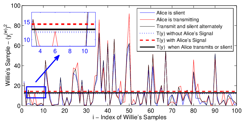
Next we provide an experimentally-supported analysis of this methods. Fig. 3 illustrates an example of sequences of 100 Willie’s samples $[y_{1}^{(w)}]^{2},...,[y_{n}^{(w)}]^{2}$ in the case that Alice is silent, transmitting, or transmitting and silent alternately. Willie then computes $T(\mathbf{y})=\frac{1}{n}\sum^{n}_{k=1}[y_{k}^{(w)}]^{2}$ . Clearly, when Alice alternates transmission with silence, Willie’s sample value $T(\textbf{y})$ will decrease and quite near the value when Alice is silent. For this reason, the alternation of Alice can increase Willie’s uncertainty. The transmitted signals resemble white noise, and are sufficiently weak in this way.

With the same simulation settings of Fig. 3, we evaluate Willie’s sample values $T(\textbf{y})$ by varying the transmit power $P_{t}$ . As displayed in Fig. 4, the value $T(\textbf{y})$ changing with $P_{t}$ is displayed in three cases, i.e., Alice is transmitting, silent, as well as transmitting and silent alternately. We find that when Alice employs the alternation method, Willie’s sample values decrease, approximating to the case Alice is silent. Further, the results indicate that higher transmit power cannot lead to stronger capability for Willie to distinguish Alice’s transmission behavior. With the transmit power increases, Willie’s sample values $T(\textbf{y})$ increase. However, the aggregated interference increases as well, resulting in the gap of sample values between Alice’s transmission and silence does not increase. Consequently, this is consistent with the result of Theorem 1, which indicates that increasing the transmit power $P_{t}$ does not increase the risk of being detected by Willie.

Further, as Theorm 1 states, one of critical factors affecting covert communication is the parameter $d_{a,w}$ , the distance between Alice and Willie, which should satisfies $d_{a,w}=\omega(n^{\delta/4})$ to ensure communication covertly. Fig. 5 illustrates Willie’s sample values $T(\textbf{y})$ by varying the distance $d_{a,w}$ . As the results show, when Alice is silent, Willie’s sample values $T(\textbf{y})$ barely change since Willie only experiences the noise and aggregated interference. When Alice is transmitting, persistence or alteration, Willie’s sample values increase with decreasing the distance $d_{a,w}$ . When $d_{a,w}\leq 1$ , Willie’s sample values become relatively stable since we employ the bounded path loss law $l(x)=\min\{1,r^{-\alpha}\}$ .

For the following analysis, we evaluate the effect of the number of samples $n$ on the distance between Alice and Willie $d_{a,w}$ . We start by comparing Willie’s sample values by varying $n$ to show the difference in performance. The results in Fig. 6 shows $T(\textbf{y})$ with respect to the distance $d_{a,w}$ when $n=1000$ and $n=3000$ . As can be seen, although the curves of the average $T(\textbf{y})$ do not change, the discreteness of $T(\textbf{y})$ decreases with increasing the number of samples $n$ . As to Willie, to detect Alice’s transmission attempts, he should distinguish the three lines in the picture with relatively low probability of error. The only way to decrease the probability of error is increasing the number of samples. By choosing a larger value for $n$ , Willie’s uncertainty on noise and interference decreases, hence he can stay far away from Alice to detect her transmission attempt. As illustrated in Fig. 6(a), Willie cannot distinguish Alice’s transmission from silence when he stays at a distance of more than 1 meter to Alice. However, when Willie increases the number of samples, he can distinguish Alice’s behavior far away. As depicted in Fig. 6(b), Willie can detect Alice’s transmission at the distance between 1 and 1.5 meters with low probability of error. Overall, this experimental result agrees with the theoretical derivation and conclusion of Theorem 1, i.e., given the value $n$ , the distance between Alice and Willie should be larger than a bound to ensure the covertness, and the bound of $d_{a,w}$ increases with the increasing of $n$ , $d_{a,w}=\omega(n^{\delta/4})$ .

IV-D Traffic Shaping and Willie’s Sample Dilemma

A practical way for Alice to avoid being detected is leveraging traffic shaping [34] as her transmission scheduling such that packet transmission and silence are alternative in time slots. As depicted in Fig. 7, Alice divides a chunk of data into packets and transmit each packet in the odd slots. Traffic shaping may be implemented with for example the leaky bucket or token bucket algorithm. Traffic shaping used in this occasion is not to optimize or increase usable bandwidth, it is used to uniform the transmission of Alice. Although it may increases the transmission latency, Willie’s uncertainty also increases.

Willie’s Sample Dilemma: As discussed earlier, when Willie increases the number of samples, he can distinguish Alice’s behavior at greater distance. According to Equ. (39) and (42), a larger quantity of samples of Willie will lead to smaller variance of $T(\mathbf{y})|\mathbf{H_{0}}$ and $T(\mathbf{y})|\mathbf{H_{1}}$ . Hence Willie’s uncertainty will decrease with the increase of samples. However, to confuse Willie, Alice can divide the slots sufficiently small and insert her message in the slots uniformly. When Willie gathers samples, more samples he collects, more signals of Alice will be included in his samples. If Willie employs a radiometer as his detector, it is difficult for him to distinguish between hypotheses $\mathbf{H_{0}}$ and $\mathbf{H_{1}}$ . Therefore, how to determine the number of samples is a dilemma that Willie has to be confronted with. As to Alice, her better policy is alternating transmission and idle periods, that is, “telling a short story in a long period, speaking for a short time and taking a rest for a while.”

IV-E Time Interval and Slow Start

Because Willie employs a radiometer as his detector, to obtain a relatively accurate estimation of noise, he first gathers a large quantity of samples to determine his detection threshold. After that, he leverages the threshold to determine whether Alice is transmitting or not in an interval by comparing the threshold with the samples in this new interval.

At first, Alice has to determine the proper time intervals of transmission and idle states. Fig. 8(a) illustrates Alice’s transmission scheduling with different slot assignments, Fig. 8(b) depicts Willie’s sampling value by varying the distance between Alice and Willie for different transmission scheduling schemes. We can find that, if Alice’s transmission slot is wider than the idle slot, Willie’s sampling value may greater than his detection threshold with high probability, resulting in the exposure of Alice’s transmission behavior. When Alice’s transmission slot is shorter than her idle slot, Willie’s sampling value may less than his detection threshold, and Willie can deduce that Alice is in her idle state at this time. Therefore, the optimal slot assignment method is to set the length of the transmission slot and idle slot in the same length, i.e., $p=0.5$ . As shown in Fig. 8(b) when $p=0.5$ , the sampling values change around the threshold value, making it difficult for Willie to determine whether Alice is transmitting or not. Besides, the slot should be as short as possible to make Willie’s samples contain more Alice’s signal.

Slow Start and Slow Stop: If Alice is transmitting while Willie is sampling the channel to determine the interference level and his detection threshold, Willie’s samples will contain Alice’s signals. If Willie later employs this threshold to test Alice’s behavior, he will not be able to ascertain Alice’s transmission behavior. However, if Alice is not transmitting while Willie begins his sampling, Willie’s detection threshold will be lower than that when Alice is transmitting. Therefore Willie will have higher probability to find the transmission attempt when Alice transmits later. Lower transmission probability implies weaker transmitted signal. As depicted in Fig. 8(b), Willie’s sampling value with $p=0.1$ is much lower than the sampling value with $p=0.5$ but a little higher than that when Alice is idle. Therefore, to decrease the probability of being detected, Alice should transmit with lower transmission probability $p=0.1$ from the very beginning, and slowly increasing until $p=0.5$ . Conversely, Alice should slowly stop her transmission in case of being detection when she has no more messages to transmit further.

In the scene that network traffic is sparse or not evenly spread in the whole network, the aggregated interference may be too weak to cover the transmission attempts or unevenly distributed. In the case of sparse traffic, potential transmitters should resort to recruiting “friendly” nodes to generate artificial noise, such as the methods used in [23]. In the case of uneven traffic distribution, the better way is using some effective methods, such as routing protocols, to homogenize the network traffic.

In most practical scenarios, to detect the transmission attempt of Alice, Willie should approach Alice as close as possible, and ensure that there is no other node located closer to Willie than Alice. Otherwise, Willie cannot determine which one is the actual transmitter. But in a wireless network, some wireless nodes are probably placed on towers, trees, or buildings, Willie cannot get close enough as he wishes. Furthermore, wireless networks are diverse and complicated. If Willie is not definitely sure that there is no other transmitter in his vicinity, he cannot ascertain that Alice is transmitting. However, in a mobile wireless network, some mobile nodes may move into the detection region of Willie, and increase the uncertainty of Willie. Therefore mobile can improve the performance of covert communication to some extend.

V Conclusions

In this paper, we have studied the covert wireless communication with the consideration of interference uncertainty. Prior studies on covert communication only considered the background noise uncertainty, or introduced collaborative jammers producing artificial noise to help Alice in hiding the communication. By introducing interference measurement uncertainty, we find that uncertainty in noise and interference experienced by Willie is beneficial to Alice, and she can achieve undetectable communication with better performance. If Alice want to hide communications with interference in noisy wireless networks, she can reliably and covertly transmit $\mathcal{O}(\log_{2}\sqrt{n})$ bits to Bob in $n$ channel uses. Although the covert rate is lower than the square root law and the friendly jamming scheme, its spatial throughput is higher as $n\rightarrow\infty$ . From the network perspective, the communications are hidden in the noisy wireless networks. It is difficult for Willie to ascertain whether a certain user is transmitting or not, and what he sees is merely a shadow wireless network.

References

[1] B. A. Bash, D. Goeckel, D. Towsley, and S. Guha, “Hiding information in noise: Fundamental limits of covert wireless communication,” IEEE Communications Magazine, vol. 52, no. 12, pp. 26–31, December 2015.
[2] J. Hu, C. Lin, and X. Li, “Relationship privacy leakage in network traffics,” in 25th International Conference on Computer Communication and Networks, ICCCN, August 2016, pp. 1–9.
[3] P. Kamat, Y. Zhang, W. Trappe, and C. Ozturk, “Enhancing source-location privacy in sensor network routing,” in Proceedings of the 25th IEEE International Conference on Distributed Computing Systems, ICSCS’05, Columbus, Ohio, USA, June 2005, pp. 599–608.
[4] B. Bash, D. Goeckel, and D. Towsley, “Limits of reliable communication with low probability of detection on awgn channels,” IEEE Journal on Selected Areas in Communications, vol. 31, no. 9, pp. 1921–1930, September 2013.
[5] B. A. Bash, D. Goeckel, and D. Towsley, “Covert communication gains from adversary¡¯s ignorance of transmission time,” IEEE Transactions on Wireless Communications, vol. 15, no. 12, pp. 8394–8405, 2016.
[6] S. Lee, R. J. Baxley, M. A. Weitnauer, and B. Walkenhorst, “Achieving undetectable communication,” IEEE Journal of Selected Topics in Signal Processing, vol. 9, no. 7, pp. 1195–1205, October 2015.
[7] R. Tandra and A. Sahai, “Snr walls for signal detection,” IEEE Journal of Selected Topics in Signal Processing, vol. 2, no. 1, pp. 4–17, February 2008.
[8] B. He, S. Yan, X. Zhou, and V. K. N. Lau, “On covert communication with noise uncertainty,” IEEE Communications Letters, vol. 21, no. 4, pp. 941–944, April 2017.
[9] L. Wang, G. W. Wornell, and L. Zheng, “Fundamental limits of communication with low probability of detection,” IEEE Transactions on Information Theory, vol. 62, no. 6, pp. 3493–3503, June 2016.
[10] M. R. Bloch, “Covert communication over noisy channels: A resolvability perspective,” IEEE Transactions on Information Theory, vol. 62, no. 5, pp. 2334–2354, May 2016.
[11] R. Soltani, D. Goeckel, D. Towsley, and A. Houmansadr, “Covert communications on renewal packet channels,” in 54th Annual Allerton Conference on Communication, Control, and Computing (Allerton). Monticello, IL, USA: IEEE, September 2016, pp. 548–555.
[12] P. Gupta and P. R. Kumar, “The capacity of wireless networks,” IEEE Transactions on Information Theory, vol. 46, no. 2, pp. 388–404, March 2000.
[13] S. Weber and J. G. Andrews, “Transmission capacity of wireless networks,” Foundations and Trends®in Networking, vol. 5, no. 2-3, pp. 109–281, 2010.
[14] M. Bloch and J. Barros, Physical-Layer Security: From Information Theory to Security Engineering. Cambridge University Press, September 2011.
[15] W. Trappe, “The challenges facing physical layer security,” IEEE Communications Magazine, vol. 53, no. 6, pp. 16–20, June 2015.
[16] D. Goeckel, S. Vasudevan, D. Towsley, S. Adams, Z. Ding, and K. Leung, “Artificial noise generation from cooperative relays for everlasting secrecy in two-hop wireless networks,” IEEE Journal on Selected Areas in Communications, vol. 29, no. 10, pp. 2067–2076, December 2011.
[17] S. Goel and R. Negi, “Guaranteeing secrecy using artificial noise,” IEEE Transactions on Wireless Communications, vol. 7, no. 6, pp. 2180–2189, June 2008.
[18] Y. Allouche, Y. Cassuto, A. Efrat, M. Segal, E. M. A. G. Grebla, J. S. B. Mitchell, and S. Sankararaman, “Secure communication through jammers jointly optimized in geography and time,” in ACM MobiHoc’15, Hangzhou, China, June 2015, pp. 227–236.
[19] S. Gollakota, H. Hassanieh, B. Ransford, D. Katabi, and K. Fu, “They can hear your heartbeats: Non-invasive security for implantable medical devices,” in ACM SIGCOMM, New York, NY, USA, 2011, pp. 2–13.
[20] T. V. Sobers, B. A. Bash, D. Goeckel, S. Guha, and D. Towsley, “Covert communication with the help of an uninformed jammer achieves positive rate,” in 49th Asilomar Conference on Signals, Systems and Computers, Pacific Grove, CA, USA, November 2015, pp. 625–629.
[21] T. V. Sobers, B. A. Bash, S. Guha, D. Towsley, and D. Goeckel, “Covert communication in the presence of an uninformed jammer,” IEEE Transactions on Wireless Communications, vol. 16, no. 9, pp. 6193–6206, 2017.
[22] R. Soltani, B. Bashy, D. Goeckel, S. Guhaz, and D. Towsley, “Covert single-hop communication in a wireless network with distributed artificial noise generation,” in Fifty-second Annual Allerton Conference, Allerton House, UIUC, Illinois, USA, October 2014, pp. 1078–1085.
[23] R. Soltani, D. Goeckel, D. Towsley, B. A. Bash, and S. Guha, “Covert wireless communication with artificial noise generation,” CoRR, vol. abs/1709.07096, 2017. [Online]. Available: http://arxiv.org/abs/1709.07096
[24] S. P. Weber, J. G. Andrews, X. Yang, and G. de Veciana, “Transmission capacity of wireless ad hoc networks with successive interference cancellation,” IEEE Transactions on Information Theory, vol. 53, no. 8, pp. 2799–2814, August 2007.
[25] J. Fridrich, Steganography in Digital Media: Principles, Algorithms, and Applications, 1st ed. Cambridge Univ. Press, 2009.
[26] M. K. Simon, J. K. Omura, R. A. Scholtz, and B. K. Levitt, Spread Spectrum Communications Handbook, revised edition ed. McGraw-Hill, 1994.
[27] S. Zander, G. Armitage, and P. Branch, “A survey of covert channels and countermeasures in computer network protocols,” IEEE Communications Surveys Tutorials, vol. 9, no. 3, pp. 44–57, Third 2007.
[28] S. Cabuk, C. E. Brodley, and C. Shields, “Ip covert timing channels: design and detection,” in Proceedings of 11th ACM conf. Computer and communication security, CCS’04. New York, USA: ACM, September 2004, pp. 178–187.
[29] M. Haenggi, Stochastic Geometry for Wireless Networks, 1st ed. New York, NY, USA: Cambridge University Press, 2012.
[30] S. Weber, J. G. Andrews, and N. Jindal, “An overview of the transmission capacity of wireless networks,” IEEE Transactions on Communications, vol. 58, no. 12, pp. 3593–3604, December 2010.
[31] ——, “The effect of fading, channel inversion, and threshold scheduling on ad hoc networks,” IEEE Transactions on Information Theory, vol. 53, no. 11, pp. 4127–4149, 2007.
[32] M. Haenggi and R. K. Ganti, “Interference in large wireless networks,” Foundations and Trends®in Networking, vol. 3, no. 2, pp. 127–248, 2008.
[33] M. Haenggi, “On distances in uniformly random networks,” IEEE Transactions on Information Theory, vol. 51, no. 10, pp. 3584–3586, 2005.
[34] S. Blake, D. Black, M. Carlson, E. Davies, Z. Wang, and W. Weiss, “An architecture for differentiated services - section 2.3.3.3 - internet standard definition of “shaper”,” Internet Requests for Comments, RFC Editor, RFC 2475, July 1998.

The Sound and the Fury: Hiding Communications in Noisy Wireless Networks with Interference Uncertainty

Abstract

Index Terms:

I Introduction

II Problem Formulation and System Model

II-A Motivating Scenario

II-B Channel Model

II-C Network Model

II-D Hypothesis Testing

III Covert Communication With Interference Uncertainty in Noisy Wireless Networks

III-A Achievability

III-A1 Covertness

III-A2 Reliability

III-B Converse

IV Discussions

IV-A Spatial Throughput

IV-B Interference Uncertainty

IV-C Practical Method and Experimental Results

IV-D Traffic Shaping and Willie’s Sample Dilemma

IV-E Time Interval and Slow Start

V Conclusions

References

The Sound and the Fury:
Hiding Communications in Noisy Wireless Networks with Interference Uncertainty